Models of Production Lines as Quasi-Birth-Death Processes
MEHMET MURAT FADILOGLU, Bilkent University
SENCER YERALAN, Rigel Corporation
Industrial Engineering Department Bilkent University
Bilkent, Ankara 06533 Turkey
Abstract: The aim of this work is to illustrate the suitability of Quasi-Birth-Death Processes (QBDs) for stochastic modeling of production lines. With this end in mind, first, an introduction to QBDs is made, so that the reader who may not be acquainted with this aspect of stochastic modeling may be introduced to the basics of the topic. Then, a formal definition of QBD is given and the QBDs are contrasted with the traditional birth-death processes. Later, examples of QBD models pertaining to production lines are presented. The rational of this exposition is to show how QBDs present themselves within the context of production lines and to show the kind of work that needs to be performed to fully specify the corresponding QBD. By compiling the aforementioned models, the strength of QBDs in modeling production lines is demonstrated.
1 Introduction to Quasi-Birth-Death Processes:
The study of Quasi-Birth-Death Processes (QBDs) goes back to R. V. Evans [1] and to V. Wallace [2]. In fact, Wallace coined the term “Quasi-Birth-Death Process”. Yet, the most comprehensive study is by Neuts [3]. Since all the following research refers to Neuts for the basics of the field, it is appropriate to give his definition:
A QBD is a Markov process on the state space E ={(i,j),i≥0,1≤ j≤m},
with the infinitesimal generator
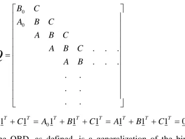
Q
, given by = . . . . . . . . . . . . 0 0 ~ B A C B A C B A C B A C B
Q
(1) where B01T +C1T = A01T +B1T +C1T = A1T +B1T +C1T =0.The QBD, as defined, is a generalization of the birth-death process. Birth-death processes are stochastic processes of Markov type where each state can be associated with an element of a counting set, which effectively means that the states can be ordered in a linear fashion. Once the correct ordering is established, transitions should occur only to neighboring states: that means given that the process is in state n, it can have a transition only to state n+1 or state n-1. And the transition times are exponentially distributed which allows their classification under the general category of Markov processes. As with any Markov process, a state transition diagram (Figure 1) can be used to represent it.
1 2 3 . . . N N+1 . . .
.
Figure 1 Basic birth-death process model
In the case of the QBD, instead of one state corresponding to an element of the counting set, there is a group of states corresponding to it. Thus, from a given group of states, the process can have transitions to the group of states corresponding to the previous element of the counting set or to the group of states corresponding to the next element of the counting set. This kind of Markov process yields a state transition diagram of the form shown in Figure 2.
1 2 3 . . . N N+1 . . .
Figure 2 Representation of a QBD ( The dashed lines represent a collection of transitions originating from a state in one group and terminate in a state in another group.)
According to Neuts’ definition, a QBD is defined by a generator matrix that has a block nested tridiagonal structure in which the same blocks are repeated infinitely many times except for the initial states. For this to occur, one would need to have the same number of states corresponding to each counting set element. Moreover, the same kind of transitions with the same transition rates should be present in between these states. Thus all literature that adopts the definition of Neuts really relates to state-homogeneous quasi-birth-death processes.
Within the framework defined for QBDs, it is most appropriate to define the state space as the Kroenicker product of two sets, one of which is the counting set. Thus, the other set is used to distinguish all possible things that can happen at a given counting set level. The same things should be possible at all counting set levels and the way the process goes from one of them to another should be independent of the level.
The QBDs that Neuts investigates differ in one way from the ones that are the subject of this study. The counting set is infinite, in other words the counting set is the set of natural numbers for Neuts’ case. A finite counting set is used here, since no production system is likely to have infinite buffers. This means that instead of having only one boundary there are two boundaries for these QBDs.
A formal definition for the kind of QBD used here is:
A QBD is a Markov process on the state space , with the transition rate matrix –or the infinitesimal generator-- } 1 , 0 ), , {(i j i M j n E = ≤ ≤ ≤ ≤ R , given by
= M B A C B A C B A C B A C B R . . . . . . . . . 0 (2) where B01T +C1T = A1T +B1T +C1T = A1T +BM1T =0.
This will be the definition of QBD in this paper. An interesting observation is that the structure of equation (2) has been already shown to be of great use in the modeling of production lines in the seminal work by Yeralan and Muth [4]. Three works following this lead, Tan [5], Yeralan and Tan [6], Fadiloglu and Yeralan [7] exploit this structure in finding the steady-state probabilities by applying a matrix-polynomial solution procedure. The computational effort in the procedure is independent of the cardinality of the counting set of the QBD. Thus, the QBD models have the additional advantage of being amenable to an efficient solution procedure. Furthermore, the spectral theory based on the procedure carries the prospect of furthering the understanding of the behavior modeled systems manifest.
2 QBD Models for Production Lines
Although the QBD platform is quite general and can be used for many stochastic models that pertain to different areas, in this paper, examples of QBD models pertaining to production lines are examined. A similar effort can be conducted for other areas, which give rise to QBDs, but the scope of the present research is limited to the models of production lines, which have been studied extensively by many scholars due to the importance of the subject [8].
In this section production line models are presented in a natural progression. First, basic models, and then, more complex models that mimic further behavior of real production systems are introduced. The submatrices that define the QBD for each model will be specified. Once these are produced, the models are ready for application of the matrix polynomial procedure.
Model 1: Exponential Server with Limited Buffer
A graphical representation for the model is given in Figure 3. This is most probably the first model to be encountered in any queuing theory book, the quintessential M/M/1 model. Here, the only deviation from this basic model is that the buffer–or the queue–has a limited size, M. Usually this is named M/M/1/M, with the last M representing the size of the queue. In this model, parts arrive to the server as a Poisson process with a mean rate of λ , and they are serviced with exponential service times with mean µ.
λ
M
µ
Figure 3 Exponential server with limited buffer and its relevant parameters
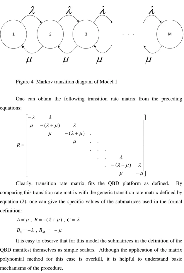
One can obtain the Markov chain diagram shown in Figure 4 using this description for the model. As one can observe from the diagram, this model is actually a simple birth-death process. But since QBD is a generalization of birth-death process this model still qualifies for the name QBD. Actually it forms one of the simplest QBDs possible. One can easily write the steady-state equations for this model by looking at the diagram:
0 ) 1 ( ) 0 ( + = −λP µP 1 1 0 ) 1 ( ) 1 ( ) ( ) ( + + + + − = ≤ ≤ − − λ µ P i µP i λP i for i M 0 ) 1 ( ) ( + − = −µP M λP M
1 2 3
. . .
Mλ
λ
λ
λ
µ
µ
µ
µ
Figure 4 Markov transition diagram of Model 1
One can obtain the following transition rate matrix from the preceding equations: − + − + − + − − = µ µ λ µ λ λ µ µ λ µ λ µ λ µ λ λ ) ( . . . . . . . . . ) ( ) ( R
Clearly, transition rate matrix fits the QBD platform as defined. By comparing this transition rate matrix with the generic transition rate matrix defined by equation (2), one can give the specific values of the submatrices used in the formal definition: λ µ λ µ =− + = = B C A , ( ) , µ λ = − − = BM B0 ,
It is easy to observe that for this model the submatrices in the definition of the QBD manifest themselves as simple scalars. Although the application of the matrix polynomial method for this case is overkill, it is helpful to understand basic mechanisms of the procedure.
Model 2: Exponential Server with Breakdown and Repair, Limited Buffer
A graphical representation for the model is given in Figure 5. This model builds on Model 1 by incorporating breakdown and repair capability. If the server is
operating, it breaks down with a time to breakdown distribution that is exponential with parameter α . Once the breakdown occurs, the repair starts. The time to the end of repair is also exponentially distributed with parameter β. During the breakdown, the part that was being processed at the time breakdown occurred is not processed. Processing starts on the same part after the repair.
λ
M
µ
On/Off
)
/
(
α
β
Figure 5 Exponential server with breakdown and repair and its relevant parameters.
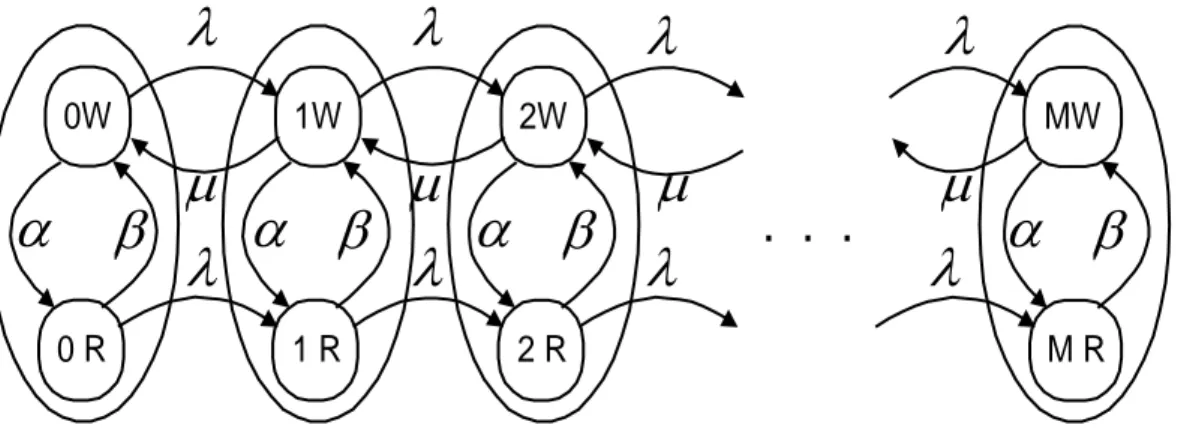
For the described process the Markov transition diagram is given in Figure 6. It is clear that the state space is the Kroenicker product of the counting set with a set of two elements {W,R}. W corresponds to the states for which the server is working and R corresponds to the states for which the station is broken and the repair is taking place. 0W 0 R
α β
1W 1 Rα β
2W 2 Rα β
MW M Rα β
. . .
λ
λ
λ
λ
λ
λ
λ
λ
µ
µ
µ
µ
The steady-state equations for the process are 0 ) , 1 ( ) , 0 ( ) , 0 ( ) ( + + + = − α λ P W βP R µP W 0 ) , 0 ( ) , 0 ( ) ( + + = − β λ P R αP W 1 1 0 ) , 1 ( ) , 1 ( ) , ( ) , ( ) ( + + + + − + + = ≤ ≤ − − α λ µ P i W βP i R λP i W µP i W for i M 1 1 0 ) , 1 ( ) , ( ) , ( ) ( + + + − = ≤ ≤ − − λ µ P i R αP i W λP i R for i M 0 ) , 1 ( ) , ( ) , ( ) ( + + + − = − α µ P M W βP M R λP M W 0 ) , 1 ( ) , ( ) , ( + + − = −βP M R αP M W λP M R
One can obtain the following transition rate matrix from the preceding equations: − + − + − + + − + − + + − + − + − = β β α µ α µ λ λ β β λ α µ λ α λ β β α µ λ α µ λ λ β β λ α λ α 0 0 ) ( 0 0 ) ( . . 0 ) ( . . . . . . . . . . . . . . . . . . . . ) ( 0 0 . . ) ( 0 0 ) ( 0 ) ( R
Clearly, this transition rate matrix conforms to the definition of a QBD as stated. The dimension of the submatrices is 2x2 and the submatrices can be easily extracted: = + − + + − = = λ λ λ β β α µ λ α µ 0 0 , ) ( ) ( , 0 0 0 C B A − + − = + − + − = β β α µ α λ β β α λ α ( ) , ) ( ) ( 0 BM B
Model 3: Server With Erlang-2 Service Times, Limited Buffer
The only difference between this model, depicted in Figure 7, and Model 1 is the statistical distribution of the service times. In the M/M/1 model the distribution is exponential, whereas here it is Erlang which is the sum of two exponential distributions with the same rate. In order to accommodate for this non-exponential
distribution, one needs to incorporate an additional state for each counting level. When this idea is applied, one gets the Markov transition diagram shown in Figure 8.
λ
M
Erlang
(
2
,
µ
)
Figure 7 Server with Erlang-2 service times, limited buffer and its relevant parameters.
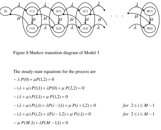
The state space is the Kroenicker product of the counting set and the set {1,2}, which keeps track of the Erlang stage in the processing of parts. Here, only one state corresponds to the element 0 of the counting set. Consequently, this element cannot be incorporated in the QBD and has to be handled separately. The QBD starts from element 1. This has to be taken into account while applying the matrix polynomial solution procedure. (0) (1,1) (1,2) (2,1) (2,2) (3,1) (3,2) (M,1) (M,2)
. . .
λ
λ
λ
λ
λ
λ
λ
λ
λ
µ
µ
µ
µ
µ
µ
µ
µ
µ
Figure 8 Markov transition diagram of Model 3
The steady-state equations for the process are 0 ) 2 , 1 ( ) 0 ( + = −λP µP 0 ) 2 , 2 ( ) 0 ( ) 1 , 1 ( ) ( + + + = − λ µ P λP µP 0 ) 2 , 1 ( ) 1 , 1 ( ) ( + + = − λ µ P µP 0 ) 2 , 1 ( ) 1 , 1 ( ) 1 , ( ) ( + + − + + = − λ µ P i λP i µP i for 2≤i≤M −1 0 ) 1 , ( ) 2 , 1 ( ) 2 , ( ) ( + + − + = − λ µ P i λP i µP i for 2≤i≤M −1 0 ) 1 , 1 ( ) 1 , ( + − = −µP M λP M
0 ) 1 , ( ) 2 , 1 ( ) 2 , ( + − + = −µP M λP M µP M
After substituting the value of obtained from the first equation into the second equation, one can obtain the following transition rate matrix from the preceding equations: ) 0 ( P − − + − + − + − + − + − + − = µ µ µ µ λ µ λ λ µ µ λ µ λ µ µ µ λ λ λ β µ λ µ µ λ 0 0 0 0 0 ) ( 0 . . 0 ) ( . . . . . . . . . . . . . . . . . . . . ) ( 0 0 . . ) ( 0 0 0 ) ( 0 ) ( R
Clearly, this transition rate matrix conforms to the definition of a QBD as stated. The dimension of the submatrices is 2x2 and the submatrices can be easily extracted: = + − + − = = λ λ µ λ µ µ λ µ 0 0 , ) ( 0 ) ( , 0 0 0 C B A − − = + − + − = µ µ µ µ λ µ µ µ λ 0 , ) ( ) ( 1 BM B
Model 4: Server With Erlang-2 Service Times, Breakdown and Repair, Limited Buffer
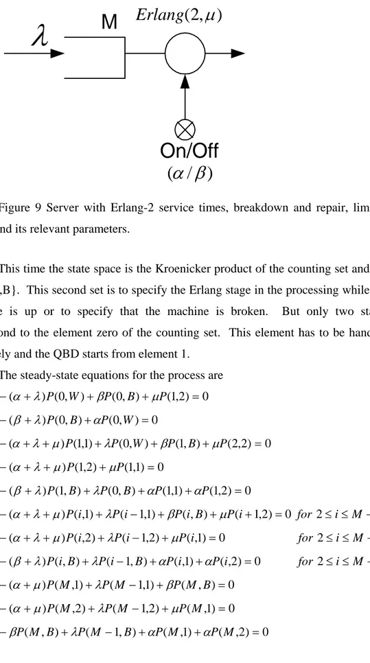
This model, depicted in Figure 9, combines the characteristics of Model 2 and Model 3. There is breakdown and repair mechanism just as in Model 2. However, the production times are distributed with Erlang-2 distribution as the case is in Model 3. To accommodate for these, one needs three states corresponding to each counting set level. The Markov transition diagram for the process is given in Figure 10.
λ
M
On/Off
)
/
(
α
β
)
,
2
(
µ
Erlang
Figure 9 Server with Erlang-2 service times, breakdown and repair, limited buffer and its relevant parameters.
This time the state space is the Kroenicker product of the counting set and the set {1,2,B}. This second set is to specify the Erlang stage in the processing while the machine is up or to specify that the machine is broken. But only two states correspond to the element zero of the counting set. This element has to be handled separately and the QBD starts from element 1.
The steady-state equations for the process are 0 ) 2 , 1 ( ) , 0 ( ) , 0 ( ) ( + + + = − α λ P W βP B µP 0 ) , 0 ( ) , 0 ( ) ( + + = − β λ P B αP W 0 ) 2 , 2 ( ) , 1 ( ) , 0 ( ) 1 , 1 ( ) ( + + + + + = − α λ µ P λP W βP B µP 0 ) 1 , 1 ( ) 2 , 1 ( ) ( + + + = − α λ µ P µP 0 ) 2 , 1 ( ) 1 , 1 ( ) , 0 ( ) , 1 ( ) ( + + + + = − β λ P B λP B αP αP 0 ) 2 , 1 ( ) , ( ) 1 , 1 ( ) 1 , ( ) ( + + + − + + + = − α λ µ P i λP i βP i B µP i for 2≤i≤M −1 0 ) 1 , ( ) 2 , 1 ( ) 2 , ( ) ( + + + − + = − α λ µ P i λP i µP i for 2≤i≤M −1 0 ) 2 , ( ) 1 , ( ) , 1 ( ) , ( ) ( + + − + + = − β λ P i B λP i B αP i αP i for 2≤i≤M −1 0 ) , ( ) 1 , 1 ( ) 1 , ( ) ( + + − + = − α µ P M λP M βP M B 0 ) 1 , ( ) 2 , 1 ( ) 2 , ( ) ( + + − + = − α µ P M λP M µP M 0 ) 2 , ( ) 1 , ( ) , 1 ( ) , ( + − + + = −βP M B λP M B αP M αP M
β (0,W) (0,B) (1,1) (1,2) (1,B) (1,1) (1,1) (1,2) (1,B) (1,1) (1,1) (1,2) (1,B) (1,1) (1,1) (1,2) (1,B) (1,1) . . . . . . α α α α α α α α β ββ β λ λ λ λ λ λ λ λ λ λ λ λ λ λ µ µ µ µ µ µ µ µ µ
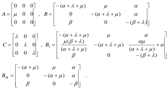
After substituting the values of and obtained from the first two equations into the third and fifth equations, one can obtain the transition rate matrix which is of the form given in Equation (2). The submatrices should be defined as ) , 0 ( W P P(0,B) + − + + − + + − = = ) ( 0 ) ( 0 ) ( , 0 0 0 0 0 0 0 0 λ β β α µ λ α α µ µ λ α µ B A + − + + + + + − + + ++ + − = = ) ( 0 ) ( ) ( ) ( ) ( ) ( , 0 0 0 0 0 0 1 λ β β α µ λ α αµ µ λ α µ λ α λ β µα λ µ µ α λ λ λ B C − + − + − = β β α µ α α µ µ α 0 ) ( 0 ) ( M B .
Model 5: Two Exponential Servers with One Intermediate Limited Buffer
In this model shown in Figure 11, two exponential servers are present and the buffer is placed between the servers. The typical two-server model in the literature assumes an infinite source for the server, which is the stochastic equivalent of Model 1. The input is a Poisson process. One can assume that there is a second buffer at the input of the system. But the size of this buffer would be limited to one. In following models, the difficulties faced when a generic sized second buffer is incorporated in the models are illustrated. The Markov transition diagram for the process is given in Figure 12.
λ
µ
1
M
µ
2
Figure 11 Two exponential servers with one intermediate limited buffer and its relevant parameters.
The state space is the Kroenicker product of the counting set and the set {0,1}. The counting set relates to the buffer level as usual. The set {0,1} can be considered as the level of an imaginary first buffer whose size is one; in other words it tells whether there is a part being processed in server one.
(0,0) (0,1) (0,0) (0,1) (0,0) (0,1) (0,0) (0,1) . . . . . .
λ
µ
1λ
µ
1λ
µ
1µ
1λ
µ
2µ
2µ
2µ
2µ
2µ
2µ
2µ
2Figure 12 Markov transition diagram of Model 5
The steady-state equations for the process are 0 ) 0 , 1 ( ) 0 , 0 ( + 2 = −λP µ P 0 ) 1 , 1 ( ) 0 , 0 ( ) 1 , 0 ( 2 1 + + = −µ P λP µ P 0 ) 0 , 1 ( ) 1 , 1 ( ) 0 , ( ) ( + 2 + 1 − + 2 + = − λ µ P i µ P i µ P i for 1≤i≤M −1 0 ) 1 , 1 ( ) 0 , ( ) 1 , ( ) ( 1+ 2 + + 2 + = − µ µ P i λP i µ P i for 1≤i≤M −1 0 ) 1 , 1 ( ) 0 , ( ) ( + 2 + 1 − = − λ µ P M µ P M 0 ) 0 , ( ) 1 , ( 2 + = −µ P M λP M
This process conforms to the definition of a QBD as stated. Thus all one has to do for formally defining the QBD is to state the relevant submatrices whose sizes are 2x2: = + − + − = = 0 0 0 , ) ( 0 ) ( , 0 0 1 2 1 2 2 2 µ µ µ λ µ λ µ µ C B A − + − = − − = 2 2 1 0 0 ) ( , 0 µ λ µ λ µ λ λ M B B
Model 6: Two Exponential Servers With One Intermediate Limited Buffer, Breakdown and Repair
This model depicted in Figure 13 is an extension of Model 4. The breakdown and repair mechanisms are added to two basic servers of Model 4. Both servers become non-operational when a breakdown occurs at the server, up to the time that the repair ends. Thus, the production process is hindered by these occurrences. These breakdowns and repairs occur independently in both servers. The modeling of this system requires a large number of states for each intermediate buffer level as illustrated in the Markov transition diagram of the process in Figure 14.
λ
M
On/Off
On/Off
)
/
(
α
1β
1 1µ
µ
2
)
/
(
α
2β
2Figure 13 Two exponential servers with one intermediate limited buffer, breakdown and repair and its relevant parameters
The state space for this model is the Kroenicker product of four sets: the counting set C–which appears in all the QBDs–modeling the intermediate buffer level, the set S1 = {W,R} modeling the repair status of the first server, the set L1 =
{0,1} modeling number of parts in server one, and the set S2 = {W,R} modeling the
(0 ,W,0,W) (0 ,R ,0,W) (0 ,W,0,R ) (0 ,R ,0,B) (0 ,W,1,W) (0 ,W,1,R ) (0 ,R ,1,W) (0 ,R ,1,R ) (0 ,W,0,W) (0 ,R ,0,W) (0 ,W,0,R ) (0 ,R ,0,B) (0 ,W,1,W) (0 ,W,1,R ) (0 ,R ,1,W) (0 ,R ,1,R ) (0 ,W,0,W) (0 ,R ,0,W) (0 ,W,0,R ) (0 ,R ,0,B) (0 ,W,1,W) (0 ,W,1,R ) (0 ,R ,1,W) (0 ,R ,1,R ) (0 ,W,0,W) (0 ,R ,0,W) (0 ,W,0,R) (0 ,R ,0,B) (0 ,W,1,W) (0 ,W,1,R) (0 ,R ,1,W) (0 ,R ,1,R ) . . . . . . . . . . . . λ λ λ λ α1 α1 α1 α1 α1 α1 α1 α1 α1 α1 α1 α1 α1 α1 α1 α1 β1 β1 β1 β1 β1 β1 β1 β1 β1 β1 β1 β1 β1 β1 β1 β1 α2 α2 α2 α2 α2 α2 α2 α2 α2 α2 α2 α2 α2 α2 α2 α2 λ λ λ λ λ λ λ λ λ λ β2 β2 β2 β 2 β2 β2 β2 β2 β2 β2 β2 β2 β2 β2 β2 β2 µ2 µ2 µ2 µ2 µ2 µ2 µ2 µ2 µ2 µ2 µ2 µ2 µ2 µ2 µ2 µ2 µ1 µ1 µ1 µ1 µ1 µ1 µ1 µ1 λ λ
The steady-state equations for the process are 0 ) , 0 , , 1 ( ) , 0 , , 0 ( ) , 0 , , 0 ( ) , 0 , , 0 ( ) ( + 1+ 2 + 1 + 2 + 2 = − λ α α P W W βP W R β P R W µ P W W 0 ) , 0 , , 1 ( ) , 0 , , 0 ( ) , 0 , , 0 ( ) , 0 , , 0 ( ) ( + 2 + 2 + 1 + 2 + 2 = − λ α β P W R α P W W β P R R µ P W R 0 ) , 1 , , 1 ( ) , 1 , , 0 ( ) , 1 , , 0 ( ) , 0 , , 0 ( ) , 1 , , 0 ( ) ( 2 2 1 1 2 1 = + + + + + + − W W P W R P R W P W W P W W P µ β β λ µ α α 0 ) , 1 , , 1 ( ) , 1 , , 0 ( ) , 1 , , 0 ( ) , 0 , , 0 ( ) , 1 , , 0 ( ) ( 2 2 1 1 2 = + + + + + − R W P R R P W W P R W P R W P µ β α λ β α 0 ) , 0 , , 0 ( ) , 0 , , 0 ( ) , 0 , , 0 ( ) ( + 1+ 2 + 2 + 1 = − λ α β P R W α P W W β P R R 0 ) , 0 , , 0 ( ) , 0 , , 0 ( ) , 0 , , 0 ( ) ( + 1+ 2 + 1 + 2 = − λ β β P R R α P R W α P W R 0 ) , 1 , , 0 ( ) , 1 , , 0 ( ) , 0 , , 0 ( ) , 1 , , 0 ( ) ( 1+ 2+ 1 + + 2 + 1 = − α β µ P R W λP R W α P W W β P R R 0 ) , 1 , , 0 ( ) , 1 , , 0 ( ) , 0 , , 0 ( ) , 1 , , 0 ( ) ( 1+ 2 + + 1 + 2 = − β β P R R λP R R α P R W α P W R 0 ) , 1 , , 1 ( ) , 0 , , 1 ( ) , 0 , , ( ) , 0 , , ( ) , 0 , , ( ) ( 1 2 2 1 2 2 1 = − + + + + + + + + − W W i P W W i P W R i P R W i P W W i P µ µ β β µ α α λ 1 1≤i≤M − for 0 ) , 0 , , 1 ( ) , 0 , , ( ) , 0 , , ( ) , 0 , , ( ) ( 2 2 1 2 2 2 = + + + + + + + − R W i P R R i P W W i P R W i P µ β α µ β α λ 1 1≤i≤M − for 0 ) , 1 , , 1 ( ) , 1 , , ( ) , 1 , , ( ) , 0 , , ( ) , 1 , , ( ) ( 2 2 1 2 1 2 1 = + + + + + + + + − W W i P W R i P R W i P W W i P W W i P µ β β λ µ µ α α 1 1≤i≤M − for 0 ) , 1 , , 1 ( ) , 1 , , ( ) , 1 , , ( ) , 0 , , ( ) , 1 , , ( ) ( 2 2 1 2 1 2 = + + + + + + + − R W i P R R i P W W i P R W i P R W i P µ β α λ µ β α for 1≤i≤M −1 0 ) , 1 , , 1 ( ) , 0 , , ( ) , 0 , , ( ) , 0 , , ( ) ( 1 1 2 2 1 = − + + + + + − W R i P R R i P W W i P W R i P µ β α β α λ for 1≤i≤M −1 0 ) , 0 , , ( ) , 0 , , ( ) , 0 , , ( ) ( + 1+ 2 + 1 + 2 = − λ β β P i R R α Pi R W α P iW R for 1≤i≤M −1 0 ) , 1 , , ( ) , 1 , , ( ) , 0 , , ( ) , 1 , , ( ) ( 1 2 1 2 1 = + + + + + − R R i P W W i P W R i P W R i P β α λ µ β α 1 1≤i≤M − for 0 ) , 1 , , ( ) , 1 , , ( ) , 0 , , ( ) , 1 , , ( ) ( 2 1 2 1 = + + + + − R W i P W R i P R R i P R R i P α α λ β β for 1≤i≤M −1 0 ) , 1 , , 1 ( ) , 0 , , ( ) , 0 , , ( ) , 0 , , ( ) ( 1 2 1 2 2 1 = − + + + + + + − W W M P W R M P R W M P W W M P µ β β µ α α λ 0 ) , 0 , , ( ) , 0 , , ( ) , 0 , , ( ) ( + 2 + 2 + 2 + 1 + 2 = − λ α β µ P M W R α P M W W β P M R R 0 ) , 1 , , ( ) , 1 , , ( ) , 0 , , ( ) , 1 , , ( ) ( 2 1 2 2 1 = + + + + + − W R M P R W M P W W M P W W M P β β λ µ α α
0 ) , 1 , , ( ) , 1 , , ( ) , 0 , , ( ) , 1 , , ( ) ( 2 1 2 1 2 = + + + + + − R R M P W W M P R W M P R W M P β α λ µ β α 0 ) , 1 , , 1 ( ) , 0 , , ( ) , 0 , , ( ) , 0 , , ( ) ( 1 1 2 2 1 = − + + + + + − W R M P R R M P W W M P W R M P µ β α β α λ 0 ) , 0 , , ( ) , 0 , , ( ) , 0 , , ( ) ( + 1+ 2 + 1 + 2 = − λ β β P M R R α P M R W α P M W R 0 ) , 1 , , ( ) , 1 , , ( ) , 0 , , ( ) , 1 , , ( ) ( 1+ 2 + + 2 + 1 = − α β P M R W λP M R W α P M W W βP M R R 0 ) , 1 , , ( ) , 1 , , ( ) , 0 , , ( ) , 1 , , ( ) ( 1+ 2 + + 1 + 2 = − β β P M R R λP M R R α P M R W α P M W R
This process conforms to the definition of a QBD as defined. Thus, all one has to do for formally defining the QBD is to state the relevant submatrices whose sizes are 8x8: = 0 0 0 0 0 0 0 0 0 0 0 0 0 0 0 0 0 0 0 0 0 0 0 0 0 0 0 0 0 0 0 0 0 0 0 0 0 0 0 0 0 0 0 0 0 0 0 0 0 0 0 0 0 0 0 0 0 0 0 0 2 2 2 2 µ µ µ µ A , = 0 0 0 0 0 0 0 0 0 0 0 0 0 0 0 0 0 0 0 0 0 0 0 0 0 0 0 0 0 0 0 0 0 0 0 0 0 0 0 0 0 0 0 0 0 0 0 0 0 0 0 0 0 0 0 0 0 0 0 0 0 0 1 1 µ µ C + − + + − + + − + + − + + − + + + − + + + − + + + − = ) ( 0 0 0 0 0 ) ( 0 0 0 0 0 0 ) ( 0 0 0 0 ) ( 0 0 0 0 0 0 ) ( 0 0 0 0 0 ) ( 0 0 0 0 0 0 ) ( 0 0 0 0 ) ( 2 1 1 2 1 1 2 1 2 2 1 1 2 1 2 1 2 2 2 1 2 1 2 1 2 1 2 1 2 2 1 2 1 2 1 2 2 1 β β β β α µ β α β λ β β λ β β λ α β α λ β α µ β α β α α µ µ α α α λ µ β α λ β α λ α µ α α λ B + − + + − + + − + + − + − + + − + + − + + − = ) ( 0 0 0 0 0 ) ( 0 0 0 0 0 0 ) ( 0 0 0 0 ) ( 0 0 0 0 0 0 ) ( 0 0 0 0 0 ) ( 0 0 0 0 0 0 ) ( 0 0 0 0 ) ( 2 1 1 2 1 1 2 1 1 2 2 1 1 2 1 2 1 2 2 1 2 1 2 1 1 2 1 2 1 2 1 2 1 2 1 0 β β β β α µ β α β λ β β λ β β λ α β α λ β α β α β α α µ α α α λ β α λ β α λ α α α λ B
+ − + − + + − + + − + + − + + − + + + − + + + − = ) ( 0 0 0 0 0 ) ( 0 0 0 0 0 0 ) ( 0 0 0 0 ) ( 0 0 0 0 0 0 ) ( 0 0 0 0 0 ) ( 0 0 0 0 0 0 ) ( 0 0 0 0 ) ( 2 1 1 2 1 2 1 2 2 1 1 2 1 2 1 2 2 2 1 2 1 2 1 2 2 1 2 2 1 2 1 2 1 2 2 1 β β β β α β α β λ β β λ β β λ α β α λ β α µ β α β α α µ α α α λ µ β α λ β α λ α µ α α λ M B
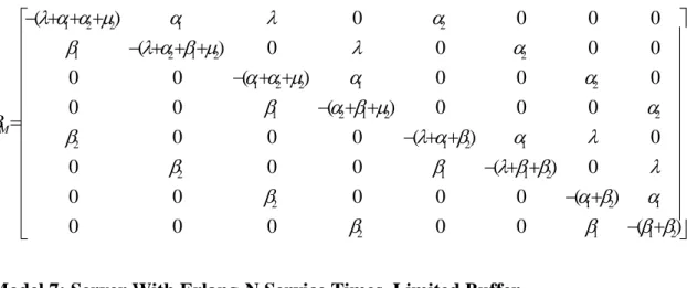
Model 7: Server With Erlang-N Service Times, Limited Buffer
In Model 3, the case when the server has Erlang-2 service times is studied. In this model depicted in Figure 15 this model is extended to Erlang-N service times. The number of states in this model increases both with M and N. Yet the matrix polynomial solution procedure does not depend on the size of the counting space which is the buffer size here. But the larger the Erlang parameter is, the larger the submatrices are. Thereby, the computational effort increases with the parameter N. The Markov transition diagram of the process is given below:
λ
M
Erlang
(
N
,
µ
)
Figure 15 Server with Erlang-N service times, limited buffer and its relevant parameters.
The state space for this model is the Kroenicker product of two sets: the counting set C that corresponds to the buffer level and the Erlang stage set S. The Erlang stage set itself, is also a counting set. Thus one can have two different matrix representations for the QBD: one using the buffer level as the counting set of the QBD and one using the Erlang stage set. But since there is a transition from the Erlang stage N to Erlang stage 1, the choice of Erlang stage set would not yield a QBD as defined.
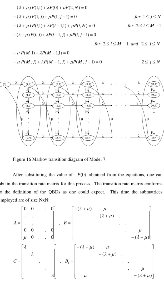
The steady-state equations for the process are 0 ) , 1 ( ) 0 ( + = −λP µP N
0 ) , 2 ( ) 0 ( ) 1 , 1 ( ) ( + + + = − λ µ P λP µP N 0 ) 1 , 1 ( ) , 1 ( ) ( + + − = − λ µ P j µP j for 1≤ j≤N 0 ) , ( ) 1 , 1 ( ) 1 , ( ) ( + + − + = − λ µ P i λP i µP i N for 2≤i≤M −1 0 ) 1 , ( ) , 1 ( ) , ( ) ( + + − + − = − λ µ P i j λPi j µPi j for 2≤i ≤M −1 and 2≤ j≤N 0 ) 1 , 1 ( ) 1 , ( + − = −µP M λP M 0 ) 1 , ( ) , 1 ( ) , ( + − + − = −µP M j λP M j µP M j 2≤ j≤N (0) (1,1) (1,2) (1,3) (1,N) . . . (2,1) (2,2) (2,3) (2,N) . . . (3,1) (3,2) (3,3) (3,N) . . . (M,1) (M,2) (M,3) (M,N) . . . . . . . . . . . . . . . λ λ λ λ λ λ λ λ λ λ λ λ λ λ λ λ λ µ µ µ µ µ µ µ µ µ µ µ µ µ µ µ µ µ µ µ µ
Figure 16 Markov transition diagram of Model 7
After substituting the value of obtained from the equations, one can obtain the transition rate matrix for this process. The transition rate matrix conforms to the definition of the QBDs as one could expect. This time the submatrices employed are of size NxN:
) 0 ( P + − + − + − = = ) ( . . . . ) ( ) ( , 0 . . 0 0 . . 0 0 . . . . . . 0 . . 0 0 µ λ µ µ λ µ µ λ µ B A = λ λ λ . . C , + − + − + − = ) ( . . . . ) ( ) ( 1 µ λ µ µ µ λ µ µ λ B
− − − = µ µ µ µ µ . . . . M B
If one wanted to use Erlang stage set as the counting set, he would not get the a QDP in the strict sense of the word, but something quite close to it. And the matrix polynomial solution procedure for obtaining the steady-state probabilities would still be applicable since the deviation from the QDP definition would only occur in the boundary equations. This is due to the fact that the matrix polynomial solution procedure is based on the structure of the inner equations. It does not preclude a deviation from the definition in boundary equations.
The transition rate matrix obtained with such a choice would be of the form
= M M B A X C B A C B A B A C B A X C B R 0 0 . . . . . . (3)
This one is a generalization of the transition rate matrix given in equation (2). One can observe that two impurities are allowed at the corners of the matrix.
Once this transition rate matrix is defined, one can write the transition rate matrix of the process with the Erlang stage used as the counting set within this platform. Indeed to define the submatrices in the (3) would suffice:
− + − + − + − = µ λ µ λ λ µ λ λ µ λ ) ( . . . . ) ( ) ( B , B1 =B
− − − − = µ µ µ µ µ µ µ . . . . M B , , = µ µ µ . . C A=0 = 0 0 . . . . 0 0 0 1 µ µ µ µ X , XM =0
Model 8: Two Exponential Servers with Two Limited Buffers
This model depicted in Figure 17 is an extension on the Model 5. In Model 5, the first server does not have a buffer for the arrivals. Thereby, those arrivals that occur while the server is occupied are lost. In this model, those arrivals are stored in a buffer whose size is M1. This model is quite important because it is a tandem queue,
which happens to form the basic building block of many models for modern production systems. Yet, a theoretically sound methodology has not developed to tackle the stochastic analysis of this queue class up to this point.
λ
µ
1M
22
µ
1
M
Figure 17 Two exponential servers with two limited buffers and their relevant parameters
To perform stochastic analysis of this model, one can generate a Markov chain using a large state-space to incorporate the second queue. Though this is a valid
option, it is not viable for many real models since the computational effort increases with the size of the state space. Moreover it is not conducive to obtain parametric results from which one can obtain an idea about the behavior of such systems.
Within the platform of matrix polynomial solution procedure, one can solve QBDs with an effort independent of the size of the counting set. Yet, for the tandem queues one does not have only one counting set but many of them. For this model with two tandem queues, there are two counting sets, each corresponding to the buffer levels of the two servers.
(0,0) (0,1) (0,2) (0,M2) (1,0) (1,1) (1,2) (2,0) (2,1) (2,2) (1,M2) (2,M2) (M1,0) (M1,1) (M1,0) (M1,M2)
λ
λ
λ
λ
λ
λ
λ
λ
λ
λ
λ
λ
λ
λ
λ
λ
1µ
µ
1µ
1µ
1 1µ
µ
1µ
1µ
1 1µ
µ
1µ
1 1µ
µ
1µ
1µ
1 2µ
µ
2µ
2µ
2 2µ
µ
2µ
2µ
2 2µ
µ
2µ
2µ
2 2µ
µ
2µ
2µ
2. . .
. . .
. . .
. . .
.
.
.
.
.
.
.
.
.
.
.
.
Figure 18 Markov transition diagram of Model 8
Since the matrix polynomial methodology only allows the exploitation of the structure for a single counting set, one cannot make use of the second counting set. One point to consider is the choice of the principal counting set of the QBD. The logical strategy for this is to choose the one with higher cardinality. Then, the computational effort that relates to the solution decreases.
The Markov transition diagram pertaining to the model is given in Figure 18. One can clearly observe by examining the diagram that the state space is the Kroenicker product of two counting sets: the first buffer level set C1 = {1,2,3, …, M1}
element of C1 and the second index of C2. One also observes that there are M1.M2
states in the model.
The steady-state equations for the process are
0 ) 1 , 0 ( ) 0 , 0 ( + 2 = −λP µ P 0 ) 1 , ( ) 0 , 1 ( ) 0 , ( ) ( + 1 + − + 2 = − λ µ P i λP i µ P i for 1≤i≤M1−1 0 ) 1 , ( ) 0 , 1 ( ) 0 , ( 1 1 2 1 1 + − + = −µ P M λP M µ P M 0 ) 1 , 0 ( ) 1 , 1 ( ) , 0 ( ) ( + 2 + 1 − + 2 + = − λ µ P j µ P j µ P j for 1≤ j≤M2 −1 0 ) 1 , 1 ( ) , 0 ( ) ( + 2 2 + 1 2 − = − λ µ P M µ P M 0 ) 1 , ( ) 1 , 1 ( ) , 1 ( ) , ( ) ( + 1 + 2 + − + 1 + − + 2 + = − λ µ µ P i j λP i j µ P i j µ P i j for 1≤i≤M1 −1 1≤ j ≤M2 −1 0 ) 1 , 1 ( ) , 1 ( ) , ( ) ( + 2 2 + − 2 + 1 + 2 − = − λ µ P i M λP i M µ P i M for 1≤ j ≤M2 −1 0 ) 1 , ( ) , 1 ( ) , ( ) ( 1+ 2 1 + 1− + 2 1 + = − µ µ P M j λP M j µ P M j for 1≤ j≤M2 −1 0 ) , 1 ( ) , ( 1 2 1 2 2 + − = −µ P M M λP M M
Lucidly, this process conforms to the definition of the QBD. Moreover, one has two choices for the counting set. If the set C1 is elected as the counting set, the
submatrices that define the QBD are of the dimension M2xM2. These relevant
submatrices are = 0 . . . . 0 0 0 1 1 1 µ µ µ A , C = λ λ λ . . + − + + − + + − + + − + − = ) ( ) ( . . . . ) ( ) ( ) ( 2 2 2 1 2 2 1 2 2 1 2 1 µ λ µ µ µ λ µ µ µ λ µ µ µ λ µ µ λ B
+ − + − + − + − − = ) ( ) ( . . . . ) ( ) ( 2 2 2 2 2 2 2 2 0 µ λ µ µ λ µ µ λ µ µ λ µ λ B − + − + − + − − = ) ( ) ( . . . . ) ( ) ( 2 2 2 1 2 2 1 2 2 1 2 1 1 µ µ µ µ µ µ µ µ µ µ µ µ M B
If the set C2 is elected as the counting set, the submatrices that define the QBD
are of the dimension M1xM1. These relevant submatrices are
= 2 2 2 . . µ µ µ A , = 0 0 . . . . 0 0 2 2 2 µ µ µ C + − + + − + + − + + − + − = ) ( ) ( . . . . ) ( ) ( ) ( 2 1 2 1 2 1 2 1 2 µ µ λ µ µ λ λ µ µ λ λ µ µ λ λ µ λ B − + − + − + − − = 1 1 1 1 0 ) ( . . . . ) ( ) ( µ λ µ λ λ µ λ λ µ λ λ λ B
− + − + − + − + − = 2 2 2 2 2 ) ( . . . . ) ( ) ( ) ( 2 µ λ µ λ λ µ λ λ µ λ λ µ λ M B
The interesting phenomena that one should observe is that the block tridiagonal structure that is the insignia of the QBD is also exhibited in each of the submatrices that has been presented. Indeed, it is possible to show that this phenomenon generalizes for tandem queues having more than two buffers. For each buffer, there would be another level of trigonal structure embedded in the blocks belonging to the previous level.
One can relate this phenomenon to fractals. The same kind of macro-structure appears in the elements of the whole. As one gets to examine these submatrices, the same structure exhibits itself. And the amount that this self-similarness occurs is the number of stations–and thereby the number of buffers–in the tandem queue.
Although no methodology to fully exploit this marvelous structure -- in order to obtain the nullspace of the transition rate matrix—exists at this point, it can still be quite useful in generating the transition rate matrix for a given process in an efficient fashion.
4 Conclusion
In this paper, the suitability of QBD platform in the stochastic modeling of the production lines is illustrated. First, an introduction to QBDs is made. Then, 8 examples of how production lines with different characteristics can be modeled as QBDs, are presented. It is obvious that it would not be difficult to augment the number of these examples by using the same principles. The more complicated the nature of the modeled system is, more states corresponding to each element of the counting space would be needed.
By using the methodology described in the papers by Fadiloglu and Yeralan [7], and Yeralan and Tan [6] one can find the steady-state probabilities for these models irrespective of the counting set’s cardinality. In the models, the counting set
always corresponds to a buffer of choice. Yet when more than one buffer exists, one comes up with a structure we can call Multi-Dimensional Quasi-Birth-Death Process. This process is still a QBD, thus amenable to the same solution methodologies. Yet, there is some additional structure in these processes as has been illustrated in Model 8. The exploitation of this structure would be an important addition to this line of research.
REFERENCES
[1] Evans, R.V. (1967), “Geometric Distribution in Some Two-dimensional Queuing Systems,” Operations Research, Vol. 15, pp. 830-846.
[2] Wallace, V. (1969), “The Solution of Quasi Birth and Death Processes Arising from Multiple Access Computer Systems,” Ph.D. Thesis, Systems Engineering Laboratory, University of Michigan, Ann Arbor.
[3] Neuts, M.F. (1981), Matrix-Geometric Solutions in Stochastic Models: An Algorithmic Approach, Johns Hopkins Press, Baltimore.
[4] Yeralan, S. and Muth, E.J. (1987), “A General Model of a Production Line with Intermediate Buffer and Station Breakdown,” IIE Transactions, Vol. 19, No. 2, pp. 130-139.
[5] Tan, B. (1994), “A Decomposition Method for Multistation Production Systems”, Ph.D. Dissertation, Industrial and Systems Engineering, University of Florida, Gainesville.
[6] Yeralan, S. and Tan, B. (1997), “Analysis of Multistation Production Systems with Limited Buffer Capacity Part 1: The Subsystem Model,” Mathematical and Computer Modelling, Vol. 25, No. 7, pp.109-122.
[7] Fadiloglu, M. M., and Yeralan, S. (1998), “A General Theory on Spectral Properties of State-Homogeneous Quasi-Birth-Death Processes”, to appear in European Journal of Operational Research
[8] Dallery, Y., and Gershwin, S.B. (1992), “Manufacturing Flow Line Systems: A Review of Models and Analytical Results,” Queuing Systems, Vol. 12, No. 3, pp. 3-94.