Analysis of cross-correlations between financial markets after the 2008 crisis

Analysis of cross-correlations between financial markets

after the 2008 crisis

✩,✩✩

A. Sensoy

a,b,∗

, S. Yuksel

a

, M. Erturk

a

a_{Borsa Istanbul, Research Department, Resitpasa Mahallesi, Tuncay Artun Caddesi, Emirgan, Istanbul, 34467, Turkey} b_{Bilkent University, Department of Mathematics, Ankara, 06800, Turkey}

h i g h l i g h t s

• We use RMT to analyze the cross-correlations between worldwide stock markets. • We find that the majority of the cross-correlation coefficients arise from randomness.

• We analyze the connection structure of markets before and after the crisis using network theory. • Key financial markets are revealed.

a r t i c l e i n f o

Article history:

Received 30 December 2012 Received in revised form 23 April 2013 Available online 25 June 2013 Keywords:

Cross-correlations Random matrix theory Complex systems Minimal spanning tree Centrality measures

a b s t r a c t

We analyze the cross-correlation matrix C of the index returns of the main financial mar-kets after the 2008 crisis using methods of random matrix theory. We test the eigenvalues of C for universal properties of random matrices and find that the majority of the cross-correlation coefficients arise from randomness. We show that the eigenvector of the largest deviating eigenvalue of C represents a global market itself. We reveal that high volatility of financial markets is observed at the same times with high correlations between them which lowers the risk diversification potential even if one constructs a widely internationally di-versified portfolio of stocks. We identify and compare the connection and cluster structure of markets before and after the crisis using minimal spanning and ultrametric hierarchical trees. We find that after the crisis, the co-movement degree of the markets increases. We also highlight the key financial markets of pre and post crisis using main centrality mea-sures and analyze the changes. We repeat the study using rank correlation and compare the differences. Further implications are discussed.

© 2013 Elsevier B.V. All rights reserved. 1. Introduction

The global financial system is composed of a large variety of markets that are positioned in different geographic locations and in which a broad range of financial products are traded. Despite the diversity of markets, index movements often

respond to the same economic announcements or market news [1–3] which implies that financial time series can display

similar characteristics and be correlated. Since the work of Markowitz [4], correlations of financial time series are constantly

✩ _{The views expressed in this work are those of the authors and do not necessarily reflect those of the Borsa Istanbul or its members.}

✩✩_{An earlier version of this paper was presented at the ‘‘Asian Quantitative Finance Conference’’ organized by the National University of Singapore, January}

9–11, 2013 and the ‘‘Conference on Mathematics in Finance’’ organized by the Bank of England and the Institute of Mathematics and its Applications, in Edinburgh, April 8–9, 2013. We thank the conference participants for insightful suggestions.

∗_{Corresponding author at: Borsa Istanbul, Research Department, Resitpasa Mahallesi, Tuncay Artun Caddesi, Emirgan, Istanbul, 34467, Turkey. Tel.: +90}

5326959943; fax: +90 2122982189.

E-mail addresses:ahmets@fen.bilkent.edu.tr,ahmet.sensoy@borsaistanbul.com(A. Sensoy). 0378-4371/$ – see front matter©2013 Elsevier B.V. All rights reserved.

a subject of extensive studies both at the theoretical and practical levels. It is important not only for understanding the collective behavior of a complex system but also for asset allocation and estimating the risk of a portfolio.

In particular since the recent 2008 financial crisis, which originated in the US and then spread to almost all markets in the world, many economists have been studying the correlation structure between financial markets and the transmission of volatility from one to another. One of the major difficulties in these studies are the complicated unknown underlying interactions of the financial markets. Besides correlations between markets need not be just pairwise but may rather involve

clusters of markets and relationship between any two pair may change in time [5].

In earlier times, physicists experienced similar problems. The problem became popular by Wigner’s work in the 1950s for application in nuclear physics, in the study of statistical behavior of neutron resonances and other complex systems of

interactions [6]. He tried to understand the energy levels of complex nuclei, when model calculations failed to explain

exper-imental data. To overcome this problem, he assumed that the interactions between the constituents comprising the nucleus

are so complex that they can be modeled as random [5]. Based on this assumption, he derived the statistical properties of

very large symmetric matrices with i.i.d. entries and the results were in remarkable agreement with experimental data.

More recently random matrix theory (RMT) has been applied to analyze the financial time series [5,7–37]. In particular,

correlation matrices are computed for the empirical data and quantities associated with these matrices are compared to those of random matrices. The extent to which properties of the correlation matrices deviate from random matrix

predications clarifies the status of the information derived from the computation of covariances [12]. The literature focuses

on the correlations between individual stocks in a market; however, in this study we will analyze the cross-correlations between 87 main financial markets in the world by tools of RMT.

The rest of the paper is organized as follows; in Section2, we give a brief description of the methodology. Section3

describes the data and contains several results of our analysis; in particular Sections3.1,3.2and3.4present the eigenvalue

and eigenvector analysis of the correlation matrix with discussion of the relation between volatility and correlation of

financial markets. In Section3.6, we construct a correlation based market network and compare the structure before and

after the 2008 financial crisis by tools of graph theory. In Section4, we use an alternative approach to the construction

of the correlation matrix, present the related results and discuss possible further studies. Finally, Section5contains some

concluding remarks.

2. Methodology

Let Pi

(

t

)

be the index of the stock market i

=

1

,

2

, . . . ,

N at time t and t

=

0

,

1

, . . . ,

T . The logarithmic index return of

the ith market index over a time interval1t is given by

Ri

(

t

,

1t

) ≡

ln Pi

(

t

+

1t

) −

ln Pi

(

t

).

(1)

We consider the normalized returns

ri

(

t

) ≡

Ri

− ⟨

Ri

⟩

σ

i (2) where

σ

i

≡



⟨

R2_i

⟩ − ⟨

Ri

⟩

2is the standard deviation of Riand

⟨· · ·⟩

is the time average over the considered period. Then the equal time cross-correlation matrix C is the matrix with elements

cij

≡ ⟨

rirj

⟩

.

(3)

In matrix notation, the interaction matrix C can be written as

C

=

1

TRR

t ₍₄₎

where R is an N

×

T matrix with entries rim

≡

ri

(

m1t

)

with i

=

1

,

2

, . . . ,

N; m

=

1

, . . . ,

T and Rtdenotes the transpose of

R.

We will compare the properties of the interaction matrix C with those of a random cross-correlation matrix.

Let xi

(

t

)

; i

=

1

,

2

, . . . ,

N where xi

(

t

)

are independent, identically distributed random variables. We define the N

×

T

matrix A by elements ait

≡

xi

(

t

)

. The matrix W defined as

W

=

1

TAA

t ₍₅₎

is called a Wishart matrix [38–40]. Let each xi

(

t

)

be normally distributed and rescaled to have zero mean and constant unit

standard deviation. Under the restriction of N

→ ∞

, T

→ ∞

with Q

≡

T

/

N

>

1 is fixed, the probability density function

ρ

rm

(λ)

of eigenvalues

λ

of the matrix W is [39,40]

ρ

rm

(λ) =

Q 2

π

√

(λ

max

−

λ)(λ − λ

min

)

λ

(6)

ρ

Wnn

(

s

) =

2 exp

−

4s

2 ₍₈₎

where s

=

α

_i+1

−

α

i.

The distribution of next-nearest neighbor eigenvalue spacing of W is given by [41,42]:

ρ

Wnnn

(

s

) =

218 36

π

3s 4_exp



−

64 9

π

s 2



(9) where s

=

(α

_i+2

−

α

i

)/

2.

The number variance



2

is defined as the variance of the number of unfolded eigenvalues in the intervals of length l,

around each

α

i[41,42],



2

(

l

) = ⟨[

n

(α,

l

) −

l

]

2

⟩

_α (10)

where n

(α,

l

)

is the number of unfolded eigenvalues in the interval

[

α −

l

/

2

, α +

l

/

2

]

and

⟨· · ·⟩

_αdenotes an average over

all

α

. For large values of l, the number variance for W behaves like



2

_∼

ln l and if the eigenvalues are uncorrelated then



2

_∼

l [41,42].

Let

v

kbe the eigenvector corresponding to the eigenvalue

λ

k. We denote the jth component of

v

kas

v

k,j. By construction

we have



N

j=1

[

v

k,j

]

2

=

1. If we normalize the eigenvectors (

v

k

→

v

′k) such that



N j=1

[

v

′

k,j

]

2

=

N then the components of

each normalized eigenvector

v

′

khave a Gaussian distribution with mean zero and unit variance [10],

ρ(v

′

_{) =}

_√

1 2

π

exp



−

v

′2 2



.

(11)

A useful quantity in characterizing the eigenvectors is the so-called Inverse Participation Ratio (IPR) [11]. For the

eigen-vector

v

k, it is defined as IPRk

≡

N



j=1

[

v

_k,j

]

4

.

(12)

For our purposes it is sufficient to know that the reciprocal of the IPRk(called participation ratio) quantifies the number of

significant components of the eigenvector

v

k. In RMT, the expectation of IPRkis 3

/

N since the kurtosis for the distribution

of the eigenvector component is 3.

3. Data and the results

We analyze daily closing values of 87 main benchmark indexes in the world between 01/01/2009 and 31/07/2012 (data are obtained from Bloomberg). To reflect the market dynamics better, index values are not converted to a single currency. Markets in some countries do not operate on Fridays; in that case Saturdays’ values are considered as Fridays’. If a market

is closed on a business day, we carry over the last value. The list of indexes is in theAppendix.

3.1. Eigenvalue analysis

We take1t

=

1 day and compute the 87

×

87 cross-correlation matrix C. We have N

=

87 and T

=

933 giving Q

≈

10

.

73, with theoretical lower and upper limits

λ

min

≈

0

.

48 and

λ

max

≈

1

.

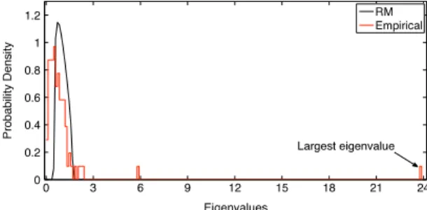
71 for the eigenvalues of C. First, eigenvalues of C

are compared with the theoretical distribution

ρ

rm

(λ)

(seeFig. 1).

One immediate thing to note is that the largest eigenvalue of C is

≈

23

.

8 which is 14 times larger than the theoretical

upper limit and stands out from all others. Also a first view suggests the presence of a well-defined bulk of eigenvalues.

Although

≈

52% of the eigenvalues fall into the theoretical interval,

≈

93% of the eigenvalues are smaller than

λ

max.1

1 The high percentage of eigenvalues belowλminmay be attributed to the fact that many of the less liquid markets behave independently relative to the rest of the others [12], and also theoretical results are also valid in the infinite limit; hence there is always a small probability of finding eigenvalues above

Fig. 1. Empirical vs. theoretical eigenvalue distribution.

a

_b

Fig. 2. Simulation (finite size (a)–fat tails (b)) vs. theoretical eigenvalue distribution.

a

_b

Fig. 3. Nearest and next-nearest neighbor spacing distribution of eigenvalues.

Since the theoretical distribution is valid strictly for N

→ ∞

and T

→ ∞

, we must test that the deviations for the largest

few eigenvalues are not finite size effects [11]. First, we construct N

=

87 mutually uncorrelated time series generated to

have (a) standard normal distribution (as in theory), and (b) identical power-law tails (as in empirical examples [43]) each

having length T

=

933. Then we compare eigenvalue densities of their cross-correlation matrices with the theoretical

dis-tribution (seeFig. 2). We find good agreement with the theory suggesting that the deviations of the few largest eigenvalues

from RMT inFig. 1are not caused by finite size effects or the fact that returns are fat tailed.2

We apply further RMT tests to strength our claim. The first independent test is the comparison of the distribution of

empirical nearest neighbor eigenvalue spacing

ρ

nn

(

s

)

with

ρ

Wnn

(

s

)

(seeFig. 3). The agreement suggests that the positions of

two adjacent empirical unfolded eigenvalues at the distance s are correlated similar to the eigenvalues of W.

The next test is the comparison of the distribution of empirical next-nearest neighbor eigenvalue spacing

ρ

nnn

(

s

)

with

ρ

Wnnn

(

s

)

. We demonstrate this correspondence inFig. 3which shows a nice agreement between empirical data and the

theory.

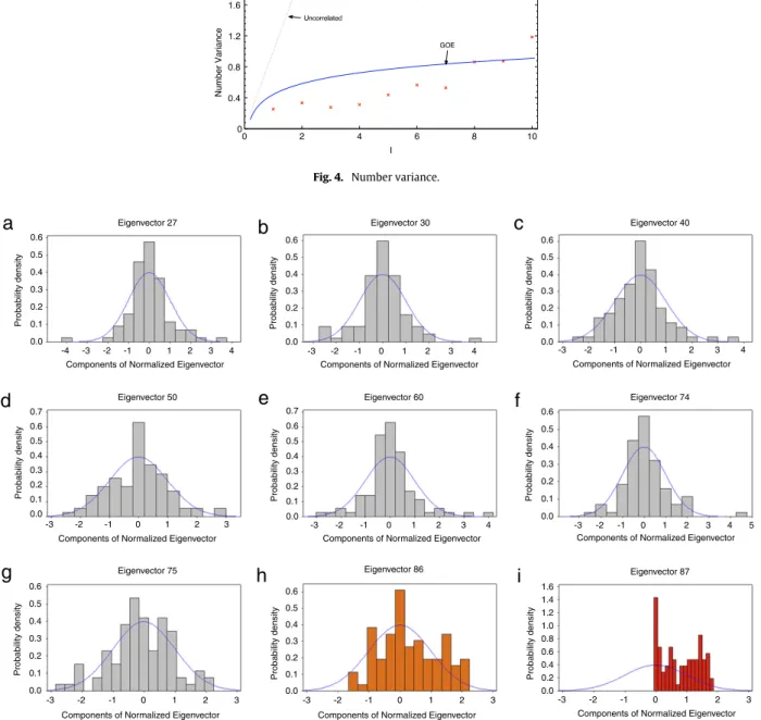
To test for long-range two point eigenvalue correlations, we consider the number variance. It is clear that the number

variance of empirical data agrees well with the theory (seeFig. 4).

It can be concluded that the bulk of the eigenvalue statistics of the empirical cross-correlation matrix C are consistent with those of the real symmetric random matrix W and the deviations from the RMT contain genuine information about the correlations in the system.

Fig. 4. Number variance. 0.6 0.5 0.4 0.3 0.2 0.1 0.0 Probability density Probability density Probability density Eigenvector 27 Eigenvector 50 Eigenvector 75 Eigenvector 60 Eigenvector 86 Eigenvector 74 Eigenvector 87 Eigenvector 30 Eigenvector 40 -4 -3 -2 -1 0 1 2 3 4

Components of Normalized Eigenvector Components of Normalized Eigenvector 0.6 0.5 0.4 0.3 0.2 0.1 0.0 Probability density 0.6 0.5 0.4 0.3 0.2 0.1 0.0 Probability density -3 -2 -1 0 1 2 3 4

Components of Normalized Eigenvector Components of Normalized Eigenvector

Components of Normalized Eigenvector -3 -2 -1 0 1 2 3

Components of Normalized Eigenvector 4

Components of Normalized Eigenvector 0.6 0.7 0.5 0.4 0.3 0.2 0.1 0.0 Probability density Probability density -3 -2 -1 0 1 2 3

Components of Normalized Eigenvector

0.6 0.7 0.5 0.4 0.3 0.2 0.1 0.0 -3 -2 -1 0 1 2 3 4 0.6 0.5 0.4 0.3 0.2 0.1 0.0 -3 -2 -1 0 1 2 3 4 5 -3 -2 -1 0 1 2 3 0.6 0.5 0.4 0.3 0.2 0.1 0.0

Probability density Probability density

-3 -2 -1 0 1 2 3

Components of Normalized Eigenvector -3 -2 -1 0 1 2 3 0.6 0.5 0.4 0.3 0.2 0.1 0.0 1.6 1.4 1.2 1.0 0.8 0.6 0.4 0.2 0.0

a

_b

c

d

e

f

g

_h

_i

Fig. 5. Density of components of the normalized eigenvectors.

3.2. Eigenvector analysis

The deviations of eigenvalue statistics from the RMT results suggest that these deviations should also be displayed in the

statistics of corresponding eigenvector components [43]. First, we choose some of the normalized eigenvectors and display

their component distribution inFig. 5which shows that the probability density of eigenvector components corresponding

to eigenvalues in the bulk agrees well with the RMT. However, the component distribution of

λ

i

> λ

maxshows significant

deviation from the theory. In particular

ρ(v

′

87

)

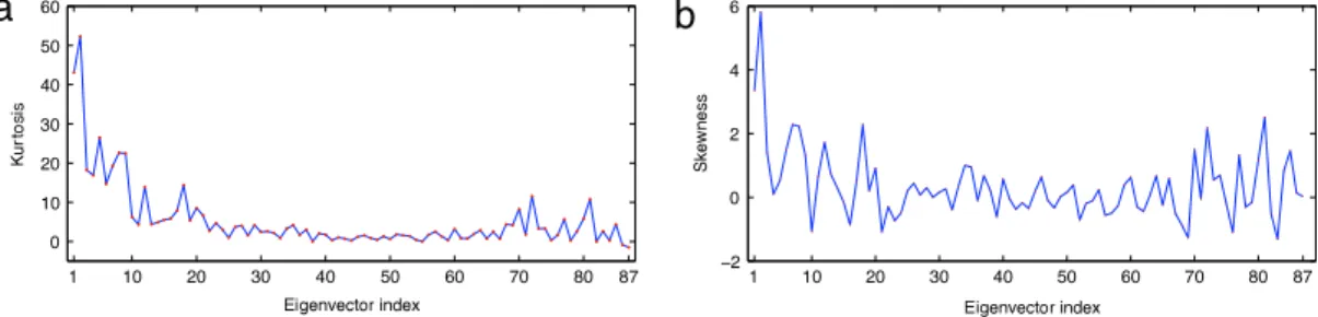
is almost uniform.

The kurtosis and skewness of the components of each

v

′

iare given inFig. 6. For the bulk, kurtosis and skewness fluctuate

around 3 and 0 respectively which is consistent with normal behavior.

Components of the

v

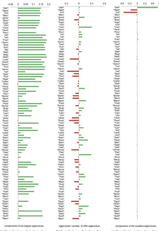
87suggest that most of the financial markets participate in this eigenvector. In addition, almost all

components are positive. To have a clear picture, we look atFig. 7showing the contributions of the stock markets to the

eigenvector corresponding to (a) the largest eigenvalue, (b) an eigenvalue from the bulk and (c) the smallest eigenvalue. For the largest eigenvalue, the majority of the markets have positive representations which is an indicative of a common factor

that affects almost all markets with the same bias. This gives us a reason to believe that

v

87represents a global market itself,

a

_b

Fig. 6. Kurtosis and skewness of the components of each eigenvector. 3.3. Global market mode

To see if

v

87represents a global market itself, we take the projection of the time series Ri

(

t

)

on the

v

87and compare it

with a standard measure of a global performance. In our case, the most related global index is the Morgan Stanley Capital International (MSCI) All Country World Index (ACWI). It is a free-float weighted equity index which includes both emerging

and developed world markets. The projection of the time series Ri

(

t

)

on

v

87is given by the following,

R_v87

(

t

) =

87



i=1

v

87,iRi

(

t

)

(13)

R_v87

(

t

)

is usually called the market mode [11,44] (in this study we will call it the global market mode).Fig. 8shows a

compar-ison of the global market mode and the returns of the MSCI index (we standardize both series to have zero mean and unit variance).

We find remarkable similarity between the two return series. The empirical correlation coefficient between them is

0.93. The good agreement shows that

v

87corresponds to a global market factor showing the general trend of all markets

and quantifies the worldwide influence on them [13].

Considering components of

v

87we see that the top six contributers are from European countries. On the other hand,

the majority of the markets have very small contributions that are proportional to the size and liquidity of these markets. An interesting case is the very small contributions of the big and liquid markets of South Korea, India and Russia. Since the market eigenvector can be considered as a general trend of all markets, this situation can be identified as the positive diversification of these emerging markets from others after the 2008 crisis.

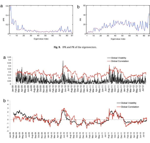
For each eigenvector, the number of markets with a significant participation can be accurately quantified by the IPR.Fig. 9

shows the IPR and PR as functions of the eigenvalue index. Eigenvectors corresponding to the bulk have participation ratios

around RMT prediction N

/

3

=

29. However,

v

87has the highest number (

≈

44) of significant participants which is far from

the suggested value. We also see that eigenvectors corresponding to the smallest eigenvalues have the lowest number of

significant participants.3

3.4. Relation between volatility and correlation

In order to examine the evolution of the correlations in the financial system, we investigate the mean correlation of

returns by a rolling window approach. We pick window length l

=

22 (business month) and roll the time window through

the data one day at a time. Explicitly, the mean correlationc

¯

l

(

t

)

for the correlation coefficients clij

(

t

)

in a time window

[t

−

l

+

1

,

t] is defined as

¯

cl

(

t

) =

2 N

(

N

−

1

)



i<j cl_ij

(

t

).

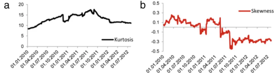
(14)

We want to compare the mean correlation of the financial markets with the system’s volatility. We take the absolute value of the global market mode as the daily volatility proxy of the financial system. A comparison of mean correlation and

volatility is given inFig. 10which shows that high levels of global volatility and correlation are strongly linked.4Furthermore,

after the times of high volatility, markets still stay highly correlated for some period5_{although we have to keep in mind that}

the procedure of shifting the window by one data point is partially responsible in this case.

3 That differs from the observations on the US stock market [11] where large values of PRs have been found at both edges of the theoretical distribution. 4 Other studies find similar results by empirical analyses [45–47] and agent based model simulations [48]. For example, Ref. [46] reveals that cross-correlations between nine highly developed markets fluctuate strongly with time and increase in periods of high market volatility. Moreover, based on this phenomenon, [49] constructs an indicator of systemic risk by principle component analysis.

5 In Ref. [50], such a situation is explained as the effect of the belief that market movement connectedness turns into a self-fulfilling prophecy after the crisis.

(a) Contributions of stock markets. (b) Contributions of stock markets. (c) Contributions of stock markets.

Fig. 7. Contributions of stock markets corresponding to different eigenvectors. The three highest volatility values are observed in the weeks of:

•

10/05/2010: European Union finance ministers agreed an emergency loan package that with IMF support could reach

750 billion euros to prevent a sovereign debt crisis spreading through the eurozone,

•

08/08/2011: Credit rating agency SP downgraded the US federal government rating from AAA (outstanding) to AA+

(excellent),

•

22/09/2011: Moody’s downgraded three US banks: Bank of America, Citigroup and Wells Fargo; SP downgraded seven

Italian banks and Fed announced significant downside risks to US economy, where each week above, global correlation also takes its highest values.

Fig. 8. MSCI All Country World Index returns vs. global market mode.

Fig. 9. IPR and PR of the eigenvectors.

a

b

Fig. 10. (a) Global volatility vs. global correlation and (b) global volatility (moving window) vs. global correlation.

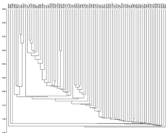
We also analyze the skewness and kurtosis of return distributions by rolling the time window of length l

=

264 (business

year) through the full data set (seeFig. 11, fat tails are demonstrated by excess kurtosis).

3.5. Time-varying largest eigenvalue

After revealing that the largest eigenvalue carries true information, we apply a similar approach of Ref. [51] to our data.

With a one-year length rolling window, we obtain the time-varying largest eigenvalue of the return correlation matrix and observe its characteristics.

Fig. 11. Kurtosis and skewness of returns obtained from a moving window.

Largest eigen

v

alue

Fig. 12. Time-varying largest eigenvalue of the correlation matrix obtained from a 1-year length rolling window.

Fig. 12shows that the largest eigenvalue peaks during the highest global volatility levels and there is a strong link between

the magnitude of this eigenvalue and the volatility levels in general.6

3.6. Correlation-based financial network analysis

Financial markets around the world can be regarded as a complex system. This forces us to focus on a global-level descrip-tion to analyze the interacdescrip-tion structure among markets which can be achieved by representing the system as a network. During the recent years networks have proven to be a very efficient way to characterize and investigate a wide range of

complex systems including stock, commodity and foreign exchange markets [45,52–76]. In this study, we are interested

in identifying the connection structure and hierarchy in the network of financial markets formed with cross-correlations of returns. In order to do that we construct the minimal spanning tree (MST) and the ultrametric hierarchical tree (UHT)

associated with it [44,45,53–80].

To create a network based on return correlations, we use the metric defined by Mantegna [53],

dij

=



2

(

1

−

cij

).

(15)

It is a valid euclidean metric since it satisfies the necessary properties; (i) dij

≥

0, (ii) dij

⇔

i

=

j, (iii) dij

=

djiand (iv)

dij

≤

dik

+

dkj. This transformation creates an N

×

N distance matrix D from the N

×

N cross-correlation matrix C. The

distance dijvaries from 0 to 2 with small distances corresponding to high correlations and vice versa.

MST is constructed as follows: start with the pair of elements with the shortest distance and connect them; then the second smallest distance is identified and added to the MST. The procedure continues until there are no elements left, with the condition that no closed loops are created. Finally we obtain a simply connected network that connects all N elements

with N

−

1 edges such that the sum of all distances is minimum.7

After defining the euclidean space of financial markets, we next move to the ultrametric space. An ultrametric space is

the space where all distances within it are ultrametric. The ultrametric distance d∗

ijis understood as a regular distance with

properties (i)–(iii) and property (iv) is replaced by a stronger condition; (iv)* d∗_ij

=

max

(

d∗_ik

,

d∗_kj

)

. Ultrametric distances are

important to hierarchical clustering since they redefine the distance between two elements as the distance between their

6 Which coincides with the findings of Ref. [51]: The authors study 1340 time series with 9 year daily data and investigate how the maximum singular valueλchanges over (time lags) for different years and find that it is greatest in times of crises.

7 This can be seen as a way to find the N−1 most relevant connections among a total of N(N−1)/2 connections which is especially appropriate for extracting the most important information concerning connections when a large number of markets is under consideration. In terms of financial markets, MSTs can also be considered as filtered networks enabling us to identify the most probable and the shortest path for the transmission of a crisis.

(a) 2005–2007 (period 1).

(b) 2009–2012 (period 2).

Fig. 13. Minimal spanning trees of (a) period 1 and (b) period 2.

closest ancestor. The MST provides the sub-dominant ultrametric hierarchical structure of the markets into what is called

UHT. The MST is associated with the single-linkage clustering algorithm [54], so we present the UHT using the same method.

To understand the effects of the 2008 financial crisis on markets’ integration structure, we analyze the cases correspond-ing to two different time periods; period one: 01/01/2005–01/01/2007 and period two: 01/01/2009–31/07/2012. The MSTs

and the UHTs of these periods are given inFigs. 13and14respectively.8

(a) 2005–2007 (period 1).

(b) 2009–2012 (period 2).

Table 1

Markets with highest node degrees. (a) Period 1 (b) Period 2

Market Node degree Market Node degree

France 11 France 11

Hong Kong 5 Hong Kong 5

Singapore 5 SP 5 Austria 5 Germany 5 Indonesia 4 Netherlands 4 Norway 4 Australia 4 SP 3 Singapore 3 UK 3 Qatar 3

South Korea 3 Kuwait 3

Australia 3 Slovenia 3

Table 2

Markets with highest node strength.

(a) Period 1 (b) Period 2

Market Node strength Market Node strength France 8.93286 France 7.88209

Austria 2.57976 SP 4.18860

SP 2.47343 Germany 3.79013

Hong Kong 2.26497 Netherlands 3.77997 Norway 2.13227 Hong Kong 3.77615 UK 2.10376 Australia 2.57149 Singapore 2.07421 Singapore 2.18214 Czech Republic 1.77035 Namibia 2.17670 South Korea 1.72229 Italy 1.80545 South Africa 1.47247 DJI 1.79151

For both periods, the three US market indexes are close together as expected and Germany serves as a hub for the con-nection between two main clusters; America and Europe. France seems to be the central node as it has the highest number of linkages in both cases and surprisingly the US market, which is usually accepted as the world’s most important finan-cial market, displays a somewhat looser connection with the others. The European Union (EU) seems to form the central trunk of the MSTs and the clusters appear to be organized principally according to a geographical position and historical

and linguistic ties [81].

However, major changes are observed between two periods. In particular, the effect of the eurozone debt crisis shows itself on the financial markets in period 2. The problematic countries Greece, Italy, Portuguese, Spain and Cyprus are all tied together, showing that bond market connection results with stock market connection. UK, not a eurozone member, loses its importance in the network in period 2. Three important markets that are positively diversified from the others through the 2008 crisis (Russia, India and South Korea) stand isolated in the network.

3.6.1. Centrality measures

In network theory, the centrality of a node determines the relative importance of that node within a network. Next, we

perform a detailed analysis on MSTs using different quantitative definitions of centrality.9

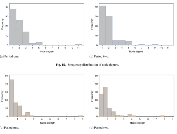
Node degree is the number of nodes that is adjacent to it in a network. In general the larger the degree, the more important

the node is. The highest ten node degrees and the frequency distributions are given inTable 1andFig. 15respectively.

Node strength is the sum of correlations of the given node with all other nodes to which it is connected. The highest ten

node strengths and the frequency distributions are given inTable 2andFig. 16respectively.

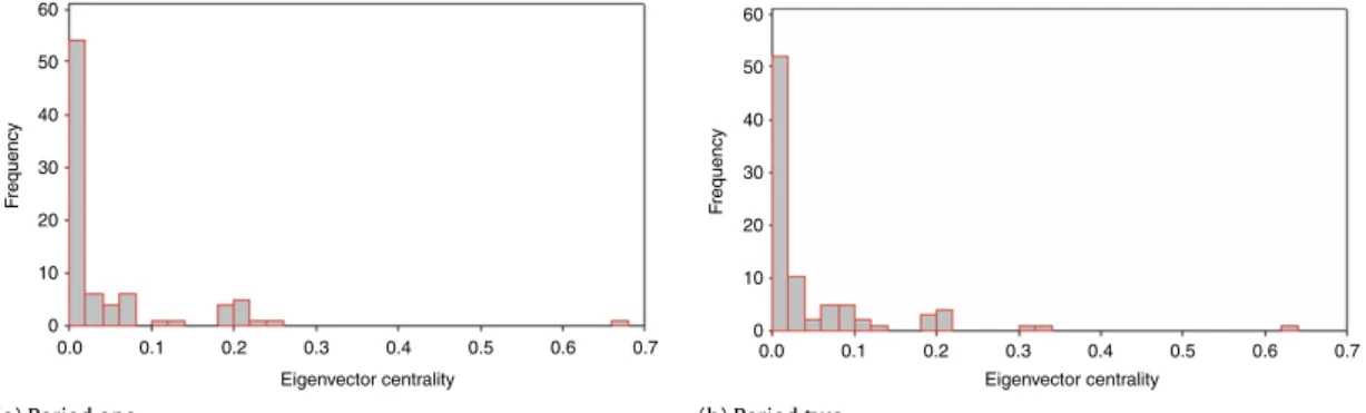
Eigenvector centrality is a measure that takes into account how important the neighbors of a node are. It is useful in particular when a node has a low degree but is connected to nodes with high degrees and thus the given node may influence

others indirectly. It is defined as the ith component of eigenvector v, where v corresponds to the largest eigenvalue

λ

of the

adjacency matrix A. The highest ten eigenvector centralities and the frequency distributions are given inTable 3andFig. 17

respectively.

9 Before beginning the analysis, we point out an important observation: even we have an extra three edges in the network in period two, the total distances in the MST is 82.593 whereas this values is 87.651 in period one. This shows increased strength in the correlation of financial markets after the 2008 crisis. A similar conclusion is obtained by using the time-varying correlation data from the Section3.4. In particular, we split the time-varying correlations into two sets as pre and post 2008. A non-parametric median comparison test reveals that the set of correlations in post 2008 has a significantly larger median.

0 1 2 3 4 5 6 7 8 9 10 11 Node degree 0 Node degree 1 2 3 4 5 6 7 8 9 10 11

(a) Period one. (b) Period two.

Fig. 15. Frequency distribution of node degree.

50 40 30 20 10 0 F requency 1 2 3 4 5 6 7 8 9 Node strength 50 40 30 20 10 0 F requency 1 2 3 4 5 6 7 8 9 Node strength

(a) Period one. (b) Period two.

Fig. 16. Frequency distribution of node strength.

Table 3

Markets with highest eigenvector centrality. (a) Period 1 (b) Period 2

Market Eigenvec. centrality Market Eigenvec. centrality

France 0.666 France 0.624 UK 0.249 Germany 0.323 Luxembourg 0.224 Netherlands 0.310 Germany 0.213 Austria 0.212 Belgium 0.212 Italy 0.212 Spain 0.212 UK 0.209 Sweden 0.210 Finland 0.209 Finland 0.210 Switzerland 0.190 Switzerland 0.193 Belgium 0.190 Netherlands 0.193 Ireland 0.190

Betweenness centrality measures the importance of a node as an intermediate part between other nodes. For a given node k, it is defined as B

(

k

) =



i,j nij

(

k

)

mij (16)

where nij

(

k

)

is the number of shortest geodesic paths between nodes i and j passing through k, and mijis the total number

of shortest geodesic paths between i and j.10_{The highest ten betweenness centralities and the frequency distributions are}

given inTable 4andFig. 18respectively.11

10 MST is a fully-connected network so mij̸=0.

11 There are 38 indexes in period one and 41 indexes in period two with zero betweenness centrality i.e. for any two markets in the network, no shortest path passes through them.

60 50 40 30 20 10 0 F requency 0.0 0.1 0.2 0.3 0.4 0.5 0.6 0.7 Eigenvector centrality 60 50 40 30 20 10 0 F requency 0.0 0.1 0.2 0.3 0.4 0.5 0.6 0.7 Eigenvector centrality

(a) Period one. (b) Period two.

Fig. 17. Frequency distribution of eigenvector centrality.

F requency Betweenness centrality 60 70 50 40 30 20 10 0 0.0 0.1 0.2 0.3 0.4 0.5 0.6 0.7 F requency Betweenness centrality 60 70 50 40 30 20 10 0 0.0 0.1 0.2 0.3 0.4 0.5 0.6 0.7

(a) Period one. (b) Period two.

Fig. 18. Frequency distribution of betweenness centrality. Table 4

Markets with highest betweenness centrality. (a) Period 1 (b) Period 2

Market Btw. centrality Market Btw. centrality France 0.7249486 France 0.68044 Hong Kong 0.5166030 Namibia 0.57264 Austria 0.5145460 Netherlands 0.53953 UK 0.4757567 South Africa 0.50150 Luxembourg 0.4601822 Singapore 0.46539 Czech Republic 0.3385248 Hong Kong 0.45253 South Korea 0.2970908 Australia 0.29521 Hungary 0.2876873 Germany 0.28810 Egypt 0.2535998 Austria 0.27579 Singapore 0.2248016 Czech Republic 0.25964

Closeness centrality is a measure of the average geodesic distance from one node to all others. This measure is high for strongly connected central nodes and large for poorly connected ones. For node i in a network with N nodes, it is defined as

C

(

i

) =

1 N



j=1 d

(

i

,

j

)

(17)

where d

(

i

,

j

)

is the minimum geodesic path distance between nodes i and j. The highest ten closeness centralities and the

frequency distributions are given inTable 5andFig. 19respectively.

Analysis reveals that France takes first place in almost all categories for both periods and other financial centers Germany, Hong Kong and Singapore keep their importance in the network after the crisis. However, the same cannot be said for the UK; while belonging to the top ten in all categories in period one, it belongs to the top ten only in 2 categories in period

two.12

12 Note that all frequency distributions of centrality measures (except for closeness centrality) are likely to decrease exponentially. One may say that these measures exhibit a power-law distribution; p(x) ∼x−β_{for measure value x and constantβwhich in the case the network is called scale-free [82].}

Germany 0.002252 Germany 0.002058 Belgium 0.002203 Austria 0.002058

Spain 0.002203 Italy 0.001976

Sweden 0.002193 Hong Kong 0.001961

Finland 0.002193 UK 0.001953 12 10 8 6 4 2 0 F requency 0.0010 0.0015 0.0020 0.0025 Closeness centrality F requency Closeness centrality 12 10 8 6 4 2 0 0.0010 0.0015 0.0020 0.0025

(a) Period one. (b) Period two.

Fig. 19. Frequency distribution of closeness centrality.

4. Discussion

In our study, one concern about the correlations between financial markets is that the relationship may be non-linear; in that case rank correlation may capture the relations better. In order to see the difference, we use a rank correlation approach:

for each index i, the returns Ri

(

t

)

are ranked Rranki

(

t

)

then normalized as

r_irank

(

t

) ≡

R rank i

− ⟨

Rranki

⟩

σ

rank i (18) where

σ

rank i

≡



⟨

(

Rrank

i

)

2

⟩ − ⟨

Rranki

⟩

2; then we repeat every analysis. The results are almost indistinguishable. The largest

eigenvalue is

≈

22

.

44 and

≈

94% of the eigenvalues are smaller than

λ

max. Considering components of the largest eigenvector,

the top six positive contributers do not change.

For the network analysis, we define the metric as a linear realization of the rank correlation; dij

=

1

−

cij. The major

difference is that (instead of Germany) France serves as a hub for connecting North America and Europe in period two. 4.1. Further study

A lagged relationship is a possible characteristic of many pairwise financial time series. First, it would not be a surprise if one series had a delayed response to another time series, or it had a delayed response to a common event that affects both series. Secondly, it may be the case that the response of one series to the other or to an outside event may spread in time, such that an event restricted to one observation elicits a response at multiple observations. Furthermore, series may not even be stationary in some cases. Equal-time cross-correlations are inadequate to characterize the relationship between time series in such situations. Some authors incorporated these facts into their studies and revealed interesting results using

the concepts of detrended and long-range cross-correlations and time lag RMT [83–89].13_{In the near future, we are planning}

to apply these new approaches to our data set and analyze the differences in our findings.

13 For example, Kullmann et al. [83] showed that in many cases the maximum correlation appears at nonzero time shift, indicating directions of influence between the stocks. Similarly, Wang et al. [84] find long-range power-law cross-correlations in the absolute values of returns that quantify risk, and find that they decay much more slowly than cross-correlations between the returns. They find that when a market shock is transmitted around the world, the risk decays very slowly.

5. Conclusion

The global financial crisis of 2008 began in July 2007 when a loss of confidence by investors in the value of securi-tized mortgages in the US resulted in a liquidity crisis. In September 2008, the crisis deepened as stock markets world-wide crashed and entered a period of high volatility. This study compares before and after the 2008 crisis by analyzing the cross-correlations of financial markets using the tools of RMT and network theory.

In particular, we verified the validity of the universal predictions of RMT for the statistics of the eigenvalues and the corre-sponding eigenvectors of the cross-correlation matrix. Then the cross-correlations between markets not totally explainable by randomness were identified by computing the deviations of the empirical data from the RMT predictions. We showed the presence of a certain linear combination of indexes representing a global market itself that arises from interactions.

By using this particular combination, we observed that markets become highly correlated in times of high volatility (also the time-varying largest deviating eigenvalue peaks during the highest volatility); moreover when the volatility passes to its low levels, the increased degree of co-movement continues for a considerable amount of time. We also find that markets are more correlated after 2008 compared to the period of 2005–2007. These facts lower the diversification potential even if one constructs a widely internationally diversified portfolio of stocks.

We found the connection structure of financial markets for pre and post 2008 crisis using correlation based networks. We show that in an environment of increasing integration of trade and financial markets, geographical position and historical and linguistic ties still play an important role in co-movements of stock markets. Analysis also shows that eurozone debt crisis forces the stock markets of problematic countries to move together, revealing an interesting fact on how bond and stock markets of a country interact.

We identified key financial markets using several centrality measures. Analysis shows that centers like France, Germany and Hong Kong keep their importance in the financial system after the 2008 crisis. However, the same cannot be said for the UK.

To extract the information arising from non-linear relations between markets, we repeated each analysis using a rank correlation and found that the results are almost indistinguishable. Possible extensions for further research includes appli-cations of the long-range cross-correlations and time lag-RMT to our data.

Acknowledgments

We thank the anonymous referees for helpful comments and suggestions that significantly improved this paper.

Appendix. Analyzed markets

Country Index Symbol

Argentina Merval Arge

Australia SP/ASX 200 Aust

Austria ATX Autr

Bahrain Bahrain all share index Bahr

Bangladesh DSE general index Bang

Belgium BEL 20 Belg

Brazil Ibovespa Braz

Bosnia and Herzegovina SASE 10 BoHe

Botswana Gaborone Bots

Bulgaria SOFIX Bulg

Chile IPSA Chil

China Shangai SE composite Chin

Colombia IGBC Colo

Croatia CROBEX Croa

Cyprus CSE Cypr

Czech Republic PX CzRe

Denmark OMX Copenhagen 20 Denm

Egypt EGX 30 Egyp

Estonia OMXT Esto

Finland OMX Helsinki Finl

France CAC 40 Fran

Germany DAX Germ

Ghana Ghana all share index Ghan

Greece Athens SX general index Gree

Hong Kong Hang Seng HoKo

Jamaica Jamaica SX market index Jama

Japan Nikkei 225 Japa

Jordan ASE general index Jord

Kazakhstan KASE Kaza

Kenya NSE 20 Keny

Kuwait Kuwait SE weighted index Kwai

Latvia OMXR Latv

Lebanon BLOM Leba

Lithuania OMXV Lith

Luxembourg Luxembourg LuxX Luxe

Macedonia MBI 10 Mace

Malaysia KLCI Mala

Malta Malta SX Index Malt

Mauritius SEMDEX Maur

Mexico IPC Mexi

Mongolia MSE TOP 20 Mong

Montenegro MOSTE Mont

Morocco CFG 25 Moro

Namibia FTSE/Namibia overall Nami

Netherlands AEX Neth

New Zealand NZX 50 NeZe

Nigeria Nigeria SX all share index Nige

Norway OBX Norw

Oman MSM 30 Ohma

Pakistan Karachi 100 Paki

Peru IGBVL Peru

Philippines PSEi Phil

Poland WIG Pola

Portugal PSI 20 Port

Qatar DSM 20 Qata

Romania BET Roma

Russia MICEX Russ

Saudi Arabia TASI SaAr

Serbia BELEX 15 Serb

Singapore Straits times Sing

Slovakia SAX Slok

Slovenia SBI TOP Slov

South Africa FTSE/JSE Africa all share SoAf

South Korea KOSPI SoKo

Spain IBEX 35 Spai

Sri Lanka Colombo all-share index SrLa

Sweden OMX Stockholm 30 Swed

Switzerland SMI Swit

Taiwan TAIEX Taiw

Thailand SET Thai

Tunisia TUNINDEX Tuni

Turkey ISE national 100 Turk

Ukraine PFTS Ukra

United Arab emirates ADX general index UAE

United Kingdom FTSE 100 UK

United States of America Dow Jones industrial DJI

Country Index Symbol

United States of America Nasdaq composite Nasd

United States of America SP 500 SP

Venezuela IBC Vene

Vietnam VN-Index Viet

References

[1]L.H. Ederington, J.H. Lee, J. Finance 48 (1993) 1161.

[2]P. Balduzzi, E.J. Elton, T.C. Green, J. Financ. Quant. Anal. 36 (2001) 53. [3]T.G. Andersen, T. Bollerslev, F.X. Diebold, C. Vega, J. Int. Econ. 73 (2007) 251. [4]H. Markowitz, J. Finance 7 (1952) 77.

[5]V. Plerou, P. Gopikrishnan, B. Rosenow, L.A.N. Amaral, H.E. Stanley, Physica A 287 (2000) 374. [6]M. Mehta, Random Matrices, Academic Press, 1994.

[7]J. Shen, B. Zheng, EPL 86 (2009) 48005.

[8]B. Rosenow, P. Gopikrishnan, V. Plerou, H.E. Stanley, Physica A 314 (2002) 762. [9]B. Rosenow, P. Gopikrishnan, V. Plerou, H.E. Stanley, Physica A 324 (2003) 241. [10]L. Laloux, P. Cizeau, J.P. Bouchaud, M. Potters, Phys. Rev. Lett. 83 (1999) 1467.

[11]V. Plerou, P. Gopikrishnan, B. Rosenow, L.A.N. Amaral, T. Guhr, H.E. Stanley, Phys. Rev. E 65 (2001) 066126. [12]D. Wilcox, T. Gebbie, Physica A 375 (2007) 584.

[13]V. Plerou, P. Gopikrishnan, B. Rosenow, L.A.N. Amaral, H.E. Stanley, Phys. Rev. Lett. 83 (1999) 1471.

[14]J.P. Bouchaud, M. Potters, Financial applications of random matrix theory: a short review, in: G. Akemann, J. Baik, P.D. Francesco (Eds.), Handbook on Random Matrix Theory, Oxford University Press, 2011.

[15]J.P. Bouchaud, G. Biroli, M. Potters, Europhys. Lett. 78 (2007) 10001.

[16]L. Laloux, P. Cizeau, M. Potters, J.P. Bouchaud, Int. J. Theor. Appl. Finance 3 (2000) 391. [17]V. Plerou, P. Gopikrishman, B. Rosenow, L.A.N. Amaral, H.E. Stanley, Phys. Rev. E 60 (1999) 5306. [18]B. Rosenow, V. Plerou, P. Gopikrishnan, L.A.N. Amaral, H.E. Stanley, Int. J. Theor. Appl. Finance 3 (2002) 399. [19]V. Kulkarni, N. Deo, Eur. Phys. J. B 60 (2007) 101.

[20]J. Kwapien, S. Drozdz, A.Z. Gorski, P. Oswiecimka, Acta Phys. Pol. B 37 (2006) 3039. [21]M. Potters, J.P. Bouchaud, L. Laloux, Acta Phys. Pol. B 36 (2005) 2767.

[22]J.P. Bouchaud, L. Laloux, M.A. Miceli, M. Potters, Eur. Phys. J. B 2 (2007) 201. [23]R. Rak, S. Drozdz, J. Kwapien, P. Oswiecimka, Acta Phys. Pol. B 37 (2006) 3123. [24]A.C.R. Martins, Physica A 379 (2007) 552.

[25]A.C.R. Martins, Physica A 383 (2007) 527. [26]R.K. Pan, S. Sinha, Phys. Rev. E 76 (2007) 1.

[27]I.I. Dimov, P.N. Kolm, L. Maclin, D.Y.C. Shiber, Quant. Finance 12 (2012) 567. [28]J.D. Noh, Phys. Rev. E 61 (2000) 5981.

[29]R. Rak, J. Kwapien, S. Drozdz, P. Oswiecimka, Acta Phys. Pol. A 114 (2008) 561. [30]T. Conlon, H.J. Ruskin, M. Crane, Physica A 388 (2009) 705.

[31]M.C. Munnix, R. Schafer, T. Guhr, Physica A 389 (2010) 767. [32]A. Namaki, G.R. Jafari, R. Raei, Physica A 390 (2011) 3020.

[33]G. Oh, C. Eom, F. Wang, W.S. Jung, H.E. Stanley, S. Kim, Eur. Phys. J. B 79 (2011) 55. [34]A. Namaki, A.H. Shirazi, R. Raei, G.R. Jafari, Physica A 390 (2011) 3835.

[35]S. Maslov, Physica A 301 (2001) 397.

[36]S. Drozdz, F. Grummer, F. Ruf, J. Speth, Physica A 294 (2001) 226. [37]L.S. Junior, I.P. Franca, Physica A 391 (2012) 187.

[38]T.H. Baker, P.J. Forester, P.A. Pearce, J. Phys. A: Math. Gen. 31 (1998) 6087. [39]A. Edelman, SIAM J. Matrix Anal. Appl. 9 (1998) 543.

[40]A.M. Sengupta, P.P. Mitra, Phys. Rev. E 60 (1999) 3389.

[41]T.A. Brody, J. Flores, J.B. French, P.A. Mello, A. Pandey, S.S.M. Wong, Rev. Modern Phys. 53 (1981) 385. [42]T. Guhr, A. Muller-Groeling, H.A. Weidenmuller, Phys. Rep. 299 (1998) 190.

[43]V. Plerou, P. Gopikrishnan, L.A.N. Amaral, M. Meyer, H.E. Stanley, Phys. Rev. E 60 (1999) 6519. [44]P. Gopikrishnan, B. Rosenow, V. Plerou, H.E. Stanley, Phys. Rev. E 64 (2001) 035106. [45]J.P. Onnela, A. Chakraborti, K. Kaski, J. Kertesz, A. Kanto, Phys. Rev. E 68 (2003) 056110. [46]B. Solnik, C. Bourcrelle, Y. Le Fur, Financ. Anal. J. 52 (1996) 17.

[47]C.B. Erb, C.R. Harvey, T.E. Viscanta, Financ. Anal. J. 50 (1994) 32. [48]B. LeBaron, W.B. Arthur, R. Palmer, J. Econ. Dyn. Control 23 (1999) 1487.

[49] Z. Zheng, B. Pobodnik, L. Feng, B. Li, Nature Scientific Reports 2.http://dx.doi.org/10.1038/srep00888. [50]M. Dalkir, Financ. Res. Lett. 6 (2009) 23.

[51]B. Podobnik, D. Wang, D. Horvatic, I. Grosse, H.E. Stanley, EPL 90 (2010) 68001.

[52]M. Tuminello, T. Aste, T. DiMatteo, R.N. Mantegna, Proc. Natl. Acad. Sci. USA 102 (2005) 10421. [53]R.N. Mantegna, Eur. Phys. J. B 11 (1999) 193.

[54]M. Tumminello, T. Aste, T.D. Matteo, R.N. Mantegna, Eur. Phys. J. B 55 (2007) 209. [55]G. Bonanno, F. Lillo, R.N. Mantegna, Quant. Finance 1 (2001) 96.

[56]S. Micchiche, G. Bonanno, F. Lillo, R.N. Mantegna, Physica A 324 (2003) 66. [57]J.P. Onnela, A. Chakraborti, K. Kaski, J. Kertesz, Physica A 324 (2003) 247. [58]J.P. Onnela, A. Chakraborti, K. Kaski, J. Kertesz, A. Kanto, Phys. Scr. T 106 (2003) 48. [59]J.P. Onnela, K. Kaski, J. Kertesz, Eur. Phys. J. B 38 (2004) 353.

[60]G. Bonanno, G. Caldarelli, F. Lillo, S. Micciche, N. Vandewalle, R.N. Mantegna, Eur. Phys. J. B 38 (2004) 363. [61]C. Borghesi, M. Marsili, S. Micciche, Phys. Rev. E 76 (2007) 026104.

[62]J.G. Brida, W.A. Risso, Physica A 387 (2008) 5205.

[63]Y. Zhang, G.H.T. Lee, J.C. Wong, J.L. Kok, M. Prusty, S.A. Cheong, Physica A 390 (2011) 2020. [64]M. Tumminello, F. Lillo, R.N. Mantegna, J. Econ. Behav. Organ. 75 (2010) 40.

[65] S. Droyzdyz, J. Kwapien, J. Speth, AIP Conf. Proc., 1261, 2010, p. 256.

[66]C. Coronnello, M. Tumminello, F. Lillo, S. Micchiche, R.N. Mantegna, Acta Phys. Pol. B 36 (2005) 2653. [67]R. Coelho, C.G. Gilmore, B. Lucey, P. Richmond, S. Hutzler, Physica A 376 (2007) 455.

[79]M. Tumminello, F. Lillo, R.N. Mantegna, Phys. Rev. E 76 (2007) 031123. [80]M. Tumminello, F. Lillo, R.N. Mantegna, Acta Phys. Pol. B 38 (2007) 4079. [81]C.G. Gilmore, B.M. Lucey, M.W. Boscia, Physica A 389 (2010) 4875. [82]A.L. Barabsi, R. Albert, H. Jeong, Physica A 272 (1999) 173. [83]L. Kullmann, J. Kertesz, K. Kaski, Phys. Rev. E 66 (2002) 026125.

[84]D. Wang, B. Podobnik, D. Horvatic, H.E. Stanley, Phys. Rev. E 83 (2011) 046121. [85]B. Podobnik, D. Wang, D. Horvatic, I. Grosse, H.E. Stanley, EPL 90 (2010) 68001.

[86] S. Arianos, A. Carbone, J. Stat. Mech. (2009) 03037. URLhttp://dx.doi.org/10.1088/1742-5468/2009/03/P03037. [87]B. Podobnik, D.F. Fu, H.E. Stanley, P. Ivanov, Eur. Phys. J. B 56 (2007) 47.

[88]B. Podobnik, I. Grosse, D. Horvatic, S. Ilic, P. Ivanov, H.E. Stanley, Eur. Phys. J. B 71 (2009) 243. [89]B. Podobnik, D. Horvatic, A.M. Petersen, H.E. Stanley, Proc. Natl. Acad. Sci. USA 106 (2009) 22079.