ORIGINAL RESEARCH PAPER
A statistical assessment on global drift ratio demands
of mid‑rise RC buildings using code‑compatible real
ground motion records
Mehmet Palanci1 · Ali Haydar Kayhan2 · Ahmet Demir2
Received: 4 August 2017 / Accepted: 1 May 2018 / Published online: 21 May 2018 © Springer Science+Business Media B.V., part of Springer Nature 2018
Abstract Over the past 20 years, significant socio-economic losses have been
encoun-tered in Turkey due to several moderate to large earthquakes. The studies published after the earthquakes concurringly emphasized that multistory reinforced concrete (RC) build-ings, mostly 3–7 story ones, collapsed or were heavily damaged as a result of inadequate seismic performance. Global drift ratio demands are mostly used as a representative quan-tity for determining the behavior of structures when subjected to earthquakes. In this study, three representative mid-rise RC buildings are analyzed by nonlinear time history analysis using code-compatible real ground motion record sets and the calculated global drift ratio demands of these buildings are statistically evaluated. Ground motion record sets com-patible with the design spectrum defined for local soil classes in the Turkish Earthquake Code (TEC-2007) are used for the analyses. In order to evaluate the effect of the number of ground motions on drift ratio demands, five different ground motion record sets with 7, 11 and 15 ground motion records are used separately for each local soil class. Results of this study indicate that (1) the dispersion of global drift ratio demands calculated for individual ground motion records in record sets is high, (2) local soil class has no significant effect on dispersion. However, dispersion increases in a direct proportion to the number of ground motion records in a record set, (3) the mean of global drift ratio demands calculated for different ground motion record sets may differ although they are compatible with the same design spectrum, (4) the mean of the drift demands obtained from different ground motion record sets compatible with a particular design spectrum can be accepted as simply random samples of the same population at 95% confidence level.
* Mehmet Palanci
[email protected] Ali Haydar Kayhan [email protected]
Ahmet Demir [email protected]
1 Department of Civil Engineering, Istanbul Arel University, Istanbul, Turkey 2 Department of Civil Engineering, Pamukkale University, Denizli, Turkey
Keywords RC buildings · Nonlinear dynamic analysis · Statistical evaluation
1 Introduction
One of the largest potential sources of casualties and damage for inhabited areas due to natural hazard is earthquakes. Every year, many earthquakes varying in size and destruc-tive potential occur worldwide. Earthquakes, especially moderate and large ones can cause serious socio-economic losses. The amount of socio-economic losses that result from an earthquake depends on the size, depth and location of the earthquake, the intensity of the ground shaking and related effects on the building inventory, and the vulnerability of that building inventory to damage.
Turkey is a country under the threat of damaging earthquakes and over the past 20 years significant socio-economic losses have occurred resulting from several moderate and large earthquakes, such as 1998 Adana–Ceyhan (Ms = 6.3), 1999 Kocaeli (Mw = 7.4), 1999
Düzce (Mw = 7.2), 2002 Afyon–Sultandagi (Mw = 6.3), 2003 Bingöl (Mw = 6.4) and 2011
Van (Mw = 7.2). The studies published after these earthquakes regarded the seismic
per-formance of the buildings, the observed structural damages and the reasons for these dam-ages (Sezen et al. 2000; Adalier and Aydingun 2001; Akkar et al. 2005a; Celep et al. 2011; Taskin et al. 2013; Yon et al. 2013; Korkmaz 2015). These studies concurringly empha-sized that multistory RC buildings, especially 3–7 story ones collapsed or were heavily damaged due to inadequate seismic performance. The main reasons for the observed dam-ages can be classified as poor concrete quality, insufficient reinforcement detailing, soft and weak story mechanisms, short column problems, insufficient shear walls, large and heavy overhangs, strong beams-weak columns and poor construction practices (Inel et al. 2008; Arslan 2010; Ilki and Celep 2012). The observed insufficient seismic performance and structural properties of the existing RC buildings after major earthquakes showed that there is a critical discrepancy between the presence of seismic code regulations and the existing situation. This outcome is mainly based on the lack of influential control mechanisms for the design and construction practices (Ilki and Celep 2012). The experiences gained from the evaluation of the studies may be very useful for predicting the expected behavior of existing buildings in future earthquakes and taking the necessary measures to reduce pos-sible damages and losses.
Recently, performance based design methods have been used extensively for the seismic design or evaluation of buildings. Design criteria are expressed in terms of achieving stated performance objectives when the structure is subjected to stated levels of seismic hazard. Thus, performance objectives, determination of seismic demands and performance evalu-ation are three principal steps of the performance based design. The SEAOC Vision 2000 document (SEAOC Vision 2000 Committee 1995), one of the first major documents on performance based design, listed various advanced performance based design or evalua-tion approaches such as (a) displacement-based design, (b) energy-based design and (c) comprehensive design considering lifecycle cost. So far, the displacement based design approach has been widely adopted and structures are being designed in accordance with target response parameters such as maximum displacement, ductility demand, global and inter-story drift ratio etc. (Priestley et al. 2007). The same parameters are also used to define various performance levels or limit states (ATC-40 1996; FEMA-440 2005).
Among the target response parameters, global and inter-story drift ratio demands can be accepted as the most commonly used ones. One of the most important steps in performance
based design and/or the evaluation of structures is the determination of demands for seis-mic loads related to considered seisseis-mic level and this requires accurate structural modeling and analysis. A nonlinear time history analysis of a three-dimensional structural model is the most comprehensive and accurate analytical method to evaluate the seismic demands. Nowadays, this analysis method has been increasingly preferred because of the develop-ments in the processing power of computers and the software industry. However, a nonlin-ear time history analysis of three-dimensional structures is complex. For this reason, the simpler two-dimensional frames (Akkar et al. 2005b; Medina and Krawinkler 2005; García and Miranda 2006; Hatzigeorgiou and Liolios 2010; García and Miranda 2010; Ghaffarza-deh et al. 2013) or single degree of freedom (SDOF) systems (Bazzurro and Luco 2005; D’Ambrisi and Mezzi 2005; García and Miranda 2007; Lin and Miranda 2009; Hatzigeor-giou and Beskos 2009; Hou and Qu 2015) are also preferred as structural analysis models. In these studies, different criteria are used in the selection of ground motion records for nonlinear time history analyses.
It should be noted that ground motion records affect the seismic demands used for seismic design and/or performance evaluation (Katsanos et al. 2010; Araújo et al. 2016). Therefore, it is important to use suitable ground motion records for time history analyses, based on the seismicity and local soil conditions of a structure to make a reliable estima-tion of the seismic demands (Iervolino et al. 2010a; Han et al. 2014). In order to perform a time history analysis, relatively similar procedures with minor different requirements are described in modern seismic codes (TEC-2007 2007; FEMA-368 2001; EUROCODE-8 2004; ASCE 07-05 2006; GB 2010). For example, synthetic, artificial, or real ground motion records could be used as long as they are compatible with regional design spec-tra defined in the seismic codes within a stated period range. Usually, according to these codes at least three ground motion records are required. The average of the structural responses can be used for seismic design and/or performance evaluation if at least seven ground motion records are selected, otherwise the maximum of structural responses should be considered.
In modern seismic design codes, the ground motion selection process only considers the average spectrum of the selected ground motions for time history analysis and the tar-get design spectrum without considering random variability of the ground motion records. In addition, recent studies showed that it is possible to obtain different code-compatible ground motion record sets by selecting and scaling from hundreds of ground motion records available in digital databases (Iervolino et al. 2008; Kayhan et al. 2011; Kayhan 2016). Hence, estimated seismic demands representing the structural responses to seismic excitation vary significantly and could be accepted as random variables that change accord-ing to code-compatible record sets used for nonlinear time history analyses (Cantagallo et al. 2014; Macedo and Castro 2017). Recently, various studies were carried out to investi-gate the efficiency of the selecting and scaling of ground motion records according to vari-ous seismic codes. Reyes and Kalkan (2012) used theoretical models with varying lateral strength reduction factors (R) and natural vibration periods to evaluate the accuracy of the ground motion scaling procedure of ASCE 07-10 (2010) in terms of structural responses and as a result they observed high variations. Katsanos and Sextos (2013) developed an integrated software environment to select structure specific ground motions according to the European and US seismic codes and applied it to irregular RC buildings. Results of this study have demonstrated the very high variability in both structural and member responses. Sextos et al. (2011) used the EUROCODE-8 based earthquake record selection procedure for the evaluation, considering the irregular damaged RC buildings and highlighted the large dispersion and demonstrated the limitations of the EUROCODE-8 earthquake ground
motion selection framework for the assessment of both elastic and inelastic structural response of multi-story irregular RC buildings. Kayhan and Demir (2016) used two dimen-sional generic RC frames to evaluate the code-compatible procedure of the TEC-2007 in different soil conditions using roof and inter-story drift ratios by various record sets that have seven ground motions. According to Kayhan and Demir, the variation of seismic demands and inter-story drift ratios are significantly high. Shome et al. (1998) pointed out that the number of records required to obtain an estimate of the median response to within a defined confidence interval depends on the standard deviation of the response. There-fore, the number of records to be used should depend on both the procedure used to select and scale the accelerograms and the nature of the structural response being investigated. Hancock et al. (2008) stated that the number of required records and the degree of bias both systematically decrease as one applies more constraint on the scaling and matching of accelerograms. Hence, the number of records that are required to obtain a robust esti-mate of the inelastic response may be significantly reduced through the use of the spec-trally matched, wavelet-adjusted, accelerograms. Hancock et al. also stated that the degree of bias may be accounted for through the use of factors as commonly adopted elsewhere in seismic design codes.
The aim of this study is to investigate the effect of the code-based record selection meth-ods on the global drift ratio demands of RC buildings in terms of mean and variation cal-culated by nonlinear time history analyses using different code-compatible sets of ground motion records. The effect of local soil conditions and the number of ground motions in the record sets used for the nonlinear time history analyses on drift ratio demands is also inves-tigated. In accordance with these aims, three mid-rise RC buildings that represent a major portion of the existing RC building stock in Turkey are considered. Five ground motion record sets with 7, 11 and 15 ground motion records are used separately for the nonlin-ear time history analysis of the buildings considering various local soil classes defined in the TEC-2007. The lateral strength and displacement capacity of the buildings are deter-mined by pushover analyses and the dynamic characteristics of the buildings are repre-sented by equivalent SDOF systems. The maximum drift ratio demands using individual ground motion records in the record sets and the mean and the coefficient of variation of the demands are calculated. A one way analysis of variance (ANOVA) is performed to evaluate the differences between the mean drift ratios demands calculated for different record sets compatible with the same design spectrum. Finally, the sampling distributions of the mean drift ratio demands are estimated for the buildings considering different local soil classes. Using the results of this study, various recommendations are suggested and also practical implications in the selecting and scaling of seismic codes in the assessment and design of structures are also discussed for practitioners in civil engineering.
2 The representative RC buildings
In the present study, existing mid-rise buildings in Turkey are represented by a selection of three 5-story RC buildings, namely 5A, 5B and 5C. These buildings are typical RC frame buildings consisting of columns and beams without structural walls. The selected mid-rise RC buildings were designed in accordance with TEC-1975 and represent the general characteristics of existing RC buildings in Turkey. The nonlinear behavior of the selected buildings are determined by using 3-D nonlinear structural models and the required struc-tural properties (cross-sectional dimensions of members, reinforcement details, filled walls,
dead and moving loads on slabs, etc.) are obtained from their own architectural and RC design projects.
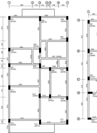
The floor plans for buildings 5A and 5C are given in Fig. 1 and the floor plan for build-ing 5B is given in Fig. 2. For building 5A, the height of the base story is 3.40 m, the first story is 3.00 m and the rest of the stories are 2.80 m. The cross-sectional dimension of the beams in all story plans is 0.20 × 0.50 m except K05 (0.20 × 0.60 m). The cross-sectional dimensions of the columns at the base story are given in Fig. 1. The longitudinal reinforce-ment ratio of the columns varies between 0.8 and 1.1%. The cross-sectional dimensions of some of the columns are reduced on the upper floors. It can be seen from Fig. 1 that all the columns are placed in the direction of the strong inertia (along y direction). This situ-ation is also observed in significant parts of the existing structures in Turkey and it can be considered as a design mistake. Furthermore, three continuous moment-resisting frames can be seen along y direction but most of the frames along x direction are discontinuous. Continuous moment-resisting frames are the main part of the seismic force-resisting sys-tems in buildings. As understood, building 5A has serious shortcomings in the x direction compared to the y direction in terms of both the placement of structural members and the continuous moment-resisting frames.
For building 5B, the height of the base story is 3.50 m and the other floors are 2.80 m. The cross-sectional dimensions of the beams on all floors are 0.25 × 0.60 m. The
cross-sectional dimensions of the columns at the base story are given in Fig. 2. The longi-tudinal reinforcement ratio of the columns is around 1.0–1.1%. The cross-sectional dimen-sions of the beams and columns are the same for the upper floors.
The height of all the stories in building 5C is 2.80 m. The cross-sectional dimensions of the beams are 0.20 × 0.50 m except for K28 and K29 which are 0.20 × 0.60 m. The cross-sectional dimensions of the beams on the upper stories are the same as the base story. The longitudinal reinforcement ratio of the columns ranges between 1.0 and 1.5%. The cross-sectional dimensions of the columns are reduced on the upper floors as in building 5A. It can be seen from Fig. 1 that apart from the outer axis there is only one continuous moment-rising frame which is the axis D.
Most of the buildings constructed in accordance with the TEC-1975 are designed using C16 class concrete (fc = 16 MPa) and S220 class reinforcement steel (fy= 220 MPa). It is
also observed that C16 and S220 class materials were used in the design projects of the selected representative buildings. For this reason, C16 and S220 materials are taken into Fig. 2 Floor plan of building 5B (units in cm)
consideration for the structural model of the selected representative buildings. In the TEC-1975 and the more recent seismic design codes, various regulations such as the detailing transverse reinforcement of structural members, confinement regions at the end of struc-tural members and beam-column connections are considered. However, it is a well-known fact that before the TEC-1997 there was non-compliance with these requirements in con-struction (Arslan 2010; Bal et al. 2008). For instance, at the ends of columns and beams, the stirrup spacing is expected to be equal to or smaller than 100 mm. Thus, in order to represent the insufficient transverse reinforcement of structural members, stirrup spacing is determined as 200 mm in the analysis of the representative buildings. The diameter of the stirrup for columns and beams is 8 mm. In the analysis models, dead and live loads, and the self-weight of beams, walls and slabs are taken into consideration.
2.1 Modeling approach
In this part of the study, information about the 3-D nonlinear analysis models of the rep-resentative buildings is given. The geometrical properties of each building, the cross-sectional dimensions and the reinforcement details of members and structural loads are directly obtained from the architectural and design projects of the buildings. The Sap2000 (CSI) structural analysis program has been used to prepare a fixed-based structural model and a pushover analysis of the buildings. The seismic weight of the stories is calculated by summing up the dead loads and 30% of the live loads according to the TEC-2007.
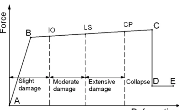
Structural members such as columns and beams are defined as nonlinear member frames. The nonlinear behavior of the structural members is represented by user-defined “lumped” plastic hinges and they are assigned to both ends of the columns and beams. Default or user-defined plastic hinges can be defined with the Sap2000 program. In Fig. 3, a typical force–deformation relationship of a plastic hinge is shown. It can be seen that points A, B, C, D and E can be used to express the behavior of the plastic hinge. Yield displacement is referred to by point B and point C refers to the maximum displacement capacity of members. Slight damage (SD), moderate damage (MD) and extensive damage (ED) regions can be determined after the calculation of IO, LS and CP deformation limits associated with the damage levels for the critical section of the ductile structural members. The coordinates of points A, B, C, D, and E and the deformation limits (IO, LS, CP) can be calculated using the cross-sectional properties, material qualities, longitudinal and trans-verse reinforcement details and axial load levels of structural members.
Fig. 3 Typical force–deforma-tion relaforce–deforma-tionship and deformaforce–deforma-tion limits for damage levels
Moment–curvature analyses were performed for each structural member by spreadsheet software provided by Ersoy and Ozcebe (2001) and the properties of user-defined plas-tic hinges were determined. In the moment–curvature analysis, confined and unconfined concrete behaviors are represented by the Modified Kent-Park model (Scott et al. 1982) and typical stress–strain curve with strain hardening is used for reinforcing steel behavior (Mander 1984).
In Fig. 3, point the B indicates the elastic force and displacement capacity of members and can be calculated by the Sap2000 program using the effective stiffness of members. In the study, the points C and D are taken equal to the CP deformation limit as the CP limit defines the limit of the behavior before collapsing according to TEC-2007 and 20% of flexural strength of the member was assigned as the point D in y axis shown in Fig. 3. Furthermore, the point E is assumed as 2 times of the point D in deformation (x axis). The effective stiffness of beams is considered as 0.4EI in the TEC-2007, and Eqs. (1a) and (1b) are recommended to calculate the effective stiffness of the columns depending on the axial load ratio. In Eqs. (1a) and (1b), N is axial load of column, Ac is column cross-sectional
area and fc is the compressive strength of concrete. Linear interpolation is recommended
for axial load ratio between 10 and 40%.
During the moment–curvature analysis, the damage limits of each member were also determined. The cross-sectional damage limits in the TEC-2007 at the critical sections of the structural members are given in Table 1 for the maximum concrete and steel strain lim-its. In Table 1, ρs and ρsm refer to the existing and required volumetric transverse
reinforce-ment ratios given in the TEC-2007.
The moment–curvature relationship at the critical sections of members is converted to a moment-rotation relationship. During the conversion of the moment-rotation relation-ship, the plastic hinge length was taken as half of the cross-section height in the considered direction as given in the TEC-2007.
Recent studies have indicated that due to low concrete strength and insufficient trans-verse reinforcement, shear effects should also be considered in addition to flexural responses to represent the actual behavior of the structures (Palanci et al. 2014, 2016). For this reason, brittle shear effects are also considered and shear hinges are introduced for the critical regions of the beams and columns. Ductility is not considered for the shear hinges because of brittle failure of concrete in shear. Thus, if the shear force in the member reaches its shear strength, the member fails immediately. The shear strength of a member (Vr) is calculated by Eq. (2) as suggested in Turkish standards TS-500 (2000). In the
equa-tion, bw and d represent width and the effective height of the cross-section, Asw and fy
rep-resent the cross-sectional area and the yield strength of shear reinforcement, s reprep-resents (1a) 0.4EI if N∕(Acfc)≤0.10
(1b) 0.8EI if N∕(Acfc)≥0.40
Table 1 Cross-sectional damage limits in the TEC-2007
Sectional damage Concrete strain (εc) Steel strain (εs)
Slight damage 0.0035 0.010
Moderate damage (MD) 0.0035 + 0.010(ρs/ρsm) ≤ 0.0135 0.040 Extensive damage (ED) 0.0040 + 0.014(ρs/ρsm) ≤ 0.0180 0.060
the distance between the transverse reinforcements and N/Ac is the ratio of axial load and
section area.
2.2 Capacity of the representative RC buildings
In order to obtain the capacity curves of the representative buildings, pushover analyses were performed and the base shear force and roof displacement relationship of the build-ings was determined. During the analyses, the buildbuild-ings were first subjected to gravity loads. Then, lateral force distribution was applied to each story level step by step and the capacity curves of the buildings were obtained. Lateral force distribution was obtained by multiplying each story weight and first modal shape amplitude at each story level. P–∆ effects were also considered in the analyses.
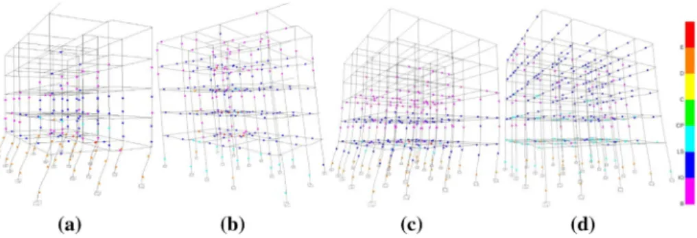
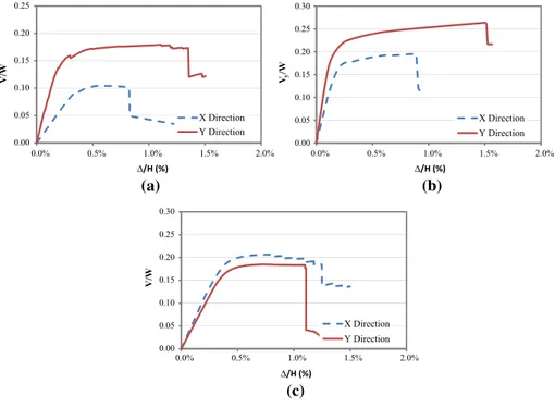
In Fig. 4, the plastic hinge formation of 5A and 5B buildings, at ultimate when the sig-nificant decay in lateral strength observed (see Fig. 5), is shown for readers to follow the discussions given in further paragraphs. In Fig. 5, the capacity curves of buildings 5A, 5B and 5C are plotted primarily for x and y directions. The vertical axis of the capacity curve represents the lateral strength ratio (Vy/W) obtained by proportion of the base shear force
and the seismic weight of the building. The lateral axis of the capacity curve represents the global drift ratio obtained by proportion of the roof displacement capacity and building height (Δ/H).
As seen in Fig. 5, the lateral strength ratio of building 5A is around 10% in x direction while it is 18% in y direction. The pushover analysis results showed that all the columns reached their moment capacity at the lower and upper ends at the base story in x direc-tion (Fig. 4a), but the lateral load capacity ratio of the building was calculated around 10% owing to lower moment capacities. However, the columns only reached their actual capac-ity at lower ends at the base story in y direction (Fig. 4b). This situation shows that the moment capacities of the columns are greater than those of beams (strong column-weak beam phenomenon). The maximum roof drift ratio of the building is obtained as 0.9 and 1.3% in x and y directions, respectively. Due to the insufficient confinement details of the structural members, the lower drift ratios are obtained for building 5A when compared with code-based constructed buildings.
(2) Vr= 0.182√fcbwd � 1+ 0.07N Ac � +Asw s fyd
Fig. 4 Plastic hinge formation of buildings 5A and 5B in both principal directions. a 5A-x direction. b 5A-y direction. c 5B-x direction. d 5B-y direction
The lateral strength ratio of building 5B is around 18 and 23% in x and y directions, respectively (see Fig. 5). When the floor plan of building 5B is inspected, it can be seen that the weak direction of the building is x direction. As well as in building 5A, the lower and upper ends of the columns reached their moment capacity in weak direction of building 5B (Fig. 4c). Furthermore, when the plastic hinge formation of principal y direction is checked (see Fig. 4d), it can be seen that only the lower ends of the columns are exceeded the yield level at the base story. In other words, the beams reached their moment capacity at the base story in y direction owing to the strong column-weak beam mechanism. In effect, this mechanism is preferred in design philosophy. However, lower moment values were obtained at the upper ends of the columns due to weak beams. Thus, this mechanism hindered the expectation of high capacity differences. The maxi-mum global drift ratio is obtained as 0.88 and 1.5% in x and y directions, respectively.
Figure 5 clearly indicates that the lateral strength and global drift ratio of building 5C is relatively close in x and y directions. It was observed that the lateral strength capacity ratios were around 20 and 18% while the drift ratios were around 1.3 and 1.1% in x and y directions, respectively.
As can be seen from Fig. 5, depending on the structural characteristics, different capacity curves are obtained from the representative buildings. The studies of Inel et al. (2008) and Akkar et al. (2005c) also stated the observation of considerable differences between the capacity curves of mid-rise RC buildings. The reasons for such differ-ences in the capacity curves were expressed and listed as the practice of constructing techniques, preliminary design, structural system characteristics, nonlinear behavior of structural mechanism and assumptions in the analysis models.
0.00 0.05 0.10 0.15 0.20 0.25 0.0% 0.5% 1.0% 1.5% 2.0% X Direction Y Direction ∆/H (%) ∆/H (%) ∆/H (%) V/ W 0.00 0.05 0.10 0.15 0.20 0.25 0.30 0.0% 0.5% 1.0% 1.5% 2.0% X Direction Y Direction Vy /W 0.00 0.05 0.10 0.15 0.20 0.25 0.30 0.0% 0.5% 1.0% 1.5% 2.0% X Direction Y Direction V/ W (a) (b) (c)
2.3 Equivalent SDOF systems of RC buildings
After the pushover analyses, the capacity curves of the representative buildings were idealized by bilinear curves considering the ATC-40 guideline and the EUROCODE-8. Spectral acceleration (Say) and hence displacement (Sdy) at yield was approximated by
the EUROCODE-8. The EUROCODE-8 approach was also utilized to equalize the areas under the actual curves and the idealized force–deformation curves. The ultimate displacement point (dp) was determined by the equal displacement approximation
sug-gested in the TEC-2007 and the EUROCODE-8. If the spectral displacement does not intersect the capacity curve then ultimate displacement of the buildings was attained when the significant decay in lateral strength was recorded. For this purpose, spread-sheet software which computes the dynamic properties of the building and performs iteration procedure to represent the bilinear behavior of the SDOF system was devel-oped by the authors. In Fig. 6, typical and idealized (bilinear) capacity curves (slope before yield K1 and post-yielding slope, K2) are shown.
The dynamic characteristics of the equivalent SDOF systems were then calculated in accordance with the ATC-40 guideline (modal mass coefficient (α1), modal participation
factor (Г1), natural periods (T1) and spectral quantities at yield and ultimate). In Table 2,
yield displacement of equivalent SDOF models (Δy) and the dynamic properties of each
Fig. 6 Typical pushover curve and bi-linearization
Table 2 Dynamic properties of equivalent SDOF models for representative RC buildings
Building model W (kN) H (m) Direction T1 (s) K2/K1 (%) α1 Г1 ∆y (m) Say (g)
5A 8295.06 14.80 X 1.16 4.240 0.873 1.286 0.037 0.110 Y 0.64 0.940 0.825 1.341 0.020 0.200 5B 11,587.75 14.70 X 0.63 1.264 0.893 1.253 0.020 0.200 Y 0.47 1.159 0.866 1.273 0.142 0.258 5C 7625.19 14.00 X 0.77 0.150 0.794 1.323 0.036 0.245 Y 0.86 1.520 0.794 1.324 0.041 0.225
representative building for x and y directions are given. In addition, the seismic weights (W) and building heights (H) of the representative RC buildings are provided.
3 Selection of ground motion record sets
In modern seismic codes, time history analysis is accepted as one of the analysis methods for design and/or performance evaluation (TEC-2007, FEMA-368, EUROCODE-8, ASCE 07-05, GB). According to the required conditions of these codes for time history analysis, code-compatible ground motion records can be used if the average response spectrum of the selected ground motion records is compatible with the design acceleration spectrum within a stated period range. In the present study, the TEC-2007 compatible ground motion records sets are used for nonlinear time history analysis. During the analyses equivalent SDOF models are used and hysteretic behavior is considered as elasto-plastic with post-yield hardening effects. In addition, the damping ratio of the buildings is taken equal to 5%. Ground motion records are selected from the European Strong Motion Database (Ambra-seys et al. 2004a). There are 2213 strong ground motion records available from 856 earth-quakes recorded at 691 different stations in the database (Ambraseys et al. 2004b).
3.1 Design acceleration spectrum and time history analysis procedure defined in the TEC‑2007
96% of Turkey’s land is located on different seismic zones (1st, 2nd, 3rd, 4th, and 5th degree seismic zones) according to the current seismic hazard zoning map prepared by the Ministry of Public Works and Settlement (http://www.depre m.gov.tr/en/categ ory/earth quake -zonin g-map-96531 ). For the seismic hazard map of Turkey, the seismic zones were determined by using acceleration zonation map that had been calculated with the prob-abilistic method. It assumes that for ordinary buildings the probability of exceedance of the expected maximum acceleration within a period of 50 years is 10%. Thus, earthquake zones of Turkey are classified as follows due to expected acceleration values. In accord-ance with the TEC-2007 the design ground acceleration is 0.40, 0.30, 0.20 and 0.10 g for the 1st, 2nd, 3rd and 4th degree seismic zones, respectively. The 5th degree seismic zone is accepted as a non-seismic zone and the design ground acceleration is zero for this zone.
In the TEC-2007, structures are designed by 5% damped elastic design spectrum that can be defined as an earthquake level that has a 10% probability of exceedance in 50 years for buildings with the building importance factor I = 1. The mathematical expression of this spectrum is given in Eq. 3. In Eq. 3, T1 is the first natural vibration period of building in
the direction of the earthquakes considered, TA and TB are the spectrum characteristic
peri-ods that depend on local soil classes defined in the TEC-2007, A0 defines effective ground
acceleration coefficient and I is the building importance factor (I = 1 for residential and office buildings). Four local soil classes are defined in the TEC-2007: Z1, Z2, Z3 and Z4. The local soil classes for TA and TB are given in Table 3. Elastic spectral accelerations are
calculated by multiplying A(T1) and gravity (g).
Earthquakes that cause serious loss of life and property in Turkey occur in the 1st degree seismic zone (Ilki and Celep 2012). In addition, the majority of Turkey’s existing building stock is located in cities in this seismic zone. Thus, in this study, the 1st seismic zone is considered. The effective ground acceleration coefficient A0, representing 1st degree
In Fig. 7, elastic spectral acceleration for local soil classes that would be used to determine seismic loads for the residential buildings, which are located in 1st degree seismic zone, are given.
In the TEC-2007, artificially generated, simulated or previously recorded ground motion records can be used to perform nonlinear time history analysis of buildings and building-like structures. Local site conditions should be appropriately considered in using recorded or simulated ground motions. At least three ground motion records should be used for time history analysis and the selected records should meet the fol-lowing criteria:
• The duration of strong ground motions should be greater than 5 times the natural period of the building and should be longer than 15 s.
• The average of zero-period spectral acceleration values of the selected ground motion records shall not be less than A0g for the buildings.
• The average of spectral acceleration values of the selected records shall not be less than 90% of the elastic spectral accelerations for the periods between 0.20T1 and 2.00T1
according to the first natural period of buildings T1 for considered analysis direction.
(3) A�T1 � = ⎡ ⎢ ⎢ ⎢ ⎣ � A0I �� 1+ 1.5T1 TA � 0 ≤ T1≤TA � A0I � 2.5 TA≤T1≤TB � A0I � 2.5 � TB T1 � T1≥TB ⎤ ⎥ ⎥ ⎥ ⎦ Table 3 Spectrum characteristic
periods for local soil classes Local soil TA (s) TB (s)
Soil Z1 0.10 0.30
Soil Z2 0.15 0.40
Soil Z3 0.15 0.60
Soil Z4 0.20 0.90
• The mean value of structural response from all of the analyses could be used if at least seven ground motion records are used; otherwise, the maximum value of structural response quantities should be used.
In addition to conditions described above, following additional criteria are considered during the obtaining of ground motion sets:
• In the TEC-2007, the lower limit of average spectral acceleration values of ground motion record sets is proposed as 90% of the elastic spectral acceleration, but the upper limit is not defined. In order to get more compatible results with the design spectra, the upper limit is also defined as 1.10. Accordingly, the average spectral acceleration value of ground motion record sets is limited between 0.90 and 1.10 of the elastic spectral acceleration for the periods between 0.20T1 and 2.00T1.
• The last criterion deals with the scaling factor used in scaling the amplitude of the original acceleration records. As known, the scaling factor plays a crucial role in the process and one prefers to keep modification of the original records to a minimum. In general, scale factors closer to unity are preferred and many ground motion experts rec-ommend a limit on the amount of scaling applied (Watson-Lamprey and Abrahamson 2006). Recommended limits on scaling typically range from factors of 2–4 (Bommer and Acevedo 2004). In this study, the scaling factor was adapted to 0.50–2.00.
3.2 Ground motion data sets
In this study, for each considered local soil class, the ground motion record sets included in three different earthquake groups that have 7, 11 and 15 number of ground motion compo-nents are used to perform nonlinear time history analysis. Five ground motion record sets are used in each earthquake group.
In order to obtain code-compatible ground motion record sets, initially, the following criteria of epicentral distance (R), magnitude (M) and peak ground acceleration (PGA) are used to obtain a catalogue from the European Strong Motion Database (Ambraseys et al. 2004a): R is in the range of 10–50 km; M is greater than 5.5; and PGA is 0.10 g or higher. Afterwards, ground motion record sets are obtained through record selection from the cata-logue. Considering the criteria, 542 horizontal components of 271 ground motion records are selected from the database for the catalogue.
These 542 horizontal components in the catalogue were grouped based on the local soil classes that they were recorded in. According to the EUROCODE-8 definition of local soil classes, there are 190 horizontal components of 95 ground motion records for soil class A; 236 horizontal components of 118 ground motion records for soil class B; and 116 hori-zontal components of 58 ground motion records for soil class C in the catalogue. It should be noted that there are very few ground motion records satisfying the abovementioned cri-teria about M, R and PGA in the database for soil class D and E. Thus, soil class D and E are ignored for the catalogue. Soil class Z1, Z2, and Z3 defined in the TEC-2007 are com-patible with soil class A, B and C defined in the EUROCODE-8, respectively. Hence, in order to obtain record sets for Soil class Z1, Z2 and Z3, ground motion records recorded on soil class A, B and C, are considered, respectively.
For each soil class of Z1, Z2 and Z3, 15 ground motion record sets are obtained, con-sidering that only those ground motion records are recorded in the matching soil class sites, i.e. on sites with the soil class A, B and C, respectively. Selection and scaling
ground motion records to match a given design spectrum can be formulated as an engi-neering optimization problem such that average square root of the sum of squares of the difference between the code-based response spectrum and average response spectrum of selected and scaled ground motions within a period range of interest (Naeim et al. 2004; Iervolino et al. 2008, 2010a). Required properties of ground motion records defined in seismic design codes can be considered as constraints of the optimization problems. When the selection and scaling problem defined and formulated as engineering optimi-zation problem, several methods can be used for the solution. In this study, a solution model based on heuristic harmony search algorithm (Geem et al. 2001) is used to obtain ground motion record sets. The detailed information on the ground motion selection procedure used in the present study can be found in Kayhan et al. (2011) and Kayhan (2016). It should be noted that all the 45 ground motion record sets are compatible with the TEC-2007 and are also satisfying all the constraints considered in this study. Appen-dix A provides the label of ground motion components and the corresponding scale fac-tors selected for all the ground motion record sets while Appendix B presents detailed information about the ground motion records.
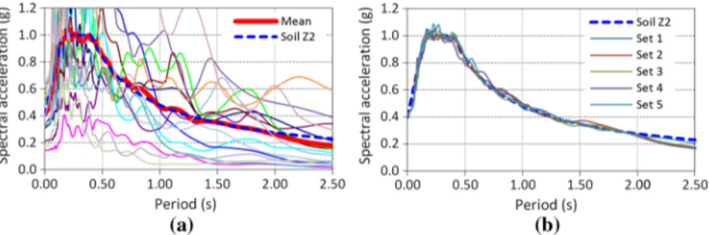
Figure 8 illustrates the representative examples for compatibility between the mean spectra of the ground motion record sets and the target spectra. Figure 8a shows the individual response spectra (thin continuous lines) and the mean spectrum (thick con-tinuous line) for Set 1 with 15 ground motion components, and the target spectrum for Soil Z2 (dashed line) can be shown. Figure 8b presents the mean spectra of five ground motion record sets with 15 ground motion components and the target spectrum for Soil Z2 can also be seen.
As can be seen from Appendix A, some horizontal components are in different ground motion record sets with different scale factors. For example, considering Soil Z1, “6333y” is selected in Set1 and Set2, “292y” is selected in Set4 and Set5 for the sets with 7 ground motion components and “369x” is selected in Set2, Set3 and Set4 for the sets with 11 ground motion components. However, it is not possible to say that some particular records are selected in many of the record sets. In addition, even if a ground motion component takes place in different record sets, it has different scale fac-tors in each record set. Thus, code-compatible record sets used in this study are ran-domly selected, and they can be accepted to be independent from each other. There is a possibility of selecting the same records in different code-compatible sets, because
Fig. 8 Representative examples for compatibility between mean spectra of the record sets and target tra defined in the TEC-2007. a The individual response spectra and mean spectrum for a set and target spec-trum. b The mean spectra of the five record sets and target spectrum
this situation is related with the number of ground motion records in a catalogue and the record numbers in a ground motion sets. If the number of records in a catalogue increases, this possibility may decrease and vice versa.
4 Evaluation of dynamic analysis results
4.1 The mean of maximum drift ratio demands for ground motion record sets
In this part of the present study, the drift ratio demands obtained using ground motion records sets are statistically evaluated. For this purpose, the maximum global drift ratios (Δmax/H) of the individual ground motions are determined from the nonlinear time history
analysis of the buildings. As mentioned before, in order to make seismic design or perfor-mance evaluation, the mean of structural responses can be used if at least seven ground motion records are used for the time history analysis according to modern seismic codes such as the TEC-2007, EUROCODE-8, FEMA-368 etc. In this study, record sets with 7, 11 and 15 ground motion records are used. Hence, the mean (µΔ/H) of the Δmax/H values of
records is calculated for each record set.
It can be seen from the Figs. 9, 10 and 11 that the µΔ/H values of buildings 5A, 5B and
5C, respectively are plotted according to the number of records, principal direction and soil class. It is worth reminding that for each number of records (7, 11 and 15) and soil class, five record sets are used. The µΔ/H values of each record set can be seen from the figures
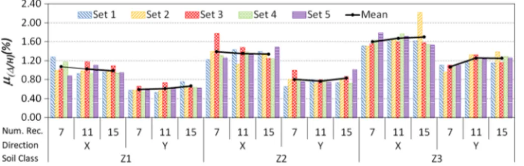
Fig. 9 µΔ/H values of the record sets calculated for building 5A
with distinct colors. In addition, the mean of five µΔ/H values are plotted for each number of
records in the set, soil class, and analysis direction.
The µΔ/H values of building 5A are given in Fig. 9 for each soil type. It can be seen from
the figure that the mean of maximum drift ratios are different, although all obtained records sets are compatible with the target spectrum for the considered soil type. The figure clearly indicates that the mean drift ratios are increasing on average from Z1 to Z3 soil class. For example, the µΔ/H values of the five sets with a number of seven records are 1.27, 0.99,
1.03, 1.18 and 0.88% for Z1 soil class and x direction. The average of these µΔ/H values of
the five sets is 1.07%. For Z2 and Z3 soil class, the averages of the µΔ/H values of the five
sets with seven records are 1.29 and 1.60% respectively. Vibration period of building 5A is
T1 = 1.16 s in x direction, As can be seen from Fig. 7, design spectral acceleration, A(T1),
is minimum for Z1 and maximum for Z3. According to TEC-2007, the average spectrum of the record sets should be compatible with corresponding target spectrum in considered period range (0.2T1–2.0T1). Thus, average spectrum has smaller value for the record sets
compatible with soil Z1 than the record sets compatible with soil Z2 and Z3 in this period range. In accordance with this situation, the mean drift ratio calculated for the record sets is the smallest for soil Z1 and the biggest for soil Z3. Furthermore, the increase in the number of records has no significant effect on the mean drift ratios of the record sets in any soil type. For example, the averages of the µΔ/H values (for x direction) of the five sets with
seven, eleven and fifteen records are 1.07, 1.02 and 0.99% respectively for Z1 soil class, and 1.39, 1.35 and 1.34% respectively for Z2 soil class.
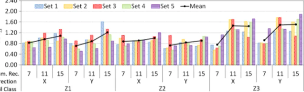
Figures 10 and 11 present the µΔ/H values calculated for buildings 5B and 5C,
respec-tively. Similar observations stated for building 5A are also valid for buildings 5B and 5C. Similarly, the µΔ/H values of code-compatible record sets are close to each other, the mean
drift ratios are increasing on average from Z1 to Z3 soil class and number of records has no apparent effect on the drift ratio demands.
The outcomes of this part clearly express that the mean of the maximum drift ratios of different record sets compatible with the same target response spectrum may be close to each other, but can show slight changes. Therefore, it can be said that the mean of the struc-tural responses considered for code-based seismic design and/or performance evaluation purposes will vary according to the ground motion records used. Reliability based approxi-mation may provide benefits to take account of the dispersion in structural responses. This approximation requires the detailed statistical evaluations of structural responses and their dispersions according to local soil classes or the number of records used for time history analyses. Thus, not only the central tendency but also dispersion of the structural responses is needed. For this reason, the dispersion of structural responses and the relationship Fig. 11 µΔ/H values of the record sets calculated for building 5C
between the dispersion and local soil classes and the number of records are investigated in the next section.
4.2 The dispersion of maximum drift ratio demands for ground motion record sets
In recent years, probability-based studies have become more prevalent (Lin 2008; Askan and Yucemen 2010; Mitseas et al. 2016; Kayhan and Demir 2016; Yamin et al. 2017) in the field of earthquake engineering. Probability-based seismic design or evaluation requires the knowledge of the probability distributions of seismic structural responses (e.g. maximum inter-story drift demand ratio) considered as random variables. In the cases in which the probability distributions of random variables cannot be precisely determined, the parame-ters of considered probability distribution are needed. For example, in addition to the mean (µ), there is also a need for a standard deviation (σ) which represents dispersion around the mean. One of the indicators of dispersion around the mean is the coefficient of variation (CoV), the ratio of the standard deviation to the mean. In order to evaluate the dispersion of
Δmax/H values in a record set around the mean of the same set µΔ/H, CoVΔ is calculated for
each ground motion record set.
In Fig. 12, CoVΔ distribution of building 5A is plotted for each soil class. In addition,
the mean of five CoVΔ values are plotted for each number of records in the set, soil class,
and analysis direction. As also shown by the figure, it can be said that dispersion of Δmax/H
values around the µΔ/H is quite high for each record set. The lowest and highest values were
determined to be 0.52 and 1.89, respectively. Obtained results imply that the dispersion is increasing with the increasing number of ground motions in the record sets even if they are compatible with the same target design spectrum.
CoVΔ distributions of building 5B and 5C are separately illustrated in Figs. 13 and 14.
In some record sets, CoVΔ values are even higher than 2.0, especially for Z3 soil class and
similar to building 5A, the dispersion of 5B and 5C buildings is also high for all considered soil classes and record sets. Dispersion of drift ratios increases with the increasing num-ber of records in the record sets. CoVΔ values get remarkably higher, especially for the Z3
classes and considered buildings.
It is a known fact that seismic codes especially focus on matching between target response spectrum and mean response spectrum of a record set within a certain period range, but they do not consider the compatibility between individual records and target response spectrum. In this case, for any period value in the considered period range, the scatter of spectral acceleration of the individual records (Sa) in the record set around the
mean (μSa) of the same record set cannot be controlled and high variations can be observed.
Accordingly, the variations in ∆max/H (or any structural response considered) values of
individual records around the μ∆/H of the record set can be high. For example, if the Set1 of
Z2 soil class shown in Fig. 8 is considered, it can be seen that Sa values of 15 records range
between 0.181 and 1.641 g at the period of 0.47 s that of the natural period of building 5B in principal y direction. At the period 0.47 s, spectral acceleration values of target spectrum and mean of record set are 0.879 and 0.898 g, respectively. It can be said that the mean of records sets and target spectrum spectral acceleration values have very good agreement, but dispersion of Sa values is very high. CoVSa value for this period is 0.57.
In Fig. 15, CoVSa values of the record sets are illustrated according to the local soil
types and the number of records in the set for each building used in this study. As known, five record sets are considered for each soil class. The individual points in the figure rep-resent CoVSa values calculated for each of the record sets. Continuous and dashed lines are
Fig. 13 CoVΔ values of the record sets calculated for building 5B
Fig. 14 CoVΔ values of the record sets calculated for building 5C
plotted to point the means of CoVSa values for x and y directions. It can be understood from
the figure that the variations in Sa(T) values are also very high.
In general, Fig. 15 implies that CoVSa values of ground motion sets are also higher than
0.4. If the continuous or dashed lines corresponding to the means of CoVSa values are
fol-lowed, it is possible to say that CoVSa values are also increasing with an increasing number
of ground motion records. For example, considering building 5A and soil Z1, the means of
CoVSa are 0.65, 0.83, and 0.93 for x direction and 0.60, 0.67, and 0.72 for y direction, for
the record sets with 7, 11 and 15 records, respectively. Besides, considering the building 5C, CoVSa values are increasing with an increasing number of records in a set for all the
soil types considered. It can be said that a similar situation is observed in the building 5B except for the record sets that have 15 records for the Z2 soil class.
The results summarized in Figs. 12, 13 and 14 imply that the application of the current code-compatible requirements given in the TEC-2007 similar to the modern seismic codes around the world may cause high dispersions in terms of structural responses. A similar observation was reported by Iervolino et al. (2010b). Katsanos et al. (2010) also high-lighted similar findings by using the Eurocode-8 compatible ground motion record sets.
In addition to the requirements given in the seismic codes, the other factor that causes high dispersion in structural responses may be the limited number of ground motion records in record catalogues. Ground motion record sets are selected from the pre-selected record catalogues by considering some specific criteria. If a catalogue with smaller number of real ground motion records is used, the variation of spectral acceleration values in the sets may larger. As mentioned earlier, the record sets used in this study for the soil classes Z1, Z2 and Z3 are selected by using a catalogue of 190, 236, 116 record components, respectively. According to Fig. 15, the CoVSa values of the record sets compatible with the
soil Z3, which are obtained by selecting from the catalogue with lower number of record components, are higher. If you have a catalogue with limited number of real ground motion records with different compatibility with design spectrum, the use of the larger number of ground motion records for the sets may further increase of the variation of spectral acceler-ation values in the sets. If lower number of records is preferred, relatively more compatible records with design spectrum may be selected for a set. Thus, dispersion of spectral accel-eration values may be lower. If the number of records is increased, relatively less compat-ible records with design spectrum may be added to set. In this case, dispersion of spectral acceleration values may increase. If the high dispersion of spectral acceleration values is the reason of the high dispersion of drift ratio demands, the dispersion of the drift ratio demands may further increase with the larger number of ground motions in the record sets.
4.3 One‑way analysis of variance (ANOVA)
The results provided in Figs. 9, 10 and 11 indicate that the mean drift demands calculated for different ground motion record sets compatible with the same design spectrum are close to each other. Thus, it can be said that the mean drift demand calculated for a building is a random variable which depends on the record sets used for the time history analysis. In order to evaluate the differences between the mean drift demands of five ground motion record sets for each building and principal analysis direction, one-way analysis of variance (ANOVA) is used. Each local soil type and the number of ground motion record in a set are also separately considered for one-way ANOVA. One-way ANOVA is used to determine whether there is any statistically significant difference between the means of three or more independent samples using the F-test (Gamst et al. 2008).
The null hypothesis for one-way ANOVA refers to that the means of all populations are equal for c independent samples that have normally distributed k size members [Eq. (4)]. In order to test the null hypothesis, the source of two variations: the variation between sample means (SSA) and the variation within samples (SSW) should be calculated. Mathematical expressions of sum of squares among (SSA) and sum of squares within (SSW) are given in Eqs. (5) and (6). Total variation is the sum of SSA and SSW. In the equations, c is the num-ber of samples, kj and μj define the member size and the mean of sample j, respectively, and
μall is the mean of all samples, while Xij refers to the ith member of sample j.
The degrees of freedom between samples are calculated by c − 1 while those within samples are calculated by n − c. To calculate the degrees of freedom within samples, n, the sum of member sizes of all samples is needed. Afterwards, two variances, the mean squares between samples (MSA) and within samples (MSW) are calculated by using Eqs. (7) and (8). Lastly, the F statistic, simply a ratio of two variances, is determined by taking the ratios of MSA and MSW.
F value is mostly illustrated by using a tabular format shown in Table 4. Finally, F value is compared with F-critical value. F-critical value is upper critical value of the F distri-bution with the significance level (α) and degrees of freedom within samples (n − c) and between samples (c − 1). Significance level is used to represent the value of an F-critical value having cumulative probability of (1 − α) and mostly taken equal to 5%. If the F value is smaller than the F-critical value, null hypothesis (H0) is accepted.
In this study, five different record sets are used for each considered local soil class and number of ground motion records in a set. Thus, c = 5. However, n, the sum of member (4) H0∶𝜇1= 𝜇2= 𝜇3= ⋯ = 𝜇c (5) SSA= c ∑ j=1 kj(𝜇j− 𝜇all)2 (6) SSW= c ∑ j=1 k ∑ i=1 ( Xij− 𝜇j )2 (7) MSA= SSA c− 1 (8) MSW= SSW n− c
Table 4 Typical representation of one-way ANOVA table Source of variation Sum of squares (SS) Degrees of
freedom (df) MS (Variance) Computed F
Among samples SSA c − 1 MSA F =MSWMSA
Within samples SSW n − c MSW
sizes of all samples, varies with the number of ground motions in a record set. For the record sets with 7, 11 and 15 ground motion records, n is 35, 55 and 75, respectively. Thus, considering α = 0.05, the F-critical value for the record sets with 7, 11 and 15 groups are 2.690, 2.557 and 2.503, respectively. The F values calculated for each building, principle direction, local soil class and the number of ground motion records in a set are plotted in Fig. 16.
The figure demonstrates that the highest F value is calculated as 0.576 and the corre-sponding F-critical value is 2.690. Thus, H0 is accepted. In other words, the drift demands
obtained by using five ground motion record sets that are compatible with the same design spectrum are drawn from the populations with an equal mean at the 95% confidence level. The lower value of F indicates that the effect of variability within samples (MSW) due to the random causes on the total variability is larger than the effect of variability between samples due to the differences between the mean of samples. Thus, the differences between the mean of samples are accepted statistically insignificant considering the results of one-way ANOVA. According to the F-values given in Fig. 16 and the corresponding F-critical values, H0 is also accepted for the other buildings, local soil types and the number ground
motion records sets examined in this study.
One-way ANOVA results have demonstrated that the mean drift demands of different ground motion record sets which are compatible with a particular design spectrum can be treated as they are random samples of the same populations. In this case, some conclusions can be drawn about the distribution of populations by using relevant drift demands.
In order to make a seismic design or evaluation, mean structural responses can be used according to modern seismic codes. However, it should be noted that randomly changing structural responses may be obtained for each ground motion record sets compatible with the considered design spectrum. Thus, it would be useful to obtain data on the distribu-tion of mean structural responses. It can be useful to use an interval of mean structural responses for a particular confidence level. Furthermore, dispersion of structural responses should also be taken into consideration for a reliability based seismic design or evaluation.
4.4 Sampling distributions of mean drift demand ratios
Sampling distribution can be defined as the distribution of a statistic for all possible sam-ples taken from the same population. It is derived from a random sample of size n. Thus,
0.00 0.20 0.40 0.60 0.80 Z1 Z2 Z3 Z1 Z2 Z3 Z1 Z2 Z3 Z1 Z2 Z3 Z1 Z2 Z3 Z1 Z2 Z3 X Y X Y X Y 5A 5B 5C F value s
Sets with 7 records Sets with 11 records Sets with 15 records
Direction Building Soil Class
the sampling distribution of a statistic depends on the sample size and the sampling proce-dure. Sampling distributions can be characterized by two important statistics: sample mean (m) and the sample variance Var(m). The sampling distribution of the mean, namely the probability distribution of mean (m), represents the variability of sample means m around the population mean μ.
In this study, considering the prescribed degree of confidence within which the popu-lation parameters μ lie, interval estimates of drift demand ratios are calculated. For the population parameter μ, the probability statement of the interval estimates can be given as follows in Eq. 9:
In Eq. 9, l and u donate the lower and upper confidence limits, respectively. l and u depend on the numerical value of the sample mean m for a particular sample. The 1 − α is defined as the confidence coefficient. The interval (l, u) refers to the 100(1 − α)% confi-dence interval for the parameter μ. The quantity 100(1 − α)% is the conficonfi-dence level of the interval.
For a random sample of n observations taken from a normally distributed population with the mean μ and the variance σ2, the value of the sample mean m is calculated by using
the values of the random variables in the sample. In this case, m is also a random variable. It is expected that the sample mean m is centered about the population mean μ, but its dis-persion decreases when the sample size increases (Eq. 10).
Considering a large sample of size n from a population with the mean μ and the vari-ance σ2, the Central Limit Theorem specifies that sample distribution is normal even if the
population does not come from a normal distribution and the sample mean m will be equal to population mean (μ) and variance can be calculated by the proportion of population vari-ance and sample size (σ2/n). If the sample size is small, the Student’s t distribution can be
used to calculate the confidence intervals of population mean μ. For a random sample of size n and 100(1 − α)% confidence interval, interval estimates of μ are given by Eq. 11. In Eq. 11, tα/2,n−1 is the upper 100α/2 percentage point of the t distribution with n − 1 degrees
of freedom and s∕√n is the standard error of sample means.
In practice, confidence intervals are mostly taken as 90 or 95% confidence level. In this study, 90% confidence level is used for representative calculation. It should be noted that one can use any confidence level and corresponding confidence limits for a specific seismic design and/or an assessment study.
The 90% confidence intervals (l, u) for the mean of the populations of drift demand ratios (μΔ/H) are calculated for each building, analysis direction, local soil class and the
number of records in a set. As mentioned before, five different ground motion sets are used for each local soil class and considered number of ground motion records in a set. Hence, n is taken equal to 5 and the corresponding tα/2,n−1 is calculated as 2.13 for the corresponding
confidence interval of the population means.
The central tendency of sample means of drift demand ratios ( ̄m ) are given in Fig. 17. As shown in the figure, ̄m values vary with the building and analysis directions considered, (9) P(l ≤ 𝜇 ≤ u) = 1 − 𝛼 0 < 𝛼 < 1 (10) E[m] = 𝜇 and Var(m) =𝜎 2 n (11) m− t𝛼∕2,n−1√s n ≤ 𝜇 ≤m+ t𝛼∕2,n−1√s n
and increase if the soil class changes from Z1 to Z3. For example, for the building 5A and the ground motion record sets with 7 records, the value of ̄m is 1.18% for soil Z1, 1.38% for soil Z2 and 1.64% for soil Z3 considering X direction. For the same building and the record sets, the value of ̄m is 0.69, 0.93 and 1.14% in Y direction for the Z1, Z2 and Z3 soils, respectively. In Fig. 17, the values of ̄m vary randomly with the number of ground motion records in record sets, but they are relatively close to each other. For example, for the building 5B and soil class Z1, the value of ̄m in X direction is 0.62, 0.55 and 0.61%, in Y direction it is 0.47, 0.40 and 0.45% for the record sets with 7, 11 and 15 ground motion records, respectively. It can be said that there is no significant effect of the number of ground motion record sets in record sets on ̄m values, Table 5 displays the 90% confidence interval (l, u) of the mean drift demand ratios of the populations (μΔ/H) together with the
relevant ̄m values.
According to the Table 5, for the building 5A, soil Z1 and direction x, the confidence interval of μΔ/H is (0.922, 1.220%) for the sets with 7 records, (0.917, 1.131%) for the sets
with 11 records and (0.926, 1.048%) for the sets with 15 records. These confidence inter-vals indicate that if different ground motion record sets compatible with design spectrum for the soil class Z1 were used for the nonlinear time history analysis of the building 5A in direction x, the calculated mean drift demands (μΔ/H) of the records sets would be between
the abovementioned lower and upper confidence limits with a 90% probability.
5 Conclusions
In this study, the global drift ratio demands obtained by nonlinear time history analysis using different code-compatible real ground motion record sets are statistically evaluated and the effect of the number of ground motion record sets is investigated. Three mid-rise RC buildings, representing the existing mid-rise buildings in Turkey, are selected and the drift ratio demands calculated for the selected buildings are evaluated in terms of mean and dispersion. The ground motion record sets compatible with the design spectra defined for local soil classes in TEC-2007 are considered. For each local soil class, five different ground motion record sets with 7, 11 and 15 ground motion records are used. The key observations and findings of this study are briefly summarized as follows:
1. The dispersion of the maximum drift ratio demands in a record set is quite high and as a result of investigations, it is suspected that the limited number of records in the cata-logues, where the ground motion records are selected, could lead to high variability in drift ratio demands. In this study only one strong ground motion database (Ambraseys et al. 2004a, b) is used. Nowadays, many databases including a large number of strong ground motion records are also available such as Engineering Strong Motion (Luzi et al. 2016) and PEER Strong Motion Database (Ancheta et al. 2014). Using one or more of these databases this variability can be lowered. Moreover, results demonstrated that the variations of Z3 soil which have lower number of ground motion records in the catalogue is specifically higher. It is also possible to say that the dispersion of drift ratio demands increase proportional to the number of ground motion records in a record set. This result is valid for a wide range of vibration periods between 0.46 and 1.16 s which represent the first-mode dominated mid-rise RC buildings.
2. Observations have also shown that there is not a particular effect of the number of ground motion records (record set which have more than seven records) on the mean drift ratio demands. Thus, use of at least seven records seems adequate and practical for the design and evaluation practices.
3. Results obviously showed the possibility of obtaining distinct mean drift ratio demands for different record sets which have same number of records (e.g. 5 different record sets which have 7 records or higher) although they are compatible with the same design spectrum.
4. In order to explain variability of mean drift ratio demands for different ground motion record sets, one-way ANOVA is used. Although there is a clear variability among the record sets, ANOVA results demonstrated that mean drift ratio demands of different Table 5 90% confidence intervals (l, u) for μΔ/H (%)
Record number Soil class Direction Building 5A Building 5B Building 5C
̄ m l u m̄ l u m̄ l u 7 Z1 X 1.071 0.922 1.220 0.533 0.498 0.567 0.697 0.608 0.787 Y 0.594 0.553 0.635 0.408 0.372 0.444 0.772 0.717 0.827 Z2 X 1.392 1.179 1.605 0.699 0.631 0.766 1.033 0.846 1.220 Y 0.805 0.685 0.925 0.452 0.414 0.489 1.133 0.866 1.400 Z3 X 1.600 1.486 1.715 1.001 0.928 1.075 1.390 1.263 1.517 Y 1.067 1.005 1.129 0.760 0.677 0.844 1.310 1.289 1.330 11 Z1 X 1.024 0.917 1.131 0.553 0.490 0.615 0.711 0.650 0.772 Y 0.613 0.539 0.687 0.398 0.353 0.444 0.763 0.713 0.813 Z2 X 1.350 1.218 1.483 0.657 0.619 0.696 0.981 0.925 1.038 Y 0.766 0.733 0.800 0.473 0.440 0.506 1.049 0.957 1.141 Z3 X 1.672 1.608 1.736 1.145 1.096 1.194 1.556 1.454 1.658 Y 1.256 1.191 1.321 0.903 0.831 0.974 1.547 1.477 1.617 15 Z1 X 0.987 0.926 1.048 0.586 0.555 0.618 0.848 0.757 0.939 Y 0.667 0.617 0.716 0.412 0.374 0.450 0.836 0.749 0.924 Z2 X 1.339 1.238 1.440 0.719 0.628 0.811 1.029 0.870 1.188 Y 0.830 0.717 0.944 0.492 0.457 0.527 1.092 0.967 1.218 Z3 X 1.700 1.422 1.979 1.131 1.064 1.198 1.542 1.424 1.659 Y 1.250 1.159 1.341 0.907 0.833 0.981 1.518 1.373 1.663