An application of capacitated lot-sizing model in petroleum sector

(1)

AN APPLICATION OF CAPACITATED LOT-SIZING

MODEL IN PETROLEUM SECTOR

A THESIS

SUBMITTED TO THE DEPARTMENT OF INDUSTRIAL ENGINEERING

AND THE INSTITUTE OF ENGINEERING AND SCIENCES OF BILKENT UNIVERSITY

IN PARTIAL FULFILLMENT OF THE REQUIREMENTS FOR THE DEGREE OF

MASTER OF SCIENCE

by

Nuri Barış Nurlu February 2006

(2)

I certify that I have read this thesis and that in my opinion it is fully adequate, in scope and in quality, as a thesis for the degree of Master of Science.

____________________________________ Assoc. Prof. Osman Oğuz (Principal Advisor)

____________________________________ Prof. Dr. Nesim K. Erkip

____________________________________ Asst. Prof. Bahar Yetiş Kara

Approved for the Institute of Engineering and Sciences

____________________________________ Prof. Dr. Mehmet Baray

(3)

ABSTRACT

AN APPLICATION OF CAPACITATED LOT-SIZING MODEL IN PETROLEUM SECTOR

Nuri Barış Nurlu M.S. in Industrial Engineering Supervisor: Assoc. Prof. Osman Oğuz

February 2006

In this thesis, we study capacitated lot-sizing problem with special feature, applicable to the petroleum refinery sector. In our model, the end-products should be stored in item-specific and capacitated storage tanks during pre-determined lead-time. Our aim is to find the optimum production schedule resulting minimum total cost whilst satisfying customer demand. To solve this problem in a reasonable amount of time, we propose a branch-and-cut algorithm. We perform experiments based on the data gathered from Turkish Petroleum Refineries Corporation. In order to evaluate our algorithm, we compare the results of our algorithm and the solution results of the optimization software.

Keywords: Lot-sizing, branch-and-cut, mixed-integer-programming, petroleum sector, refinery

(4)

ÖZET

KAPASİTELENDİRİLMİŞ ÖBEK BÜYÜKLÜĞÜ MODELİNİN PETROL ENDÜSTRİSİ ÜZERİNE UYGULAMASI

Nuri Barış Nurlu

Endüstri Mühendisliği, Yüksek Lisans Tez Yöneticisi: Doç. Dr. Osman Oğuz

Şubat 2006

Bu tezde, petrol rafinerilerinde uygulama bulabilecek özel nitelikteki kapasitelendirilmiş öbek-büyüklüğü problemi üzerinde çalıştık. Modelimizde bitmiş ürünler, ürün spesifik ve kapasitesi sınırlı saklama tanklarında önceden belirlenmiş önsüre zamanınca beklemek durumdadırlar. Amacımız, müşteri talebini karşılarken en düşük maliyete ulaşabileceğimiz en iyi üretim çizelgesini bulabilmekti. Bu problemi kabul edilebilir bir süre içerisinde çözüme ulaştırmak için dal-ve-kesi algoritması önerdik. Türkiye Petrol Rafinerileri Anonim Şirketi’nden elde ettiğimiz verilerle hesapsal deneylemeler uyguladık. Algoritmamızı değerlendirmek amacıyla, algoritma sonuçlarımızla eniyileme yazılımımızın sonuçlarını karşılaştırdık.

Anahtar sözcükler: Öbek büyüklüğü, dal-ve-kesi, karışık tam sayılı programlama, petrol endüstrisi, rafineri

(5)

To Cemile and Başak...

(6)

To The One...

(7)

ACKNOWLEDGMENT

I would like to express my sincere appreciation to Assoc. Prof. Osman Oğuz for his guidance, attention, support, interest and patience during my study. Studying under his supervision is one of the most valuable experiences during this thesis study for me.

I am indebted to Prof. Nesim K. Erkip and Asst. Prof. Bahar Yetiş Kara for accepting to read and review this thesis, and for their effort, time, kindness and support.

During my graduate studies, I am also involved in BOTAŞ BTC Project Directorate. I would like to thank Dr. Mr. Kaan Tunçok, my line-manager; Mr. Sarper Kaptan, Completions Manager; Mr. Adem Yılmaz, Deputy Project Manager (Human Resources) and Miss. Pınar Güralp, my colleague for their support, patience and assistance.

I would like to express my appreciation to Bob Daniel, from Dash Optimization, for providing me XPRESS-MP licenses. Also I would like to thank Assoc. Prof Oya Ekin Karaşan for providing me the license dongle of XPRESS-MP.

I would like to thank Burakhan Yalçın and Utku Koç for their endless friendship and support. I am also indebted for all Industrial Engineering Department staff.

(8)

LIST OF FIGURES

3-1a: Gap between lower bound and best solution when we solve MIP problem without applying (l, S) cuts…...……….30

3-1b: Gap between lower bound and best solution when we solve MIP problem with applying (l, S) cuts …..………..31

3-2a: Search tree of problem solved without branch-and-cut………...32

(11)

LIST OF TABLES

4-1: Computational Results for η=20, τ=20...37

4-2: Computational Results for η=20, τ=30.. ...38

4-5a: Statistics of the computational experiments... ...40

4-5b: Statistics of the computational experiments... ...41

4-6: Summary of Computational Experiments...42

4-7: Statistics of Computational Experiments...43

A1-1a: Computational Results for η=5, τ=5...48

A1-1b: Computational Results for η=5, τ=10...49

A1-1c: Computational Results for η=5, τ=20...49

A1-1d: Computational Results for η=5, τ=30...50

(12)

List of Tables

(13)

List of Tables

A2-1a: Distributions of Parameters………60

A2-1b: Distributions of Parameters………61

A2-1c: Distributions of Parameters………62

A2-1d: Distributions of Parameters………63

A2-1e: Distributions of Parameters………64

A2-1f: Distributions of Parameters……….65

(14)

C h a p t e r 1

Introduction

Since late 90s, Supply Chain Planning (SCP) has been one of the most popular planning strategies in global business environment. SCP studies primarily focus on production planning, pricing, scheduling, and warehouse-planning, and aim to achieve cost minimization, profit maximization, process improvement and increase in sales. As Chen and Chu (2003) indicate, advanced supply chain planning is the process of balancing materials and planning resources to satisfy customer demands while achieving the business goal for reducing costs. Thus, fulfilling the demand with minimum costs possible should be the core of business to create a high quality supply chain flow.

One of the subareas of production planning is the lot sizing problem, which can be defined as the objective to satisfy customer demand whilst minimizing the total production, setup and inventory holding costs. As the output of lot-sizing problem, we obtain the optimum production

(15)

Chapter 1 - Introduction

schedule which gives us the answers of questions of when and how much/many we ought to produce, with minimum total cost possible.

In this thesis, the lot sizing problem with a special feature introduced and the solution procedure of this problem is discussed. In our model, the end products should be kept in a warehouse for a certain pre-determined duration for resting purpose. The end-products should be kept in storage tanks in order to rest the petroleum, in petroleum companies like Turkish Petroleum Refineries Corporation (TÜPRAŞ). Similar strategy –for different aim– is also applied in dairy product companies, like Danone. After fermentation and packaging operations, the end-products should be stored in warehouse for refrigerating and making them durable to the last day. Moreover, the total warehouse capacity is divided into subareas depending on the number of end-items. This situation occurs especially in petroleum industry in which each end-item should be stored in unique storage tanks. As a consequence, the problem that we will study throughout the thesis involves the production planning problem occurring in the petroleum refinery sector.

Aside from certain uncapacitated versions, lot-sizing problem is NP-hard. Especially when the size of the problem grows, the model cannot be solved optimally within an acceptable time. Thus, it is required to generate an alternative solution technique, to solve the problem in a relatively short period of time, without significantly deviating from the optimum solution. In our thesis, we applied branch-and-cut algorithm to our model to reach the optimum solution in reasonable amount of time.

(16)

Chapter 1 - Introduction

In computational experiments of this thesis, test data is generated based upon the data gathered from TÜPRAŞ and run under XPRESS-MP optimization software in order to interpret how the constructed technique behaves in different data sets.

In Chapter 2, a comprehensive survey in literature about the research on lot-sizing theory is presented. In Chapter 3, the problem and the corresponding constructed model are introduced. The solution technique and its steps are discussed in the same chapter. In Chapter 4, the computational experiments are reported. Conclusion and remarks for future studies are given in Chapter 5.

(17)

C h a p t e r 2

Literature Review

The lot-sizing problem, as a subclass of the production planning problem, aims to satisfy customer demand without violating the capacity restrictions imposed on production resources — whilst minimizing the total production, setup and inventory holding costs (see Salomon and Kuik (1993)). Most of the research on lot-sizing problems focuses on generating new algorithms and heuristic approaches to find the optimal solutions of various kinds of lot-sizing problems. Below we review some previous work that is related to the subject of this thesis.

As indicated above, the main purpose of the lot sizing problems is to satisfy customer demand. However, in certain cases, the customer demand cannot be fulfilled due to the capacity restrictions. In such a situation, company should choose one of the three possible solutions as a company strategy regarding its long term costs and profits. First approach is lost sales, in which the company simply refuses the customer’s demand. Backlogging (back ordering) is the second approach where

(18)

Chapter 2 - Literature Review

customer is offered to wait for at least one more period to buy the desired product. The last approach is called as outsourcing. Here, the company supplies the similar product from another company (probably its competitor) and sells it to its customer immediately.

The first lot-sizing problem published in the literature is the single period, single item, and uncapacitated lot-sizing problem with deterministic demand. Harris (1913) named this problem as Economic

Order Quantity (EOQ). Though the paper was published in 1913, the

subject still attracts attention of researchers due to its importance in production planning theory. Wagner and Whitin (1958) published another classical and pioneering paper, which provides a dynamic programming and network approach to lot sizing problems.

2.1 Classifications of Lot-Sizing Problems

Before going further into the studies previously made in the lot-sizing literature, it is necessary to introduce some lot-sizing terminology and mention classifications of the problem. Lot-sizing problems can be classified either as capacitated or uncapacitated, depending on the restrictions on the resources such as labor, machinery or time. The capacity restrictions might be set either as hard constraint or soft constraint. In the first case, the restrictions cannot be violated by any situation. On the other hand, in soft constraint case, the restriction might be violated with some penalty cost depending on the significance of the restriction. As we shall see in the following sections, the capacity

(19)

limitation is one of the most important factors and determines the difficulty of the problems.

Secondly, the pattern of customer demand might be deterministic or stochastic. Deterministic demand is used by the companies, which start production after taking the orders. However in the literature, even if the real situation is stochastic, deterministic demand is assumed to simplify the problem.

Furthermore, models may or may not include the setup cost depending on the problem structure. Similarly, setup time is another factor to be considered while model constructing. Moreover, allowing backorder/lost sales/outsourcing, and varying the number of machines in production facility are some other types appeared in lot-sizing models mentioned in Staggemeir et. al. (2001), and Katok et al. (1998). In Federgruen and Meissner (2005), multiple items for different demands sharing the same resources are also studied.

The cost functions of the lot-sizing problems —the objective functions to be minimized— are non-decreasing in the amount produced or stored, usually linear, fixed-charge or general concave functions; Hoesel, Romeijn, Morales and Wagelmans (2002).

The general capacitated lot-sizing problem is proved to be NP-hard according to Aghezzaf and Landeghem (2002).

(20)

According to Katok, Lewis and Harrison (1998), the difficulty of production planning problems arise from (i) cumulative capacity usage, (ii) ratio of setup times to processing times and (iii) ratio of setup costs to inventory costs. In the same study it is stated that, there is a trade-off between the quality of the solution and computational effort required to solve the problem.

Salomon and Kuik (1993) indicate that when setup times are non-zero, the problem is NP-Hard, even for the single level single resource problems. Likewise, multi-level and capacitated problem is NP-hard, since it is a direct generalization of the capacitated lot-sizing problem with non-stationary capacities (see Hoesel, Romeijn, Morales and Wagelmans (2002)).

In Florian, Lenstra and Kan (1980) and Hoesel et. al. (2002), it is proved that a production planning problem is NP-hard, even when it has equal demand structure and zero inventory costs, where

(i) no setup costs and no capacity limits exist, but the cost function is arbitrary,

(ii) no setup costs and capacity limits are arbitrary and cost function is concave, or

(iii) convex cost function and unit setup cost exist, with no capacity limits.

(21)

In Wolsey (1998), it is shown that the single item capacitated lot-sizing problem reduces to the knapsack problem, which means that the lot-sizing is NP-hard.

2.2 Solution Approaches

In his study on modern heuristic techniques, Reeves (1993) states that: “Developing algorithms, which are computationally successful at solving combinatorial optimization problems, is an art.”

Salomon and Kuik (1993) and Katok, Lewis and Harrison (1998) divide the solution approaches into two, as optimization (effort to reach the optimum within a reasonable time) and heuristic approaches (effort to find the “good” solution in a “small” time period). Katok et. al (1998) states that optimization approaches are valuable since they generate good lower bounds to be used in heuristic techniques. On the other hand, Chen and Chu (2003) state that there are four different classes to solve lot-sizing problems: (i) Integer Programming Approaches (ii) Decomposition Methods, (iii) Local Search Techniques, (iv) Lagrangean Relaxation Techniques.

(22)

2.2.1 Integer Programming Approaches

The Linear Programming (LP) Relaxation of Mixed Integer

Programming (MIP) of the problem, also known as the LP Based

solution technique, forms the first class of the solution techniques for lot-sizing problems. Available methods relax the capacity and/or balance constraints to bring an ease to the problem. Nevertheless, this technique lowers the quality, in terms of optimality of the solution. We will review some papers focusing on Branch-and-Bound, Branch-and-Price and Branch-and-Cut for the Integer Programming (IP) Approaches.

In terms of data set, Branch-and-Bound approach, which is one of the most popular methods to solve lot-sizing problem, is fast for the small problems (see Clark (2003)). Unfortunately, it is concluded that as the problem size grows, the combinations, which should be followed by the procedure, explode exponentially.

In Degraeve and Jans (2003-1), Branch-and-Price algorithm, which is a new formulation of Dantzig-Wolfe decomposition technique, is introduced for the lot-sizing problems. In this algorithm, initially an upper-bound is gathered, then, in order to find a good lower-bound of IP, column generation technique is applied. Finally, simplex and subgradient optimization is utilized, and column generation and branch-and-bound are combined.

(23)

Branch-and-Cut algorithm, on the other hand, is a branch-and-bound algorithm in which cutting planes are generated throughout the Branch-and-Bound tree. Strong valid inequalities and reformulations often form the basis of branch-and-cut algorithms and create good models for complicated problems (see Atamtürk and Munoz (2004)).

Degreave and Jans (2003-1) indicates, regular capacitated lot-sizing problem with setup times usually has a large integrality gap. Many researchers are devoted to finding better formulations with a smaller gap. Degreave and Jans (2003-1) extend their model with valid inequalities, which are generally known as (l, S) inequalities. Adding these cutting planes leads to a formulation which describes the convex hull for the lot-sizing polytope. On the other hand, whilst focusing on cut-and-branch techniques, Miller, Nemhauser and Savelsbergh (2000) also mention the (l, S)-type valid inequalities, which generate the convex hull for each item. It is also defined that the “path inequalities” which generalize the (l, S) inequalities, for more general lot-sizing and other fixed-charge network flow problems. It is also indicated that in solving multi-item models, the (l, S) inequalities have often been the most effective known class.

According to Miller et al (2000), there are two palpable merits of using (l, S) inequalities. The first is that the algorithm –if it has time to terminate– finds a provably optimal solution. The second is that a feasible solution is found if one exists, this characteristic is not shared by the many heuristic methods (such as proposed by Trigeiro et al. (1989)).

(24)

A disadvantage of such an optimization approach is that it can require much time and memory, possibly an indefinite amount of both.

2.2.2 Decomposition Methods

The second class is the decomposition method, in which certain parts of the problem are decomposed and solved disjointedly. For instance, during the application of decomposition technique to the lot-sizing problem within a multi-level structure, it ignores the multi-level structure and solves the sequence of single-level ones.

Degraeve and Jans (2003-1) have a study on reformulation of the decomposition of lot-sizing problems. They separate the setup and production decisions, and solve the problem. The solution yields the same lower bound as branch-and-price algorithm, which leads us to the conclusion that branch-and-price algorithm is computationally obedient and competitive, with respect to other approaches. Similarly, Degraeve and Jans (2003-2) aim to improve the lower bounds of the capacitated lot-sizing problem using Dantzig-Wolfe decomposition and Lagrangean Relaxation.

2.2.3 Local Search Techniques

The third approach to solve lot-sizing problems is the meta-heuristics, which consist of local search techniques such as Simulated Annealing,

(25)

Tabu Search, Genetic Algorithm and Evolutionary Strategies (see Staggemeier and Clark (2001)). These techniques generally aim to find near-optimal solutions in relatively small amount of time.

Kuik and Salomon (1990) and Salomon and Kuik (1993) study on the disadvantages of Simulated Annealing and Tabu Search. First of all, the performance of algorithms turns out to be strongly dependent upon a large number of interrelated factors such as the problem structure and choice of internal parameters. Furthermore it is unknown how far a solution given by this approach differs from optimality due to computation of lower bound. Hertz, Taillard and de Werra (1995) indicate that these methods generally obtain reasonable solutions to a number of complex combinatorial optimization problems when standard procedures like decomposition or relaxation techniques fail.

In Gopalakrishnan, Ding, Bourjolly and Mohan (2001), it is concluded that the sequencing (the sequence in which the final-products should be produced) and lot sizing problems are interrelated decisions. Gopalakrishnan et. al (2001) claims using meta-heuristics to be practical since they are easily extended to handle simulations like scheduling on multiple machines.

Staggemeier et. al. (2002) test their problem by the Genetic Algorithm and they indicate that allocation and sequence of products become the most important feature of the algorithm in the effort to escape from the local optima. Also, in terms of average deviation from the optimum

(26)

Reeves (1993) mentions one additional local search technique called

artificial neural networks. The system is represented by networks and

when it is used to solve IP problems, it copies the biological neuron systems in terms of methodology. It is useful to encode many optimization problems (like scheduling), but it does not attract considerable attention of researchers’ since it needs so much effort to setup the system.

2.2.4 Lagrangean Relaxation Techniques

Finally, the Lagrangean-based approaches use the Branch-and-Bound strategy followed by smoothing procedures to eliminate the infeasibilities. Lagrangean Relaxation is also used to find strong lower bounds for heuristic techniques.

In general, the problems are classified as easy in terms of their complexity, if some of their constraints such as capacity restrictions are excluded. Lagrangean based approaches concentrate on eliminating such difficult constraint sets (Reeves (1993)). On the other hand, Lagrangean dual problem, which is used to construct the Lagrangean solution, is the problem of minimizing the piecewise linear convex non-differentiable function (for minimization problems) (Wolsey (1998)).

(27)

One of the most classical papers in lot-sizing studies belongs to Trigeiro, Thomas and McClain (1989). The results of the study have become a benchmark for many studies, after it was published. They focus on the effects of setup time on general problem structure. Trigeiro et. al conclude that problems with setup times are really difficult, and it is a grave error to state that setup time is a simple extension of a setup cost.

2.3 Other Studies

Beside the solution techniques reviewed in the previous section, Walukiewicz (1991) states that in future, the hybrid algorithms, which combine certain algorithms or heuristics, will gain popularity. Hybrid algorithms try to solve the trade-off between solution quality and computational effort (Clark (2003)). He also mentions two methods to obtain a hybrid:

(i) searching for the best proportion by which you can factor setup times into unit production times; and

(ii) carrying out a local search on the first stages of binary setup variables.

(28)

Another concern in lot-sizing theory is lead time, which is the period of time between the initiation of any process of production and the completion of that process. Lead-time issue is rarely integrated into lot-sizing studies though it is one of the core effects of real supply chain. This is explained with fixed lead-times which are generally negligible (Stadtler (2003)). On the other hand, Clark and Armentano (1995) integrate lead-time into inventory variables to find the echelon stock policies in model’s structure. Moreover, in certain cases, lead-time is added to the balance constraints, as a function of a specific item (Chen and Chu (2003)).

In the lot-sizing literature, similar to other MIP problems, the models are commonly solved either by CPLEX, GAMS or XPRESS-MP, which are the major optimization softwares available in the marketplace. In our study, XPRESS-MP is preferred for its comparatively better Graphical User Interface (GUI) and ease of accessibility.

(29)

C h a p t e r 3

Problem and the Solution Approach

In this chapter, initially, the problem statement and corresponding mixed integer programming model will be presented including the explanations of the objective function and constraints. Subsequently, the proposed solution approach and the algorithm will be provided. With the intention of providing detailed explanation of the proposed algorithm, a small example and illustration will be presented to show the efficiency of the solution technique.

3.1 Problem Statement

According to The Investigation Process Research Library

(http://www.iprr.org), refinery is defined as any process plant in which flammable or combustible liquids are produced from crude petroleum, including areas on the same site where the resulting products are blended,

(30)

Chapter 3 – Problem and the Solution Approach

A refinery uses styrene, butadiene and aromatic oil beside crude oil in order to produce asphalt, LPG (liquid petroleum gas), diesel fuel, fuel oil, gasoline, kerosene, lubricating oils, paraffin wax, tar, extract etc. as end-products.

The main operations in the oil refinery are atmospheric distillation unit (distills crude oil into fractions), vacuum distillation unit (further distills residual bottoms after atmospheric distillation), naphtha hydrotreater unit (desulfurizes naphtha from atmospheric distillation), catalytic reformer unit (uses hydrogen to break long chain hydrocarbons into lighter elements that are added to the distiller feedstock), distillate hydrotreater unit (desulfurizes distillate (diesel) after atmospheric distillation), fluid catalytic converter unit, dimerization unit, isomerization unit, gas storage units for propane and similar gaseous fuels at pressure sufficient to maintain in liquid form, and storage tanks for crude oil and finished products, with some sort of vapor enclosure and surrounded by an earth berm to contain spills .

In our problem, we will focus on the production planning problem of a refinery company, which has number of refinery plants to produce aforementioned end-products. Each plant has its own capacity restrictions.

The demand is received by the company, so it is indifferent which refinery plant makes the production. We assume that if the demand

(31)

cannot be satisfied due to the capacity restrictions, then lost sales strategy will be applied.

Since the end-products are in liquid form, the storage tanks are assigned specifically to each product. So the maximum inventory for each item is limited. Besides, each end-product should be stored in the warehouse during some pre-determined duration, depending on product type, for resting. This duration is assumed to be constant in our model, however in real case; there exist an upper and lower bounds for resting periods.

Our problem also covers setup and production times. The setups are not allowed to be carried over from one period to another. Thus if one end-item is produced at time t, and it will be still produced at time t+1, we still consider extra setup time and cost for this end-item.

Our aim is to satisfy customer demand with minimum inventory holding, production, setup, and lost-sales costs.

3.2 Problem Formulation

In the mathematical model of the aforementioned production planning problem and throughout the thesis, we will use the following notation:

(32)

Sets

η

number of end-products

τ

number of time periods

R number of refineries of the company

Subscripts

i subscript for end-products, i ∈ [1, η] r subscript for refinery plants, r ∈ [1, R] t subscript for time periods, t ∈ [1, τ]

li required lead-time (resting time) to store item i after

production

Decision Variables

xirt production amount for item i at time t at refinery r

yirt    = otherwise 1, item for at time refinery at occurs setup no if , 0 r t i

Iirt inventory of item i at the and of the period t at refinery r

(33)

Parameters

cit cost of produce 1 unit of item i in period t

sit setup cost of item i, at time t (for all refineries r)

hit inventory holding cost for item i in period t

pit lost-sales cost of item i in period t

dit demand of item i in period t

Cit production capacity for item i in period t, for each refinery r

fir 1 if item i is produced at refinery r, 0 otherwise

Fr capacity of refinery r, for each time period t

Sir warehouse storage limit for item i at refinery r

ui required time to produce 1-unit of item i

vi total required time to set up item i for all time periods t

and for all refineries r

T total available time for production and setup for each time period for all end-products

We assume that setup time (

v

i) is only dependent on i, but not refinery r,

since one of our main assumptions is utilities (machines) in the refineries are similar in all refineries. So there is no need to add refinery index to setup time. Moreover, we do not add refinery index r to production capacity (

C

it), since

C

it is generally a big number indicating to combine

production (

x

irt) and setup (

y

irt) variables. The restriction on refinery

(34)

Mathematical Model

The mathematical formulation of the capacitated lot-sizing problem in accordance with the above mentioned notation and under the assumptions explained is as following:

.

)

1 (

)

(

min

t

s

y

s

I

h

x

c

D

p

z

i t r irt it irt it irt it it it

∑∑

∑













+

=

[ ]

1 ,

,

[ ]

1 ,

(

2 )

)

(

_, _,

−

_, _, ₁

+

_, _,

∈

η

∈

τ

−

=

d

∑

x

₋

I

₋ ₋

I

₋

i

t

D

r l t r i l t r i l t r i it it _i _i _i

[ ]

1 ,

,

[

1 ,

]

,

[ ]

1 ,

(

3 )

∈

η

∈

τ

≤

C

y

i

r

R

t

x

_irt _it _irt

[

1 ,

]

,

[ ]

1 ,

(

4 )

∈

τ

≤

∑

f

x

F

_r

r

R

t

i irt ir

[ ]

1 ,

,

[

1 ,

]

,

[ ]

1 ,

(

5 )

, , ,

≤

S

i

∈

η

r

∈

R

t

∈

τ

I

_i _r _t _i _r

(35)

[

1 ,

]

,

[ ]

1 ,

(

6 )

)

(

+

≤

∈

τ

∑

u

x

v

y

T

r

R

t

i irt i irt i

[ ]

[

]

[ ]

[

]

[ ]

1 ,

,

[

1 ,

]

,

[ ]

1 ,

(9)

0 (8)

1,

t

,

1 ,

,

1 }

1 ,

0 {

(7)

1,

t

,

1 ,

,

1

0 ,

,

,k i i,r irt irt irt irt

l

k

R

r

i

I

R

r

i

y

R

r

i

D

I

x

∈

=

∈

≥

η

τ

η

τ

η

Explanations of the Objective Function and Constraints

Objective function (1) minimizes total production, inventory holding, setup and lost sales costs during all time periods for all items and all refinery plants of the company.

Constraint set (2) is called as balance constraint. Lost-sale amount is equal to the difference between the demand and production amounts, regarding the on-hand inventory and inventory left to subsequent time period. Note that since there is an obligation to rest the end-products in storage tanks, required and related lead-time is subtracted from the indices of production and inventory variables. However, it may be

(36)

possible to define a new demand variable

d

it

’

representing the demand of

item i after

l

i, and eliminate subscript

l

i.

Constraint set (3) combines production variable and setup variable. If production occurred, so does setup.

C

_it gives upper bound for production.

Constraint set (4) is refinery-capacity constraint. Each item is produced at some refineries. However, maximum amount of items that each refinery can produce is limited for each time unit. Constraint (4) satisfies this rule.

Constraint set (5) limits the storage capacity of warehouse for each final product. In some industries –as beer-production industry–, the tanks can be cleaned and cleared before refueling items, in order to store different end-products. In our case, we assume that storage tanks are assigned specifically to each end-item.

T

is defined as the total available production and setup time within each time period. In our experiments, we assume each time period is one calendar day. Consequently,

T

is total available time for setup and production. Constraint set (6) mathematically represents that the total time spent for production and setup cannot exceed

T

.

(7) forces production, inventory and lost-sale variables to be nonnegative –since petroleum is liquid– and (8) obliges setup variable to be binary. Finally, (9) brings initial conditions that before lead-time, there is no

(37)

inventory for any item. If the system is currently working, then

I

irk can

easily be updated to a constant.

In all cases, the required lead-time

l

i is always less then total number of

time periods τ (0 <

l

i < τ , ∀i).

3.3 Solution Technique

In order to solve the capacitated lot-sizing problem introduced in the previous section, we apply branch-and-cut algorithm. The branch-and-cut algorithm is a branch-and-bound algorithm in which cutting planes are generated throughout the branch-and-bound tree (see Wolsey (1998)).

Many combinatorial optimization problems can be solved by branch-and-cut methods, which are exact algorithms consisting of a combination of a cutting plane method with a branch-and-bound algorithm. In general, branch-and-bound algorithms, which use divide and conquer approach, are precede cutting plane methods. Cutting plane methods improve the solution quality of the relaxed problems.

During the branching operation in the branch-and-bound algorithm, this philosophy adds cuts to the nodes. However, a trade-off of the branch-and-cut technique is the following: if many cuts are added at each node, then the re-optimization may be much slower than before. In addition, keeping all the information in the tree is significantly more difficult.

(38)

Thus we prefer to add cuts to the first 30-levels of the search tree. In other words, we will add cuts only to the nodes, which are generated at most 30 branching operations from the initial node of the search tree.

In branch-and-bound technique, the problem to be solved at each node is obtained just by adding bounds. However, in branch-and-cut, a cut pool is used, where all the cuts are stored. In addition to keep the bounds and a good basis in the node list, it is also necessary to indicate which constraints are needed to reconstruct the formulation at the given node. So indicators to the appropriate constraints in the cut pool are reserved.

The step-by-step description of the algorithm used in the thesis is as follows:

1. Set incumbent solution zinc = + INFINITY. Let L be the set of

active nodes. If L is empty, then STOP.

2. Preprocess the initial problem (in accordance with the preprocessing routine of XPRESS-MP).

3. If L is empty then STOP, zinc is the optimum solution; otherwise

select and delete node k from L (in accordance with the node selection routine of XPRESS-MP).

4. Solve the LP Relaxation of the problem. If all variables are integral, then STOP, solution is optimum. Else go to 5.

(39)

5. Set zinc be the objective value of LP, preprocess the problem.

6. Search for violated cutting planes, configurable to generate cuts to execute one or several cut generation iterations per node. If found, add them to the relaxation and return 4.

7. If found objective value is less then zinc, then go to 3. Otherwise,

if solution is integral feasible, update zinc and go to 3. If not

integral go to 6.

By default, XPRESS-MP does not apply any preprocessing routine to the problem introduced. In Step 2, we allow XPRESS-MP to do preprocessing.

In Step 6, we perform two operations: Firstly, XPRESS-MP only generates Gomory cuts at the top node by default. We use this option to generate cuts at the first 30-levels of the search tree. Secondly, we add (l, S) cuts.

It is vital to note that, if the problem is feasible, then there exists an integral feasible solution. At worse case, none of the demands is satisfied and all are lost –in which we reach maximum objective function value possible– .

The (l, S) inequalities, which are valid and proved to be useful cuts (see Chapter 2 for detail). These inequalities can be described as following:

(40)

potential production (

C

it

y

irt) in periods 1 to k (k

∈

[1,

τ

]) must at least

equal to the total demand in periods 1 to k in order not to pay penalty cost (

p

it). First of all, we assume that lost-sale is not allowed. Let

Q

ikm be the

total demand between time periods k and m for end-item i (m

∈

[1,

τ

],

(i

∈

[1,

η

]). Then mathematically,

[ ]

1 ,

,

[ ]

1 ,

(

10 )

∈

η

∈

τ

=

∑

=

m

k

i

d

Q

m k t it ikm Thus,

[ ]

1 ,

,

[

1 ,

]

,

[ ]

1 ,

(

11 )

)

,

min(

₁ 1

τ

η

∈

≥

∑

=

k

R

r

i

Q

y

C

x

_i _k k t irt it irt is valid.

For each time period

k

and each subset of periods

G

of 1 to

k

, the (l, S) inequality –expanded demand constraint– is (in accordance with the Pochet and Wolsey (1994)’s proof),

[ ]

1 ,

,

[ ]

1 ,

,

[

1 ,

]

(

12 ).

1 1 1

R

r

k

i

Q

y

Q

x

_i _k k G t t irt itk k G t t irt

+

∑

≥

∈

∑

∉ = ∈ =

τ

η

(41)

However, since our model allows lost-sale, we rewrite (12) as

[ ]

1 ,

,

[ ]

1 ,

,

[

1 ,

]

(

13 ).

1 1 1 1

R

r

k

i

y

Q

x

Q

D

k G t t irt itk k G t t irt k i k w iw

∈

−

≥

∑

∉ = ∈ = =

τ

η

The inequality (12) indicates that actual production (

x

irt) in periods

included in

G

plus maximum potential production

Q

itk

y

irt in the

remaining periods (those not in

G

) must at least equal to the total demand in periods 1 to

k

in order not to have infeasibilities. Note that in period

t

at most

Q

itk production is required to meet demand up to period

k

. On the other hand, in inequality (13), lost sale variable is redefined. If left-hand-side of the inequality (13) is negative (that is if demand is less then the sum of production up to k and production capacity after k), then according to (7), total lost-sale between time periods 1 and k will be 0. Pochet and Wolsey (1994) prove that when inequality (11) holds, then (12) is the most violated inequality for a given value of

k

.

3.4 Example and Illustration

In order to demonstrate how our algorithm works, we will present an instance from a small example. Assume that in our Mixed Integer Programming

τ

=

k

= 5,

η

= 2, R = 2. By definition,

G

will be the each

(42)

subset of 1 to

k

. Thus, the expanded demand constraints for this problem can be represented as follows:

)

5 (

)

(

)

4 (

)

(

)

3 (

)

(

)

2 (

)

(

)

1 (

)

(

115 114 113 112 111 115 5 1 1 115 155 114 113 112 111 5 1 115 1 115 155 114 145 113 112 111 115 5 1 1 115 155 114 145 113 135 112 111 5 1 115 1 115 155 114 145 113 135 112 125 111 115 5 1 1

e

x

Q

D

e

y

Q

x

Q

D

e

y

Q

y

Q

x

Q

D

e

y

Q

y

Q

y

Q

x

Q

D

e

y

Q

y

Q

y

Q

y

Q

x

Q

D

w w w w w w w w w w

+

−

≥

+

−

≥

+

−

≥

+

−

≥

+

−

≥

∑

= = = = =

The inequalities (e1) to (e5) are generated for i = 1, r = 1; thus as a consequence we should produce 15 more inequalities to complete all required cuts.

In (e1), the subset

G

is {1}. Similarly, the other subsets

G

for inequalities (e2) to (e4) are {1, 2}, {1, 2, 3}, {1, 2, 3, 4} and {1, 2, 3, 4, 5}.

(43)

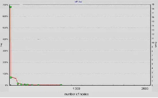
In order to illustrate the optimization process of our algorithm, we will demonstrate two graphics. In Figure 3-1a and 3-1b, we graphically present the gaps (percentage of difference between best solution and lower bound) occurred between the best solution value found at time t and the maximum lower bound found at the same time. In Figure 3-1a, which belongs to the experiment without applying our algorithm (XPRESS-MP uses its own cuts); we realize that in the first seconds, the gap decreases from 700% to 20%. The gap reaches 0 in 14 seconds with passing 2527 nodes. On the other hand in Figure 3-1b, the gap dramatically reaches 0 within the first second.

Figure 3-1a Gap (percentage of difference) between lower bound and best solution when we solve MIP problem without applying (l, S) cuts

(44)

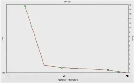
Figure 3-1b Gap (percentage of difference) between lower bound and best solution when we solve MIP problem with applying (l, S) cuts (with

respect to number of nodes).

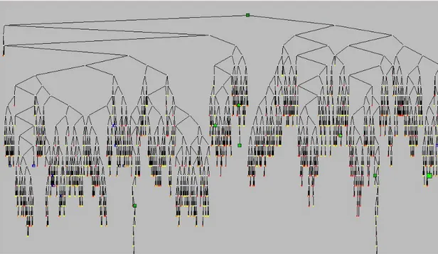
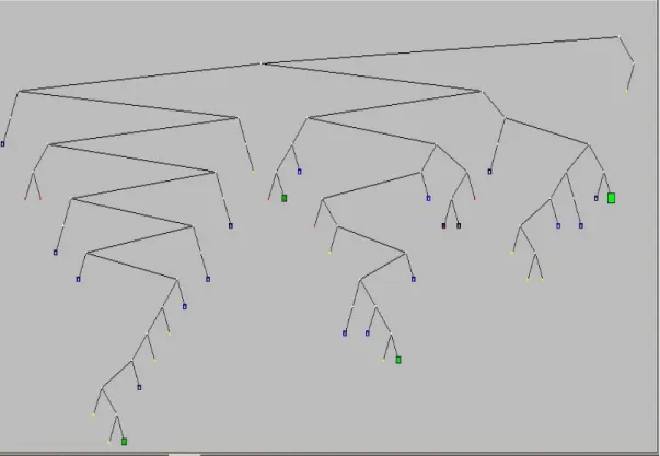
The search tree shown in Figure 3-2a belongs to the problem solved without applying branch-and-cut algorithm. Here we have 2527 nodes and search is completed within 13,6 seconds. In Figure 3-2b, the search tree belongs to the branch-and-cut solution. Here we have 84 nodes and the search is completed within 0,9 seconds.

(45)

(46)

(47)

C h a p t e r 4

Computational Experiments

In this chapter, we will report the results of the computational experiments of the algorithm proposed in Chapter 3. We will first present the experimental settings and then the results of the experiments. Following, we discuss and analyze the computational results.

4.1 Settings

The test data is gathered from the official web site of Turkish Petroleum Refineries Corporation (TÜPRAŞ). The demand and capacity data is converted into daily bases since TÜPRAŞ publishes annual data. Then we generate similar demand and capacity data allowing deviating ±10% from the gathered data for our different experiment sets. However, the cost data (cost parameters for production, setup, lost sales and inventory holding) is generated randomly, since this information is not provided by TÜPRAŞ.

(48)

Chapter 4 – Computational Experiments

The li values are selected randomly between 1 and 3. By generating the

random data, the penalty cost for lost sales is selected to be much more than other costs. Whilst selecting the range for setup cost, we considered that –in most cases– setup cost should take values between penalty cost (

p

it), and production costs (

c

it) for producing 1 lot.

Our algorithm was implemented in XPRESS Mosel and executed on a computer equipped with Intel Celeron 1.7 GHz processor, 256 MB RAM and Microsoft Windows 2000 SP4.

In our problem, there exist three sets as we defined in Chapter 3: number of end-items (η), number of production periods (τ) and number of refineries (R). In our experiments we test our algorithm for the cases of when η ∈{5, 10, 15, 20, 30}, τ∈{5, 10, 20, 30} and R∈{1, 2, 4}. This means, for instance η=10, τ=20, R=4 is one set of experiment which means there exists 10 end-products, produced in 4 refineries during 20 time periods. For each combination, we apply 5 replications. So we have total of 5 . 4 . 3 . 5 = 300 instances generated. We give 1-hour (3600 sec) to run the original program (without branch-and-cut) and 5-minutes (300 sec) to run branch-and-cut algorithm. We again remind that in all cases,

the required lead-time

l

i is always less then total number of time periods τ

(49)

4.2 Computational Results

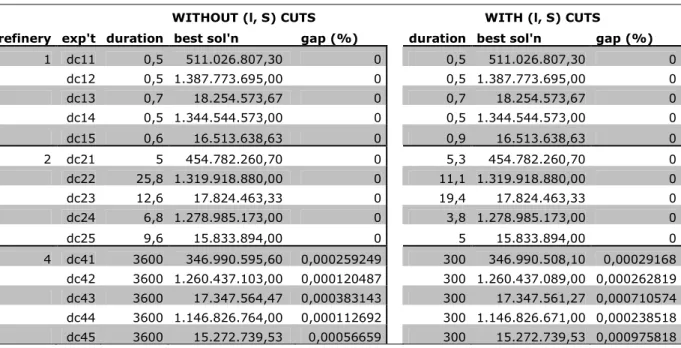
The computational results of the experiments are shown in the following pages. Each table represents the instances of specific η-τ pair. Under refinery column, we indicate the R value. For each case, we replicate 5 experiments (see exp’t column). The WITHOUT (l, S) CUTS columns represent the results of the experiments when we do not apply our algorithm. In this situation, our optimization software adds its own cuts and performs its branching operations. On the other hand, WITH (l, S) CUTS columns represent the results of the experiments when we apply our branch-and-cut algorithm. The duration values are CPU-times measured in seconds and gap represents the gap between lower bound and best solution value in percentage. In this chapter, we will only illustrate four tables. In Appendix-1, we will present all 20 tables of the experiment results.

In Table 4-1, we present the computational results for the case 20-items and 20-time periods. Here, we realize that when there exist single or double refinery in the system, the problem is trivial. On the other hand, in 4-refinery cases, our algorithm reaches better solutions in 4 experiments out of 5.

(50)

WITHOUT (l, S) CUTS WITH (l, S) CUTS

refinery exp't duration best sol'n gap (%) duration best sol'n gap (%) 1 dc11 0,5 511.026.807,30 0 0,5 511.026.807,30 0 dc12 0,5 1.387.773.695,00 0 0,5 1.387.773.695,00 0 dc13 0,7 18.254.573,67 0 0,7 18.254.573,67 0 dc14 0,5 1.344.544.573,00 0 0,5 1.344.544.573,00 0 dc15 0,6 16.513.638,63 0 0,9 16.513.638,63 0 2 dc21 5 454.782.260,70 0 5,3 454.782.260,70 0 dc22 25,8 1.319.918.880,00 0 11,1 1.319.918.880,00 0 dc23 12,6 17.824.463,33 0 19,4 17.824.463,33 0 dc24 6,8 1.278.985.173,00 0 3,8 1.278.985.173,00 0 dc25 9,6 15.833.894,00 0 5 15.833.894,00 0 4 dc41 3600 346.990.595,60 0,000259249 300 346.990.508,10 0,00029168 dc42 3600 1.260.437.103,00 0,000120487 300 1.260.437.089,00 0,000262819 dc43 3600 17.347.564,47 0,000383143 300 17.347.561,27 0,000710574 dc44 3600 1.146.826.764,00 0,000112692 300 1.146.826.671,00 0,000238518 dc45 3600 15.272.739,53 0,00056659 300 15.272.739,53 0,000975818

Table 4-1 Computational Results for

η

=20,

τ

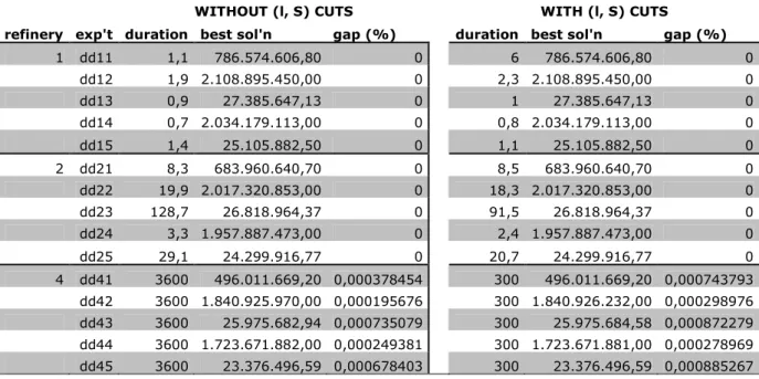
=20,

In Table 4-2, 20-items, 30-time periods case is tabulated. Here, again single and double refinery models are trivial. In 4-refinery cases, we again reach better solution in 4 cases out of 5.

(51)

refinery exp't duration best sol'n gap (%) duration best sol'n gap (%) 1 dd11 1,1 786.574.606,80 0 6 786.574.606,80 0 dd12 1,9 2.108.895.450,00 0 2,3 2.108.895.450,00 0 dd13 0,9 27.385.647,13 0 1 27.385.647,13 0 dd14 0,7 2.034.179.113,00 0 0,8 2.034.179.113,00 0 dd15 1,4 25.105.882,50 0 1,1 25.105.882,50 0 2 dd21 8,3 683.960.640,70 0 8,5 683.960.640,70 0 dd22 19,9 2.017.320.853,00 0 18,3 2.017.320.853,00 0 dd23 128,7 26.818.964,37 0 91,5 26.818.964,37 0 dd24 3,3 1.957.887.473,00 0 2,4 1.957.887.473,00 0 dd25 29,1 24.299.916,77 0 20,7 24.299.916,77 0 4 dd41 3600 496.011.669,20 0,000378454 300 496.011.669,20 0,000743793 dd42 3600 1.840.925.970,00 0,000195676 300 1.840.926.232,00 0,000298976 dd43 3600 25.975.682,94 0,000735079 300 25.975.684,58 0,000872279 dd44 3600 1.723.671.882,00 0,000249381 300 1.723.671.881,00 0,000278969 dd45 3600 23.376.496,59 0,000678403 300 23.376.496,59 0,000885267

η

=20,

τ

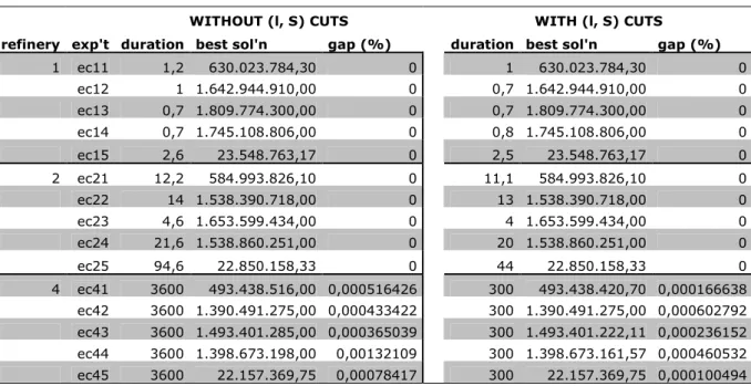
=30

In 30-items, 20-time periods case (see Table 4-3) and 30-items, 30-time periods case (see Table 4-4), we observe similar results. In first case, 5 (out of 5) and in second case, 4 (out of 5) results are better than the solutions of the experiments that we do not apply our algorithm. In all cases, we allow to run experiments with our algorithm 300 seconds and without our algorithm 3600 seconds. So even if our algorithm reaches worse solutions in 300 seconds, it is significantly different the results of non-algorithm in 3600 seconds.

(52)

refinery exp't duration best sol'n gap (%) duration best sol'n gap (%) 1 ec11 1,2 630.023.784,30 0 1 630.023.784,30 0 ec12 1 1.642.944.910,00 0 0,7 1.642.944.910,00 0 ec13 0,7 1.809.774.300,00 0 0,7 1.809.774.300,00 0 ec14 0,7 1.745.108.806,00 0 0,8 1.745.108.806,00 0 ec15 2,6 23.548.763,17 0 2,5 23.548.763,17 0 2 ec21 12,2 584.993.826,10 0 11,1 584.993.826,10 0 ec22 14 1.538.390.718,00 0 13 1.538.390.718,00 0 ec23 4,6 1.653.599.434,00 0 4 1.653.599.434,00 0 ec24 21,6 1.538.860.251,00 0 20 1.538.860.251,00 0 ec25 94,6 22.850.158,33 0 44 22.850.158,33 0 4 ec41 3600 493.438.516,00 0,000516426 300 493.438.420,70 0,000166638 ec42 3600 1.390.491.275,00 0,000433422 300 1.390.491.275,00 0,000602792 ec43 3600 1.493.401.285,00 0,000365039 300 1.493.401.222,11 0,000236152 ec44 3600 1.398.673.198,00 0,00132109 300 1.398.673.161,57 0,000460532 ec45 3600 22.157.369,75 0,00078417 300 22.157.369,75 0,000100494

η

=30,

τ

=20

refinery exp't duration best sol'n gap (%) duration best sol'n gap (%) 1 ed11 1,1 980.947.801,30 0 1 980.947.801,30 0 ed12 1,3 2.626.700.398,00 0 1,1 2.626.700.398,00 0 ed13 1,1 2.761.191.015,00 0 1,1 2.761.191.015,00 0 ed14 1,2 2.871.287.461,00 0 1,1 2.871.287.461,00 0 ed15 3,3 35.956.220,58 0 1,1 35.956.220,58 0 2 ed21 1,3 883.262.428,40 0 1,1 883.262.428,40 0 ed22 13,3 2.502.518.067,00 0 11 2.502.518.067,00 0 ed23 197,3 2.668.271.006,00 0 67,3 2.668.271.006,00 0 ed24 10,5 2.742.101.775,00 0 5,1 2.742.101.775,00 0 ed25 12,8 35.050.735,00 0 11,3 35.050.735,00 0 4 ed41 3600 732.483.934,80 0,000292533 300 732.483.834,44 0,000905531 ed42 3600 2.309.743.795,00 0,000617352 300 2.309.743.689,13 0,000593759 ed43 3600 2.315.188.088,00 0,00087874 300 2.315.188.007,01 0,000520516 ed44 3600 2.499.453.434,00 0,00179219 300 2.499.453.434,00 0,000202116 ed45 3600 33.952.760,00 0,000756007 300 33.952.768,10 0,000693635

(53)

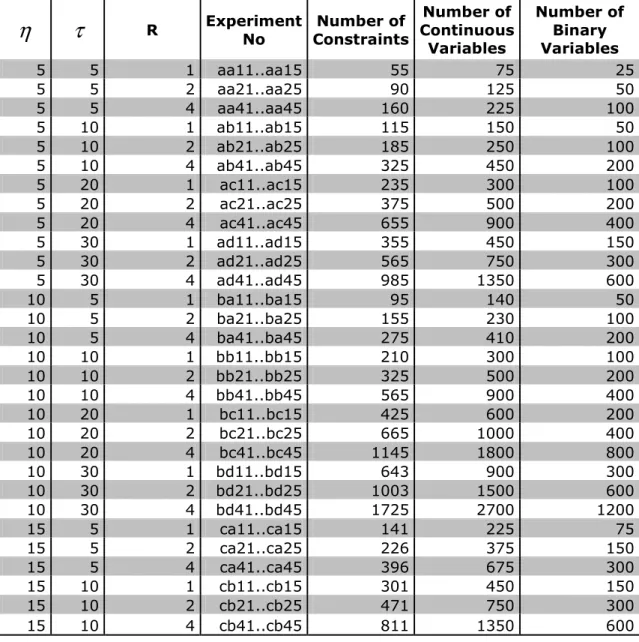
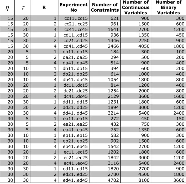
In Table 4-5a and Table 4-5b, we present number of constraints, number of continuous variables and number of binary variables for each experiment set.

η

τ

R Experiment No Number of Constraints Number of Continuous Variables Number of Binary Variables 5 5 1 aa11..aa15 55 75 25 5 5 2 aa21..aa25 90 125 50 5 5 4 aa41..aa45 160 225 100 5 10 1 ab11..ab15 115 150 50 5 10 2 ab21..ab25 185 250 100 5 10 4 ab41..ab45 325 450 200 5 20 1 ac11..ac15 235 300 100 5 20 2 ac21..ac25 375 500 200 5 20 4 ac41..ac45 655 900 400 5 30 1 ad11..ad15 355 450 150 5 30 2 ad21..ad25 565 750 300 5 30 4 ad41..ad45 985 1350 600 10 5 1 ba11..ba15 95 140 50 10 5 2 ba21..ba25 155 230 100 10 5 4 ba41..ba45 275 410 200 10 10 1 bb11..bb15 210 300 100 10 10 2 bb21..bb25 325 500 200 10 10 4 bb41..bb45 565 900 400 10 20 1 bc11..bc15 425 600 200 10 20 2 bc21..bc25 665 1000 400 10 20 4 bc41..bc45 1145 1800 800 10 30 1 bd11..bd15 643 900 300 10 30 2 bd21..bd25 1003 1500 600 10 30 4 bd41..bd45 1725 2700 1200 15 5 1 ca11..ca15 141 225 75 15 5 2 ca21..ca25 226 375 150 15 5 4 ca41..ca45 396 675 300 15 10 1 cb11..cb15 301 450 150 15 10 2 cb21..cb25 471 750 300 15 10 4 cb41..cb45 811 1350 600

(54)

η

τ

R Experiment No Number of Constraints Number of Continuous Variables Number of Binary Variables 15 20 1 cc11..cc15 621 900 300 15 20 2 cc21..cc25 961 1500 600 15 20 4 cc41..cc45 1641 2700 1200 15 30 1 cd11..cd15 936 1350 450 15 30 2 cd21..cd25 1446 2250 900 15 30 4 cd41..cd45 2466 4050 1800 20 5 1 da11..da15 184 300 100 20 5 2 da21..da25 294 500 200 20 5 4 da41..da45 514 900 400 20 10 1 db11..db15 394 600 200 20 10 2 db21..db25 614 1000 400 20 10 4 db41..db45 1054 1800 800 20 20 1 dc11..dc15 814 1200 400 20 20 2 dc21..dc25 1254 2000 800 20 20 4 dc41..dc45 2129 3600 1600 20 30 1 dd11..dd15 1231 1800 600 20 30 2 dd21..dd25 1894 3000 1200 20 30 4 dd41..dd45 3214 5400 2400 30 5 1 ea11..ea15 272 450 150 30 5 2 ea21..ea25 432 750 300 30 5 4 ea41..ea45 752 1350 600 30 10 1 eb11..eb15 582 900 300 30 10 2 eb21..eb25 902 1500 600 30 10 4 eb41..eb45 1542 2700 1200 30 20 1 ec11..ec15 1202 1800 600 30 20 2 ec21..ec25 1842 3000 1200 30 20 4 ec41..ec45 3116 5400 2400 30 30 1 ed11..ed15 1820 2700 900 30 30 2 ed21..ed25 2780 4500 1800 30 30 4 ed41..ed45 4702 8100 3600

(55)

4.3 Comments on Computational Results

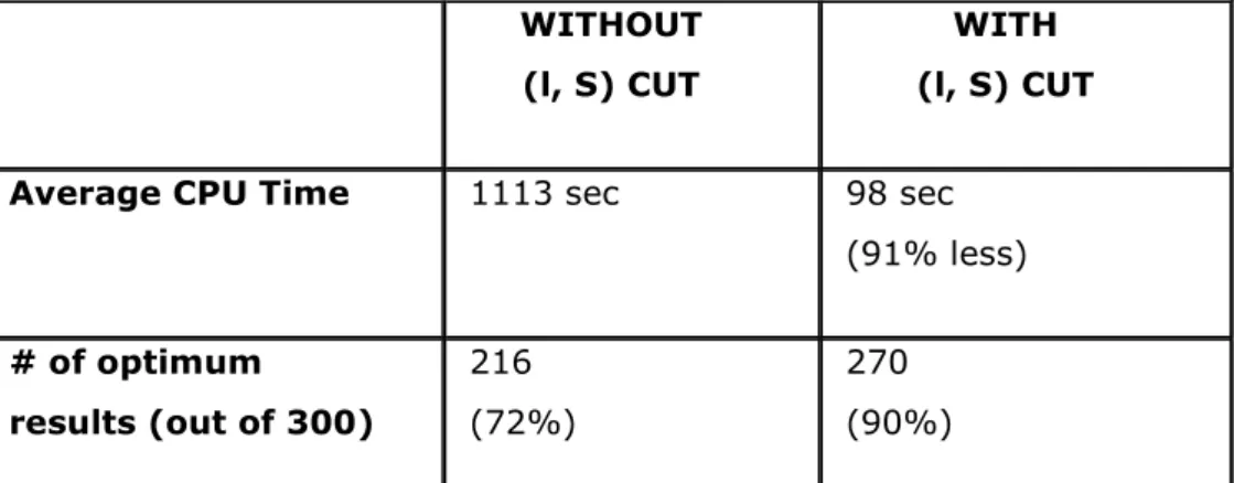
Total time spent to run original problem (without branch-and-cut) is 79.601 sec. (265,3 on the average). However, we spend 35.302 sec to run our algorithm (117,7 on the average). In 236 test instances, original problem (OP) and our algorithm (BC) provide same results. In 191 of them (80%), BC gives faster results. OP reaches 216 optimum results in 3600 sec, whilst BC reaches 270 (90%) optimum results in 300 sec.

Table 4-6 demonstrates the overall results gathered from 300-experiments. When we do append (l, S) cuts, average CPU time decreases by 91%. Additionally, our solution reaches 90% optimality in 300sec with respect to 72% (in case when we do not append (l,S)-cuts) in 3600sec.

WITHOUT

(l, S) CUT

WITH (l, S) CUT

Average CPU Time 1113 sec 98 sec (91% less) # of optimum results (out of 300) 216 (72%) 270 (90%)

Table 4-6 Summary of Computational Experiments

Table 4-7 demonstrates another statistical information on computational experiments. Same solution column represents number

(56)

of experiments in which we get same results when we apply our algorithm and we do not apply our algorithm. In case our algorithm provides better solutions, we add them under “Better Solution” column. Similar operation is performed for “Worse Solution” column. In first row of the table, the results of all instances are demonstrated. In second row, we only demonstrated the experiments which are non-trivial. (mostly when R = 4)

Same Solution Better Solution Worse Solution Over 300-instances 250 (83%) 32 (11%) 18 (6%) Over non-trivial instances (over 50) 20 (40%) 23 (46%) 7 (14%)

(57)

C h a p t e r 5

Conclusion

In this study, we have introduced a lot-sizing problem applicable to the petroleum sector. Our aim is to find a feasible production schedule satisfying customer demand whilst having minimum cost. The capacity restrictions of the plants, chemical and physical properties of the petroleum bring too many constraints to our problem causing difficulty to solve optimally in many cases.

First, we give the description of our problem and present mathematical formulation of it. Then, since this is NP-hard, in order to solve the problem optimally in a reasonable amount of time, we introduce an algorithm, which is based on the branch-and-cut technique. This technique is based on appending (l, S) cuts to the nodes in which we generate convex hull for each item. After the explanation of the algorithm and cuts added, we provide graphical illustration of the proposed algorithm –applied on small data set– to figure out how the

An application of capacitated lot-sizing model in petroleum sector