T.C.
ISTANBUL AYDIN UNIVERSITY
INSTITUTE OF NATURAL AND APPLIED SCIENCES
FEATURE SELECTION FOR LEAF DISEASES DETECTION USING OPTIMIZATION ALGORITHMS
THESIS
Lamyae GOUBRAIM
Department of Electrical and Electronics Engineering Electrical and Electronics Engineering Program
Thesis Advisor: Assist. Prof. Dr. Necip Gökhan KASAPOĞLU
T.C.
ISTANBUL AYDIN UNIVERSITY
INSTITUTE OF SCIENCE AND TECHNOLOGY
FEATURE SELECTION FOR LEAF DISEASES DETECTION USING OPTIMIZATION ALGORITHMS
THESIS
Lamyae GOUBRAIM (Y1613.300021)
Department of Electrical and Electronics Engineering Electrical and Electronics Engineering Program
Thesis Advisor: Assist. Prof. Dr. Necip Gökhan KASAPOĞLU
DECLARATION
I hereby declare that all information in this thesis document has been obtained and presented in accordance with academic rules and ethical conduct. I also declare that, as required by these rules and conduct, I have fully cited and referenced all material and results, which are not original to this thesis.
FOREWORD
After thanks to Allah our creator, I would like to express my gratitude to my advisor, Dr. Necip Gökhan Kasapoğlu. I thank him for framing, guiding, helping and advising me.
I extend my sincere thanks to all the teachers, speakers and all the people who by their words, their writings, their advice and their critics guided my thoughts and agreed to meet me and answer my questions during my research.
I would like to thank my dear parents, who have always been there for me. I thank my sister, and my brothers for their encouragement.
Finally, I would like to thank my friends who have always been there for me. Their unconditional support and encouragement have been of great help.
June, 2019 Eng. Lamyae GOUBRAIM
TABLE OF CONTENT
Page
FOREWORD ... vii
TABLE OF CONTENT ... ix
ABBREVIATIONS ... xi
LIST OF FIGURES ... xiii
LIST OF TABLES ... xv
ABSTRACT ... xvii
ÖZET ... xix
1. INTRODUCTION ... 1
1.1 Machine Learning and Artificial Intelligence ... 2
1.2 Problem Definition ... 2 1.3 Previous works ... 3 1.4 Motivation ... 7 2. PRE-PROCESSING STEPS: ... 9 2.1 Feature extraction ... 9 2.2 Pre-processing ... 11
2.3 LAB color space ... 14
2.4 K-means clustering method ... 15
3. FEATURE SELECTION ... 19
3.1 Introduction of Imperialist competitive algorithm (ICA) ... 22
3.2 Particle swarm optimization (PSO) ... 25
3.3 Mathematical Model of PSO ... 28
3.4 The comparison between ICA and PSO ... 30
3.5 Using Imperialist competitive algorithm ... 30
3.6 Using Particle swarm optimization PSO ... 31
4. DECISION MAKING ... 35
4.1 Artificial neural network (ANN) ... 36
5. DESIGNED EXPERIMENTS AND RESULTS ... 41
5.1 Designed experiments ... 41
5.2 Accuracy of PSO and ICA ... 57
5.3 Conclusion and future work ... 61
6. REFERENCES ... 63
ABBREVIATIONS
ANN :Artificial Neural Network
ICA :Imperialist Competitive Algorithm PSO :Particle Swarm Optimization PCA :Principal Component Analysis GA :Genetic Algorithm
KNN :K-nearest neighbor SVM :Support Vector Machine SGDM :Gray-level Dependence Matrix RGB :Red Green Blue
HSV :Hue Saturation and Value channel PRR :Phytophthora Root Rot
CLR :Coffee Leaf Rust CWD :Coffee Wilt Disease CBD :Coffee Berry Disease
BPNN :Back Propagation Neural Network CNN :Deep Convolution Networks MSE :Mean Square Error
LIST OF FIGURES
Page
Figure 2.1: Various diseases in plant leaf. ... 12
Figure 2.2: Original image in RGB ... 12
Figure 2.3:Image in LAB color domain ... 12
Figure 2.4: K-means clustering and layer selection process. (a) Original image, (b) Kmeans results for K=3 and 1st and 2nd layers of LAB (Layers L and A), (c) K-means results for K=3 and 2nd and 3rd layers of LAB (Layers A and B), (d) K-means results for K=4 and 2 ... 13
Figure 2.5: Segmented image in color. ... 14
Figure 2.6: CIELAB color space... 15
Figure 2.7: Flow chart of K mean algorithm. ... 16
Figure 2,8: Flow chart of the preprocessing phase. ... 17
Figure 3.1: ICA workflow to select discriminative features ... 21
Figure 3.2: Movement of colony... 23
Figure 3.3: The competition of empires: the most powerful empire is more likely to have the weakest colony of the weakest empire ... 24
Figure 3.4 General flow chart of ICA. ... 25
Figure 3.5: General Flow chart of Particle Swarm Optimization (PSO). ... 27
Figure 3.6: Mathematical model of PSO ... 28
Figure 3.7: Simple Model of Moving Particle Some considerations are necessary to complete the standards of PSO: ... 29
Figure 3.8: Example of convergence curve of best cost giving by ICA in each iteration from 0 to 1000 ... 31
Figure 3.9: The way PSO works to select optimal features ... 32
Figure 3.10: Example of convergence curve of best cost giving by PSO in each iteration from 0 to 1000 ... 33
Figure 4.1: Artificial neural network system ... 36
Figure 4.2: The proposed method of selecting optimal features ... 38
Figure 4.3: The percentage of samples in each class (The ANN‟s output) ... 39
Figure 5.1: Validation performance of Experiment 1 by ICA in each trail ... 43
Figure 5.2: Training performance of Experiment 1 by ICA in each trail ... 43
Figure 5.3: Testing performance of Experiment 1 by ICA in each trail ... 43
Figure 5.4:: gradient of Experiment 1 by ICA in each trail ... 44
Figure 5.5: The best cost of Experiment 1 by ICA in each trail ... 44
Figure 5.6: Validation performance of Experiment 2 by ICA in each trail ... 46
Figure 5.7: Training performance of Experiment 2 by ICA in each trail ... 46
Figure 5.8: Testing performance of Experiment 2 by ICA in each trail. ... 46
Figure 5.9: The gradient of Experiment 2 by ICA in each trail. ... 47
Figure 5.10: Gradient of Experiment 2 by ICA in each trail ... 47
Figure 5.11: Validation performance of Experiment 1 by PSO in each trail ... 49
Figure 5.12: Training performance of Experiment 1 by PSO in each trail ... 49
Figure 5.14: Gradient of Experiment 1 by PSO in each trail ... 50
Figure 5.15: Best cost of Experiment 1 by PSO in each trail ... 50
Figure 5.16: Training performance of Experiment 2 by PSO in each trail ... 51
Figure 5.17: validation performance of Experiment by PSO in each trail ... 52
Figure 5.18: Testing performance of Experiment 2 by PSO in each trail ... 52
Figure 5.19: Best Cost of Experiment 2 by PSO in each trail ... 52
Figure 5.20: Gradient of Experiment 2 by PSO in each trail ... 53
Figure 5.21: ICA mean convergence for the selected features ... 56
Figure 5.22: ANN training Performance for the selected features ... 56
LIST OF TABLES
Page
Table 3.1: parameter of ICA used in this work ... 22
Table 4.1: Parameters of ANN used in this work ... 36
Table 5.1:10 trails done by ANN with ICA algorithm 20% testing 60% training and 20% validation. ... 42
Table 5.2: Nine trails done by ANN with ICA algorithm 15% testing 70% training and 15% validation ... 45
Table 5.3: 10 trails done by ANN with PSO algorithm 20% testing 60% training .. 48
Table 5.4::9 trails done by ANN with PSO algorithm 15% testing 70% training and15% validation. ... 51
Table 5.5: The average of validation, testing, training and best cost in each trail of both experiments with ICA algorithm ... 55
Table 5.6: Confusion Matrix using 9 features ... 59
Table 5.7: Confusion Matrix using 5 features (ICA result) ... 60
Table 5.8: Confusion matrix using features (PSO result) ... 60
FEATURE SELECTION FOR LEAF DISEASES DETECTION USING OPTIMIZATION ALGORITHMS
ABSTRACT
Modern techniques of computer science and machine learning become more and more important and useful in recent years. The cutting-edge techniques of artificial intelligence assisted humanity in different aspects of life, such as health-care, military and agricultural fields. However, a current solution of identifying leaves diseases totally based on visual inspection of farmers and agricultural engineers. Because this is a very time consuming manual method, its cost is also high as it requires a lot of personnel and risks a lot of plants. This work proposes a novel solution to identify the location and type of diseases on plant leaves, using imperialist competitive algorithm (ICA) for feature selection, and an efficient artificial neural network (ANN) algorithm for recognition. Moreover the comparison between two meta-heuristic optimization algorithms namely imperialist competitive algorithm (ICA) and particle swarm optimization (PSO) is given to demonstrate the effectiveness of the ICA.
Keywords: Artificial neural network (ANN), feature selection, imperialist
competitive algorithm (ICA), meta-heuristic, particle swarm optimization (PSO), plant leaf disease recognition.
YAYILMACI REKABETÇİ ALGORİTMASINI KULLANARAK BİTKİ YAPRAK HASTALIKLARININ BELİRLENMESİ
ÖZET
Modern bilgisayar bilimi ve makine öğrenmesi teknikleri son yıllarda giderek daha önemli ve kullanışlı hale gelmiştir. Yapay zekanın en ileri teknikleri, sağlık, askeri ve tarım alanları gibi yaşamın farklı yönlerinde insanlığa yardımcı olmaktadır. Bununla birlikte, bitki yaprak hastalıklarının tespitinde mevcut çözümler tamamen çiftçilerin ve ziraat mühendislerinin görsel incelemesine dayanmaktadır. Bu çok yavaş bir yöntem olduğundan, maliyeti çok yüksektir, çünkü çok sayıda personel gerektirir ve çok sayıda bitkinin hastalanması riskini taşır. Bu tezde, bitki yaprakları üzerindeki hastalıkların yerini ve türünü tanımlamak için, öznitelik seçimi için yayılımcı rekabet algoritması (YRA) ve tanıma için verimli bir yapay sinir ağı (YSA) algoritması kullanarak yeni bir çözüm önerilmektedir. Ayrıca, yayılımcı rekabet algoritması (YRA) ve parçacık sürüsü optimizasyonu (PSO) gibi iki sezgisel optimizasyon algoritması arasındaki karşılaştırma, YRA' nın etkinliğini göstermek için verilmiştir. Anahtar Kelimeler: Yapay sinir ağları (YSA), öznitelik seçimi, yayılmacı rekabetçi
algoritması (YRA), sezgisel yöntemler, parçacık sürüsü optimizasyonu (PSO), bitki yaprak hastalıklarının tanınması.
1. INTRODUCTION
State-of-the-art automated techniques can be used to achieve more advanced and accurate solutions that can reduce costs to detect leaves diseases in a shorter time. However, in some previous studies some methods proposed to solve the same problem, but in these studies proper features have to be used to achieve more accurate results have been ignored. In this thesis imperialist competitive algorithm (ICA) is used with cascade feed forward neural network to extract the most suitable features to be used in detecting diseases in leaves. Diseases considered in this study are alternaria alternate, anthracnose, bacterial blight, septoria brown spot and cercospora.
Alternaria alternata is a fungus or mushroom which has been recorded causing leaf spot and other diseases on over 380 host species of plant. It is an opportunistic pathogen on numerous hosts causing leaf spots, roots, and blights on many plant elements [1]. Moreover, anthracnose is a fungal disease that develops when the humidity is too high, especially in spring and autumn, but also in summer [2].
Bacterial blight is the most common soybean disease in cold, wet weather. This disease usually occurs at low levels that do not lead to a loss of yield. The bacterial blight may be mistaken for the septoria brown spot. An error can be made in the distinction between bacterial blight and septoria brown spot. These two diseases can be distinguished by the presence of a halo around bacterial lesions. Same plant can be exposed to both diseases at the same time, However bacterial blight are more common in young leaves, as long as brown spots usually occur on older leaves and less leaves. [3].
On the other hand, cercospora fruit spot is a common disease of citrus fruits but it also affects many other crops. The disease is fungal and survives on any affected fruit in soil from the previous season [4].
These diseases can infect several types of plants, such as bean, beetroot, capsicum, okra, silver beet, watercress, carrot, avocado and coffee in different
regions around the world, especially in South East Asia and Africa. These diseases are usually detected manually by farmers or agricultural engineers who survey the fields. However, due to the advanced technologies of computer science and machine learning, the cutting-edge methods of image processing are becoming widely used to replace traditional methods efficiently.
1.1 Machine Learning and Artificial Intelligence
Machine Learning is the science of getting a computer to act based on a model built during the training. It has two sub-fields and artificial intelligence is the most important one. Machine Learning is the simulation of human intelligence by means of machines. Those approaches consist of learning (the acquisition of information and rules for the use of the information), reasoning (the use of the rules to reach approximate or definite conclusions) and self-correction. Moreover, artificial intelligence has mains applications such as:
• Prediction is the ability to learn and predict future events, without being explicitly programmed.
• Sample recognition is a branch of machine learning that emphasizes the recognition of data patterns or data regularities in a given scenario.
• Clustering: is a machine learning technique that involves the grouping of data factors. Given a set of statistics factors, we can use a clustering algorithm to categorize each data point into a specific group.
In artificial intelligence several algorithms are used such as fuzzy logics a form of many-valued logic in which the real values of variables may be any real number between 0 and 1. It is hired to deal with the concept of partial reality, where the real value may range between completely true and completely false. Additionally, artificial neural network popularly known as neural community is a computational model based on the structure and functions of biological neural.
1.2 Problem Definition
There are several types of diseases affect plants and their leaves. However, traditional methods that are based on individual’s observations are accurate, but
may take long time. In addition to this as in large fields where there are huge range of plants or trees, this traditional method may take very long time which can cause the plants to reach a worst situation before the disease being detected. Currently, computer science and machine learning techniques are used in this field and these techniques supply promising results. Nevertheless, the existing solutions lack the accuracy and speed of the detection procedure, which is usually due to the wide variety of features available at the back of the plant leaf image. Additionally, the previous works may not be able to identify the most suitable feature to be used, which reflects on the overall system performance. Therefore, it is important to discover a solution that provides the processing algorithm with suitable features, to have accurate disease detection within relatively shorter time.
1.3 Previous works
In this section, we review some previous works related to the plant leaf disease recognition in order to outline the performance of the algorithms. Singh and Misra [5] have tackled the problem of diseased plants and the delay usually experienced before imparting proper medication using traditional techniques. They have proposed an algorithm to provide proper segmentation for the leaf image and automatic detection for plant leaf disease. They have focused on one disease which is the little leaf in pine trees. They have conducted their research on samples collected from the United States. In order to implement their proposed solution, they have used genetic algorithm (GA) for image segmentation and made comparison between two methods which are K-means and support vector machine (SVM). They have extracted features using gray level co-occurrence matrix. In this paper smoothing filter is implemented as in pre-processing stage and to increase the contrast image enhancement. A digital camera is used for the image capturing. They have concluded that using genetic algorithm reduces the performance of this work. Max 15 images per sample were used in this study may be not sufficient to build a model and making performance evaluation.
Sabanb and Bayramin proposed a hybrid neural network for segmentation of leaf images [6]. Automatic segmentation method is proposed using four unique
color components. In order to implement their proposed method, various illumination conditions is used for image segmentation and the image is converted into RGB, HSV, XYZ and YIQ channels. After the transformation of the color components, B, S, Z and I components are used to train hybrid neural network and color features are extracted from each color region. Trained artificial neural network using gray wolf algorithm on the selected features was obtained. They have reported outperformed results according to sensitivity, specificity and accuracy.
Khirade and Patil handled the problem of monitoring plant diseases [7]. They proposed a method for detecting plant diseases using their leaves images. They focused on some specific disease such as powdery mildew yellow rust and aphids diseases. They have collected their images using a digital camera. In their proposed solution they have used the boundary and spot detection to identify infected parts of a leaf. They employed co-occurrence texture futures in K-means clustering algorithm for image segmentation. In this work the classification is applied using artificial neural network (ANN) with back propagation learning. Clipping smoothing and enhancement are applied as preprocessing step to remove noise in images.
Image processing is used for detection of diseases in cotton leaves [8]. In this work principal component analysis (PCA) and K-nearest neighbor (KNN) classifier are used in order to identify diseases. In this study the aim is to recognize diseases such as blight, leaf nacrosis, gray mildew, alternaria and magnesium deficiency. The most substantial capabilities from 110 samples were extracted and compressed to keep only the significant information. The accuracy of the proposed PCA-KNN based classifier is reported as 95% in this work.
In [9], the authors have tackled the problem of distinguishing plant leaves from their environment. Their technique is based on leaf image classification using deep convolution networks (CNN). The model built in this study is able to recognize thirteen different types of plant diseases such as powdery mildew, taphrina de formans, pear, erwinia amylovora. All the images used in the work are collected from the internet. The precision of the proposed method were reported between 91% and 98%.
The problem of diseases plants is the subject of the study in [10]. In this study neural network with back propagation (NN-BP) learning, k-way clustering and spatial graylevel dependence matrix (SGDM) have been used to analyses healthy and diseased plant leaves. In order to implement proposed scheme k-method clustering algorithm are applied for image segmentation and the masked cells inside the boundaries of the infected clusters are removed. The infected cluster is converted from RGB to HSI space. In this study neural networks (NN) have been used for recognition. Total 118 diseased leaf samples were used in the experiments. Proposed method is reported good potential with an ability to detect plant leaf diseases with some limitations.
Yahya et al.[11] studied the problem of detecting plant diseases. They have proposed a spectroscopy technique that has grown to be one of the most available noninvasive methods utilized in detecting plant diseases. They collected the images using digital camera to enhance the accuracy of their work. They have centered on a lot of diseases such as yellow rust, bacterial canker, downy mildew, apple scab, they have tested the 3 major categories for noninvasive monitoring of plant diseases which might be the visible and infrared spectroscopy (VIS/IR) technique. These categories are impedance spectroscopy (IS)and fluorescence spectroscopy (FS) techniques. They have concluded that spectroscopy strategies have the potential to be applied on plants, as a noninvasive disorder detecting tool.
In [12] the authors have tackled the problem of Phytophthora root rot (PRR) which infects the roots of avocado trees. In their paper they proposed two image analysis methods that can serve as surrogates to the visible assessment of canopy decline in large avocado orchards. These methods are combination of Canny edge detection and
Otsu‟s method. Coinciding with the on-floor measure of cover porosity, they have used a total of 80 bushes to gather samples from three avocado blocks. In this study a smart phone camera was used to collect RGB color images.
Identification of coffee plant diseases that attack coffee plants using hybrid approaches of image processing and decision tree has been introduced in [13]. The authors have focused on the three foremost of diseases such as coffee leaf rust (CLR), coffee berry disease (CBD) and coffee wilt disease (CWD). They
have proposed back propagation artificial neural network (BPNN) as technique to recognize diseases. In their work they have used K-means clustering for image segmentation within the first stage of their paper coffee plant diseases are given as input to the system. The second step is that pre-processing of images, such as median filtering is used in this step for reducing noise. They have reported 94.5% of accuracy in their work.
Sivakamasundari and Seenivasagam have worked to provide a fast and cheap solution for detecting apple leaf diseases at the earlier stage. The authors have proposed a system aims to identify a number of the diseases in apple leaf based on color and texture feature. The diseases chosen are alternaria, apple scab, and cedar rust. In order to put in force their work; they have used K-means clustering for image segmentation; gray-level co-occurrence matrix (GLCM) or grey level spatial dependence matrix is used for texture evaluation. They have concluded that the accuracy in their paintings according to texture and color future is high therefore in the future the same system can be used to test other kinds of plants.
JUse of plant models in deep learning is proposed in [15]. The authors have proposed a new technique for augmenting plant phenotyping datasets using rendered images of synthetic plants by using computer-generated model of the arabidopsis rosette to enhancing leaf counting performance with convolutional neural networks (CNNs) and they have mainly focused on rosette plants.
Sunny and Gandhi have tackled the problem of citrus plants such as lemon which are mainly affected by citrus canker disease which affects the fruit production of the plants [16]. They have proposed an image processing technique to detect plant leaf diseases from digital images. The proposed method involves stages using contrast limited adaptive histogram equalization (CLAHE) enhancement and SVM classifiers to improve the clarity of leaf images. They have mainly focused on citrus canker disease. Images are captured by high resolution digital camera and they have used 100 samples in their work. In this approach, leave image features include texture, color, shape are taken into consideration for disease detection. They have concluded that the pre-processing step with CLAHE enhancement achieves efficient result integrated
with SVM classifiers. The SVM classifiers achieve the good prediction rate for differentiating the canker disease.
1.4 Motivation
The aim of this thesis is to select the most distinctive features that increase the recognition accuracy of the leaf diseases. An enhanced technique is proposed based on optimization algorithm to accurately discover the most suitable features to be extracted in the fields of diseases image classification. In this thesis to identify the most efficient algorithm to be used in selecting the disease features in leaf images is implemented and an approach that provides an enhanced detection accuracy and recognition quality is proposed. In order to reach thesis aims this work tries to find solutions for research questions below. Q1- Is it possible to use an optimization algorithm to identify the most optimal features to be used by ANN for the classification process?
Q2- Does the use of an optimization algorithm, as a feature selector for the ANN, improves the accuracy of leaf diseases detection?
2. PRE-PROCESSING STEPS:
2.1 Feature extraction
Features are defined as a function of one or more measurements, each of which specifies some quantifiable property of an object. There are various features which are classified into:
• General features: Independent features such as color, texture , and shape.
According to the abstraction level, they can also be divided into:
• Pixel-level features: Features calculated at each pixel, such as color. • Global features: Calculated over the entire image or on a regular
sub-area of an image.
• Domain-specific features: Applying dependent features such as human faces, fingerprints, and conceptual ones.
• Local features: They are calculated on the results of the subdivision of the image segmentation or edge detection.
All features can be roughly classified into low-level and high-level features. Lowlevel features can be extracted directly from the original images, while extraction of high-level features depends on low-level features.
In this work gray level co-occurrence matrix (GLCM) feature extraction method is used to extract nine features after converting the segmented image to gray level. A Matlab code of the method is given below:
GrayImg=rgb2gray(ImgSeg);
GrayCooccurance=graycomatrix(GrayImg);
ImageFeatures=graycoprops(GrayCooccurance,'Contrast Correlation Energy Homogeneity');
Asymmetry=[asymmetry,skewness(double(ImgSeg(:)))]; Avg=[Avg,mean2(ImgSeg)];
ISTD=[ISTD,std2(ImgSeg)]; Shaprness=[Shaprness,kurtosis(double(ImgSeg(:)))]; RMS=[RMS,mean2(rms(ImgSeg))]; ImgVar=[ImgVar,mean2(var(double(ImgSeg(:))))]; ImageE=[ImageE, entropy(ImgSeg)]; ImgSummation=[ImgSummation,sum(double(ImgSeg(:)))]; ImageSmooth=[ImageSmooth,1-(1/(1+ImgSummation(n)))];
The extracted features for this work are as follows: • Texture features:
RMS: The root mean square is a measure of the magnitude of a set of numbers. It gives a sense for the typical size of the numbers [16].
Image Smoothing: Smoothing is often used to reduce noise within an image or to produce a less pixelated image. The most of the smoothing methods are based on low pass filters [17].
Skewness: Skewness is a measure of the asymmetry of the gray levels around the sample mean. If skewness is negative, the data are spread out more to the left of the mean than to the right. If skewness is positive, the data are spread out more to the right [18].
Kurtosis: Kurtosis is a measure of how outlier-prone a distribution is. It describes the shape of the tail of the histogram [19].
Entropy: Entropy of the image is the measure of randomness of the image gray levels [20].
• Color features:
Standard deviation ISTD: Standard deviation of the intensity values (ISTD) is calculated for this color feature as follows: [21]:
(2.1) where is intensity value for pixel i and is the mean value of an image or subimage.
Average: The mean gives the average gray level of each region and it is useful only as a rough idea of intensity not really texture [22].
(2.2)
where A is average or arithmetic mean., n is the number of samples and is pixel intensity value for pixel i..
Image Variance: The variance gives the amount of gray level fluctuations from the mean gray level value [23].
(2.3)
Image Sum: Image sum is to take the sum of the intensities of the pixels in an image.
2.2 Pre-processing
Generally to create a neural network in Matlab, the network is composed of n inputs, n outputs and a number of hidden layers.
The first step is to set the input and output nodes and the network is designed as follow, setting the number of hidden neurons and outputs once the activations functions are also cited the training function is defined with some training parameters such as number of epochs, validation checks…etc, Furthermore once the network is trained in the training process then all the performance measures
such as the training performance, are given. Moreover the execution time and the training process to reach the goal performance are also given by neural network.
In our case, our aim is to identify some of the diseases in plant leaves based on selected features by imperialist competitive algorithm (ICA) and Particle Swarm Optimization (PSO). The code is written in Matlab.
Alternaria Alterana Anthracnose Bacterial Bright Cercospora Leaf
Figure 2.1: Various diseases in plant leaf.
In image acquisition step, the images are read one by one by using IMREAD function, then in the image pre-processing step some adjustments are applied on the images to enhance their quality in order to make it more clarify for processing ,
IMRESIZE function is also used to convert images to 256*256, IMADJUST function is used to have all the images in the full-screen of the figure. Moreover we convert the images from RGB domain (see Fig. 2) to LAB color domain using SRGB2LAB function as shown in Fig 3.
Figure 2.2: Original image in RGB Figure 2.3:Image in LAB color domain
After the images has been transformed to LAB color domain (CForm) the segmentation is implemented using K-means clustering algorithm. However,
Kmeans works on data not images. It clusters the data based on the distances of similarities between the neighbors. Thus, the goal is to reshape the image into vector data not image and then it is clustered with K-means algorithm. Knowing that two column vectors (layers) the layer A and the B from LAB color space, are included from the four clusters, the aim is to put each layer in a column in this vector of data in order to isolate the region of interest. The details of the method is given as follows:
• The layer A and B are extracted then the image are reshaped into vector with two columns.
• K-means clustering is done by choosing the number of clusters, the selected layers will be divided in four because more accurate result appears when K=4 clusters are chosen on layers A and B otherwise the region of interest are mixed with the background.
• Then the K-means clusters for the selected layers which are 2 and 3 are stored the segmented pixels in Matlab variable CIndex. Obtained clusters are shown in Figure 4.
(a) (b) (c)
(d) (e)
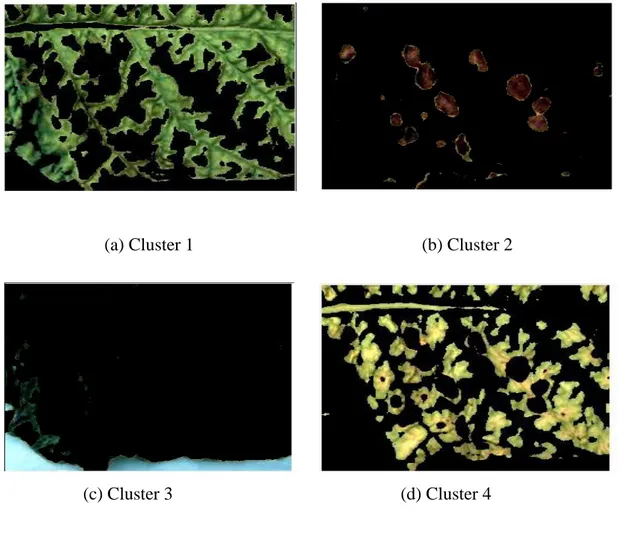
Figure 2.4: K-means clustering and layer selection process. (a) Original image, (b) Kmeans results for K=3 and 1st and 2nd layers of LAB (Layers L and A), (c)
means results for K=3 and 2nd and 3rd layers of LAB (Layers A and B), (d) K-means results for K=4 and 2
Hence, two layers are conducted from 3 layers of LAB color space, important results appeared when layers A and B was divided into four clusters, as shown in Figure 4(d).
(c) Cluster 3 (d) Cluster 4
Figure 2.5: Segmented image in color.
Figure 5 shows results of segmented image in color obtained by K-means clustering, the four classes are sited and each ones represent a separate range of colors, hence cluster 2 shows only the region of interest which is the disease part.
2.3 LAB color space
This space is also known as CIELAB (see Figure 6) and CIELAB contains three layers: The L axis reproduces the brightness, the A axis is responsible for the orangered hues and greens while the B axis describes the colors from blue to yellow. The color model is hardware independent. Colors are defined regardless
1
of how they are produced and their reproduction technique. The LAB color space is a uniform color space, thus the greater the distance between the colors in the color space, the more the color difference becomes clear for the eye. All the color information is in the A and B layers.
Figure 2.6: CIELAB color space
2.4 K-means clustering method
K-means is one of the most common clustering algorithms. It makes possible to analyze a set of data characterized by a set of descriptors, in order to group the "similar" data into groups or clusters.
The similarity between two data can be inferred from the "distance" separating their descriptors, thus two very similar data are two data whose descriptors are very close. This definition makes it possible to formulate the data partitioning problem as the search for K "prototype data", around which the other data can be grouped.
Figure 2.7: Flow chart of K mean algorithm.
The algorithm starts by choosing K initial cluster centers of K groups then place the objects in the group of nearest center then recalculate the center of gravity from each group. In addition of those steps the algorithm iterates until the cluster centers stops to change anymore groups (see Figure 7).
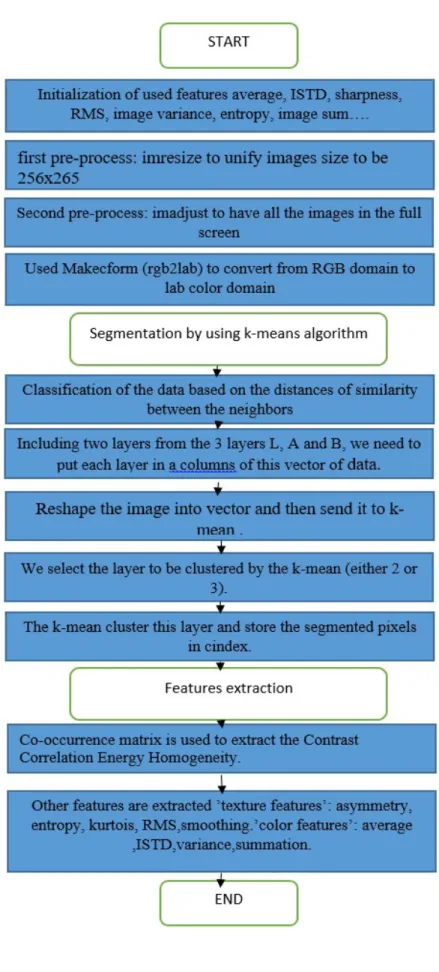
In the proposed method there are 3 steps and the following flowchart explains the first step of our work which is pre-processing step, starting by initializing all features intended to be used in this study after that some adjustments are applied to the size of images and their quality to have all the images in a full screen and also to unify the images size to 256*256, then the images are converted from RGB domain to LAB color domain. Moreover the segmentation step is implemented using K-means clustering which classify the data on the distances of similarities between neighbors, in the end of segmentation step the k-mean cluster the selected layer and stored the segmented pixels in CIndex (variable chosen to store the segmented pixels on Matlab code). By the end of the preprocessing step the nine features that will be processed by ICA are extracted.
3. FEATURE SELECTION
In order to select the most discriminative features, an optimization algorithm is used. In this thesis imperialist competitive algorithm (ICA) is chosen for selection of discriminative features. The role of ICA is to choose the optimal features within 9 used features and the algorithm consists of two competition mechanisms:
• The intra-empire competition is competition between members of an empire,
• The inter-empire competition is the competition within empires, according to the overall objective value of the empire. Within the empire, the strongest country will be the imperialist (the leader) of the whole empire; It is the intra-empire competition.
• The optimization aim is to find an optimal solution in terms of problem variables. We form an array of variable values to be optimized.
• In Genetic Algorithm (GA) terminology, this array is called “chromosome”, but here the term “country” is used for this array. In our proposed method 9 features are chosen as variables such are:
• color features: average, standard deviation, variance, summation • texture features: entropy, asymmetry (skewness), kurtosis, RMS,
smoothing
In this thesis the Imperialist competitive algorithm (ICA) and particle swarm optimization (PSO) are used to specify the best features within 9 features to reach the best recognition accuracy.
Employing ICA in this thesis is demonstrated in Figure 9 ,the mean component of the ICA is the agents whose functionalities is to look for new solutions to optimize the problem under study ,in our work the problem is to find the
optimal solution to be used in the Artificial neural network in order for the agents to define the optimal features we have to convert the solutions of these agents to be binary which contains zero and one only ,while 1 means the selected features and 0 means the discarded features each one of the agent in the colony of an empire suggest a solution ,this solution then sent to the cost function which contains our ANN model ,then the MSE
(z= perform(net,Target,y))obtained by the ANN model for the best selected solution will be sent back to the same agent and which will sent it back to the colony that it belongs to ,then the colonies will compare this cost value with others in order to update the imperialist value ,over inside the cost function ,the ANN takes the samples of the selected features and then it is trained on it and test the identified weights values with the testing data set in order to calculate the value of the MSE which then will be identified as a set value of the selected solution for these corresponding agents. Continuing on this way and completing the required iterations it will insure the proposed system to achieve the best position of the optimal solution which presents the optimal combination of features to be used by ANN for the same problem under study.
Figure 3.1: ICA workflow to select discriminative features
Using these parameters illustrated in Table our proposed designed can identified the optimal combination of features to be used in detecting diseases under study.
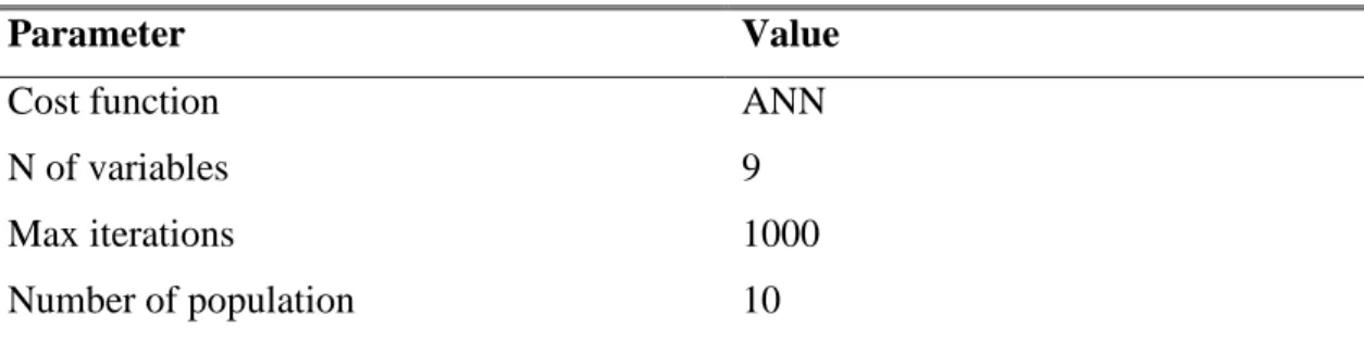
Table 3.1:parameter of ICA used in this work
Parameter Value
Cost function ANN
N of variables 9
Max iterations 1000
Number of population 10
3.1 Introduction of Imperialist competitive algorithm (ICA)
The ICA algorithm was inspired from the idea of imperialism, Hence in this process the powerful countries takes control of the weakest one. Moreover this meta-heuristic algorithm was proposed by Atashpaz-Gargari and Lucas [24], Thus ICA has been used in various applications.
Imperialist competitive algorithm (ICA) is a socio-politically strategy proposed to solve optimization problems, Moreover it is a new meta-heuristic algorithm used to solve some engineering issues which is similar to many other developed algorithm, it starts with a random initial population or empires, each agent in this empires is called country. Countries are categorized into two types as of imperialist and colony. ICA is based on a competition between those, in this competition the powerful empires take the position of their colonies and the weakest ones fall in.
• Imperialist competitive algorithm (ICA)
Initialize and evaluate the empires while Stop condition is not satisfied do Move the colonies toward their relevant imperialist
Revolution. Make some changes in the characteristics of some of the countries if there is a colony in an empire which has lower cost than that of imperialist then
Exchange the positions of that colony and the imperialist end if Compute the total cost of all empires
if the distance between two empires is less than Uniting Threshold then Unite the two empires end if
Imperialistic competition
if there is an empire with no colonies then Eliminate this empire end if end while
Figure 3.2: Movement of colony
Initialization: In the algorithm each individual of the population represents a country, the first step is to initialize and evaluate them. The best countries are selected and become the imperialists and those who are not become imperialist are colonies. Colonies are then spread over the empires according to their power.
Movement: After having divided the colonies among the different imperialists, each colony moves towards its imperialist. Figure 10 illustrates this movement, d is the distance between the colony and the imperialist. θ and x are random numbers. The number θ, drawn randomly, allows slightly deflect the colony. After each movement of a colony, it may be that the cost of a colony is less than the cost of its imperialist, in which case the colony becomes the imperialist. Total cost of an empire: The total cost of an empire depends on the cost of the imperialist and it is colonies. The eqn. (1) gives the expression which makes it possible to calculate the total cost of an empire n.
where ξ is less than 1.
Imperialist competition: Imperialist competition allows a stronger empire to seize of a colony of the weakest empire. This competition makes it possible to increase the power of strong empires and eliminate weak empires. Figure 11 illustrates this competition; the weakest empire 1 is on the verge of losing a colony for the benefit of one of the empires. Each empire has a probability of possession calculated from its power.
Figure 3.3: The competition of empires: the most powerful empire is more likely to
have the weakest colony of the weakest empire
The imperialist competitive algorithm is an evolutionary algorithm, which works on the same way like other population-based algorithms, it starts by initializing the population where the best countries are selected as the imperialist another makes part of the colonies imperialist. All the colonies of the population are distributed on the imperialist countries according to their power.
After dividing all the colonies among the imperialists, the colonies begin to move towards their imperialist countries. The total power of all the empires depends on the power of the imperialist countries and the power of their colonies (the countries with the least cost function value become powerful imperialists and start controlling other countries called colonies, hence the initial imperialist is formed. This fact is defined with the full power of an empire by the power of the imperialist state in addition to the percentage of the
average power of its colonies. The imperialist competition will finish by an increment in the power of the powerful empires and decrement in the weaker empire‟s power. However the empires that cannot remain in this competition and cannot increase its power will be ignored or removed. Nevertheless the weakest empire will collapse one by one while all countries will definitely become a state in which there is only one empire and all the remaining countries are colonies of that empire. General flow chart of ICA is depicted in Figure 12 [24].
Figure 3.4 General flow chart of ICA.
3.2 Particle swarm optimization (PSO)
Particle swarm optimization or PSO is an intelligent optimization algorithm, it belongs to a class of optimization algorithms called meta-heuristic algorithms, and inspired by social behavior of flocking birds and schooling fish. PSO is a simple powerful optimization algorithm applied successfully to an enormous applications in various field in science and engineering such as Machine learning, image processing, data mining and many other fields .Initially PSO is introduced by James Kennedy and Russel Eberhat in 1995 originally, they were working to developed model to describe a social behavior like flock of birds and school of fish. However, they released that their model is capable of doing optimization test so they proposed a new optimizer based on their model just called Particle Swarm Optimization .in those last 20 years PSO became one of the most useful and most popular algorithms to solve various optimization
problems in various field. Despite its simplicity PSO is also a powerful algorithm.
• Algorithm of Particle Swarm Optimization PSO The basic algorithm is very simple:
We denote g the best known position of the swarm and f (x) the function that calculates the criterion of x.
For each particle:
We initialize our position
We initialize its best known position p as its initial position
If f (p) <f (g), we update the best position of the swarm The speed of the particle is initialized.
As long as we have not reached the maximum iteration or a certain value of the criterion: For each particle i:
We draw random c2 and c3
We update the speed of the particle according to the formula seen previously We update the position xi
If f (xi) <f (pi),
We update the best position of the particle
If f (pi) <f (g), we update the best position of the swarm.
The principle of the algorithm can be more easily visualized from the Figure 13.
PSO uses a number of particles called the swarm of candidate solution called particles. These particles are allowed to move around and traverse the search-space.
These particles move to a new position depending to those rules: • The particle‟s own previous velocity (Inertia)
• Distance from the individual particles‟ best known position. • Distance from the swarms best known position (Social Force)
Based on those simple rules the particles will corporate to find the best location in the search space and best solution for the optimization problem.
Figure 3.5: General Flow chart of Particle Swarm Optimization (PSO).
3.3 Mathematical Model of PSO
Figure 3.6: Mathematical model of PSO
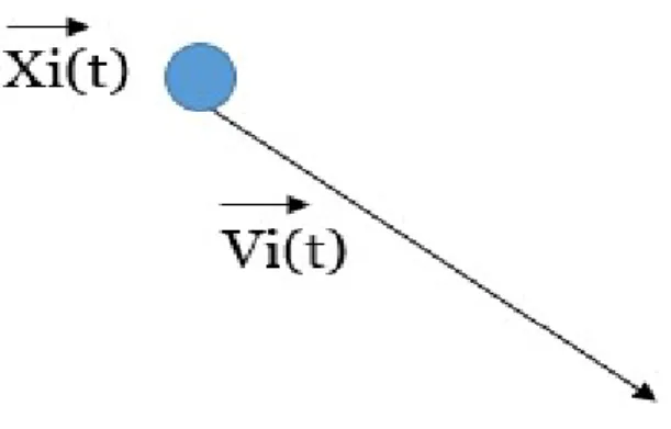
We denote the position of Particle i by and having also velocity for every particle denoted by in a same space as position, the dimension of X and V are same ,the velocity describes the movement of particle (i) in the sense of direction and the sense of distance .thus we have a particle in time step t which is located in the position and it moves towards a vector such as shown in (Figure 14). These particles are interacting and learning from each other or obeying some simple rules to find the best solution for an optimization problem .In addition to position and velocity every particle has a memory of its swarm best position or best experience this is denoted by personal best shown in (Figure 14) We have also a common best experience among a member of swarm denoted by G(t) it hasn‟t index of i because it belongs to the whole swarm ,thus we have personal best for every particle and a global best which is the best experience of all particles in the swarm .The mathematical model of
PSO is very simple by defining these concepts in every iteration of PSO P and V are updated according to this simple mechanism. The particle moves to a new position by using all those three component or three vectors shown in (Figure 14).Tthe particles moves somewhat parallel to the vector of velocity, same as to the vector connecting and and moves somewhat to the vector connecting the to the G(t) (Figure14 in green),thus the new updated position is created as shown in Fig 15.
Figure 3.7: Simple Model of Moving ParticleSome considerations are necessary to complete the standards of PSO:
The equations of updating the position of the particles are as follows:
The equations of updating Velocity are as follows:
With:
: updated velocity :the current velocity : updated position :the current position
W=Interia coefficient r1, r2:Random variable uniformly distributed in the range of [0.1]
C1, C2: accelaration coefficient.
3.4 The comparison between ICA and PSO
For many problems, there is no deterministic solution that gives the result in a reasonable time, and this despite the creation of more and more powerful computers. To overcome this problem, we use methods known as heuristics, that is to say methods that provide an approximate solution. However, it is necessary to reproduce the process on several iterations to move towards an acceptable solution. Among these heuristics are some algorithms that have a generic principle adaptable and therefore applies to several optimization problems. They are called meta-heuristics.. Such as Imperialist competitive algorithm(ICA)and Particle Swarm optimization (PSO), in the beginning of this chapter a definition of each of those algorithm is given and looking to do a simple comparison between its .
3.5 Using Imperialist competitive algorithm
The algorithms used in this work are optimized algorithm their concept is similar which is looking for the best solution in order to solve an optimization problem.
in this work artificial neural network is used as decision making for applying the training and testing process, thus the finest optimized neural network is obtained by varying various parameters of hidden nodes of network ,training percentage for training ANN ,number of epochs, as soon as the developed network became successful ,the proposed algorithm starts by suggesting features from the extracted ones implementing ICA agents ,then send them to the cost function which contains our Artificial neural network to train on the samples for the selected features and test them ,Moreover the output will be calculated by ANN and compare it with the target ,Hence ANN calculate the MSE then the value of MSE obtained by the ANN model for the best selected solution will be sent back to the same agent and which will sent it back to the colony that it belongs to, then the colonies will compare this cost value with others in order to update the imperialist value. Completing the required iterations will insure the
designed model to achieve the optimal solution which presents the optimal combination of features that can be easily used to determine the types of diseases under study and classify them accurately.
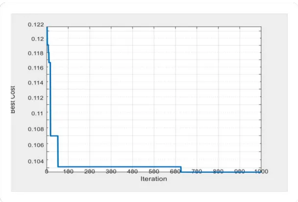
Figure 3.8: Example of convergence curve of best cost giving by ICA in each iteration from 0 to 1000
The best solution is the selected features by ICA algorithm, in each run of ANN 1000 iterations are done, the results is giving in the 1000 iterations with best cost (MSE value ) Figure16 (the result that has the lowest cost function (MSE) is taken as final result)
3.6 Using Particle swarm optimization PSO
In our work also Particle swarm optimization is also implemented to find a best solution for our problem which are the optimal features, the PSO algorithm works in the same way as ICA , However PSO has particles which moves around in the search-space where the solutions is located , our PSO tries to find a solution between it .The cost function of PSO was also built using ANN algorithm ,thus the selected solutions by PSO particles are sent to the cost function ,where the ANN is trained on them and then it calculates the MSE
value to compare the ANN output with the required target .then this value is returned back to the PSO in order to determine a new solution.
Figure 3.9: The way PSO works to select optimal features
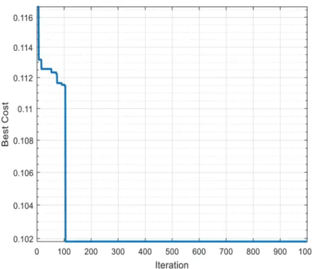
Figure 3.10: Example of convergence curve of best cost giving by PSO in each iteration from 0 to 1000
4. DECISION MAKING
There are two methods of classification technique in machine learning which are supervised and non-supervised methods, however in this part focus has been on the supervised method used in our work, therefore supervised classification is categorized into two as parametric and non-parametric methods.
In the supervised context we already have examples whose class is known and labeled. The data are therefore associated with class labels denoted Θ = {q1, q2, ..., qn}. The goal is then to learn using a learning model of the rules that allow to predict the class of new observations which amounts to determining a Cl function that from the descriptors (D) of the object associates a class qi and to also be able to affect any new observation to a class among the classes available. This comes back to the end to find a function we note Ys that associates each element of X with a Q element. then a template for classifying the new data. Among the supervised methods one quotes: k-nearest neighbors, decision trees, neural networks, machines with vector support (SVM).
Moreover, In this study Artificial neural network is used which is an example of nonparametric classifier. Non parametric classifiers are used in case of unknown density function and used to estimate the probability density function. Thus, there are large number of classifiers/methods come to existence that are used for classification task. Such as K- nearest Neighbor, Kernel Density Estimation, Artificial, Logistic Regression and neural network.
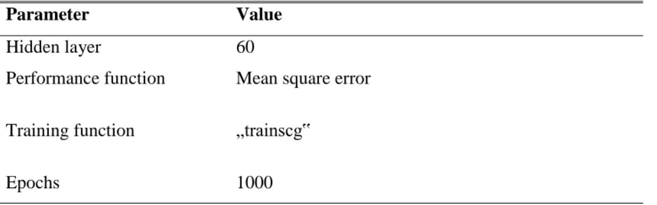
Hence the cascade forward neural network is implemented in this work ,which works as a cost function of one of optimization algorithm used ,60 number of hidden layer is used ,There can be multiple hidden layers in the model depending on the complexity of the function which is going to be mapped by the model. However, when there are many hidden layers, it takes a lot of time to train and adjust wights.More details about neural network used in this study are giving in Table 2.
Table 4.1: Parameters of ANN used in this work
Parameter Value
Hidden layer 60
Performance function Mean square error
Training function „trainscg‟
Epochs 1000
Using these settings illustrated in table 2 our proposed designed identified the optimal combination of features that will be used in detecting diseases under study.
4.1 Artificial neural network (ANN)
Neural networks are one of the most important fields of control engineering and artificial intelligence, which reflects a significant development in the human way of thinking. The idea of neural networks revolves around the simulations of the human mind using the computer.Artificial neural networks Are computational techniques designed to mimic the way the human brain performs a task by massively distributed parallel processing consisting of simple processing units. These units are computational elements called neurons or nodes, which have a neurological characteristic in that It stores practical knowledge and empirical information to make it available to the user by adjusting the weights.
The Artificial neural network (ANN) is similar to the human brain in that it acquires knowledge of training and stores this knowledge by using connecting forces within neurons called tangential weights.
Just as a human has input units that connect it to the outside world and its five senses, so do the neural networks, which need input units, and processing units where calculations are determined by the weights and through which the reaction is appropriate for each input of the network. Input units are a layer called the input layer, and the processing units are the processing layer that outputs the network outputs.
• Introduction of Neural network used in this work (feed forward) In this work cascade feed forward network is used, it is an acyclic artificial neural network, thus distinguishing itself from recurrent neural networks. The best known is the multilayer perceptron which is an extension of the first network of artificial neurons, the perceptron invented in 1957 by Frank Rosenblatt2.
• Artificial neural network in our work
The feed forward neural network was the first and simplest type of artificial neural network designed. In this network, information travels only in one direction, forward, from the input nodes, through the hidden layers (if any), and to the output nodes. There are no cycles or loops in the network.
Our Neural Network has Input which are the samples for the selected features (extracted features by ICA),and in the output has 5 classes which are the 4 diseases and healthy leaves ,Moreover the Algorithm used in this work is Imperialist competitive algorithm ,ICA‟s role is to suggest features from the extracted ones send it to cost function which send them to ANN and then it is trained on it and test the identified weights values with the samples set in order to calculate the value of the MSE ,this value will sent back to the cost function which will give it back to its agent to compare it with the latest value in order to update the cost value.
Figure 4.2: The proposed method of selecting optimal features
This systems works in the form of three connected rings between them it is role is to minimize the cost function, to determine the solution as shown in figure20,firstly ICA algorithm suggest random solution, sent to the cost function as selected solution where our ANN model is located .The ANN takes the samples of those selected features as input train on them using 60% (experiment 1) or 70% (experiment 2)of data After that the testing is done by ANN using 15% (experiment 1) or 20% (experiment 2) remaining data the MSE is calculated in order to compare the output with the required target .this operations is done in each run until the maximum iterations is reached .
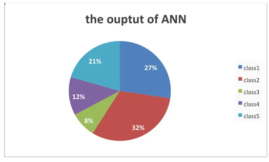
Figure 4.3: The percentage of samples in each class (The ANN‟s output) Our input will be classified according to 5 classes as shown in Figure 21, four classes are diseases images as explained before first class describes diseases called Alternaria Alternata which represents 21% of our datasets , from the second disease which is anthracnose 21% of images are manipulates, furthermore 8% of our data represents the third disease named Bacterial Bright , the forth class describes the Cercospora Leaf disease which is 12% ,in addition to those diseases extra class is included which is the class 5 (as shown in Figure 20) represents 32% of healthy leaves.
27 % 32 % 8 % 12 % % 21
the ouptut of ANN
class1 class2 class3 class4 class5
5. DESIGNED EXPERIMENTS AND RESULTS
5.1 Designed experiments
Forth experiments were conducted for the study of PSO and ICA algorithms in our work, according to the percentage of samples used in each experiment with both algorithms significant results were conducted which will be explained in details in the next section.
In order to collect enough results using two algorithms implemented in this study, two experiments are done for each algorithm operating the same datasets, as mentioned before both algorithm PSO and ICA have the same aim (finding optimal solution for optimization problem) However each in a different way .thus in this work 4 experiments are done, the number of samples has been changed according to testing, training and validation.
In each of these experiments approximately ten results are collected, the results obtained using artificial neural network in each run thus we have gathered around twenty different results for each algorithm.
Data sets used in this study:
RGB images with size of 256*256 pixels and four categories of diseases images are implemented; with healthy leaves. Total number of samples are used in the experiments is 73.
The features extracted from those images after segmentation and getting the region of interest represents the input of our neural network in each experiment, which the aim of our study is finding the optimal ones between them.
• Experiments of ICA algorithm Experiment 1:
In this experiment 20% of samples are used for validation 20% for testing and 60% for training, our proposed system try to find a solution to an optimization problem , the ICA algorithm is implemented to give the optimal features
between the nine features. The ICA suggests features from the giving ones by comparing between them using its own algorithm(explained before) the selected features is sent to the artificial neural network to test them ,at the same time it calculate the output and compare it with its target in order to get the MSE value (cost value). Furthermore, the error is calculated which will be sent back to the ICA as z-value, if this value is the lowest value founded it retains the features otherwise it looks for others this process is done until the ANN attend the maximum iterations which are 1000.
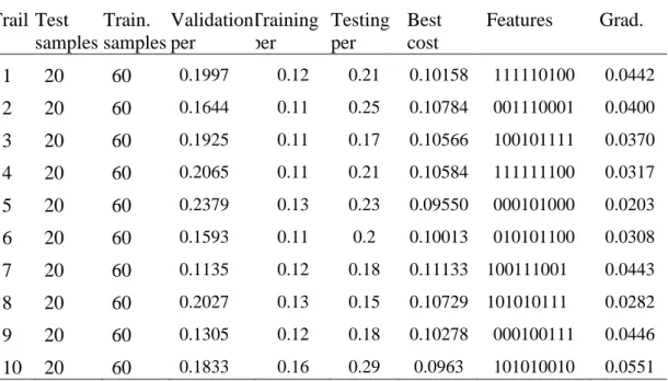
Table 5.1:10 trails done by ANN with ICA algorithm 20% testing 60% training and 20% validation. Trail Test samples Train. samples Validation per Training per Testing per Best cost Features Grad. 1 20 60 0.1997 0.12 0.21 0.10158 111110100 0.0442 2 20 60 0.1644 0.11 0.25 0.10784 001110001 0.0400 3 20 60 0.1925 0.11 0.17 0.10566 100101111 0.0370 4 20 60 0.2065 0.11 0.21 0.10584 111111100 0.0317 5 20 60 0.2379 0.13 0.23 0.09550 000101000 0.0203 6 20 60 0.1593 0.11 0.2 0.10013 010101100 0.0308 7 20 60 0.1135 0.12 0.18 0.11133 100111001 0.0443 8 20 60 0.2027 0.13 0.15 0.10729 101010111 0.0282 9 20 60 0.1305 0.12 0.18 0.10278 000100111 0.0446 10 20 60 0.1833 0.16 0.29 0.0963 101010010 0.0551 Table 3 contains results of ten trails done by our system with ICA algorithm, in each trail 20% samples for validation 60% samples for training and 20% testing are taken, as shown in the table different features and best cost are given in each of those trails also the gradient of error , Therefor in this experiment the testing performance in the eighth trail was the lowest one but according to validation it cannot be taken as a best results in this experiment. Moreover the testing performance of the trail 5 was approximately to the validation and also the cost value or MSE was the lowest one thus it can be taken as final result until all experiments being completed .
Graphics for each element are implemented in this experiment in order to see the extent of change in the pattern the graphics are as follows:
Figure 5.1: Validation performance of Experiment 1 by ICA in each trail In first experiment of ICA The maximum value of validation performance is shown in trail number 5 (0.12792) and the Minimum value was in trail 7 ( Figure) ,While the pattern was vibrated from the beginning until the end .
Figure 5.2: Training performance of Experiment 1 by ICA in each trail
The Figure 23 shows the values of training performance in experiment 1 of ICA which the high value was in trail 10 and the lowest one in trails 2,3 and 4 ,in addition to this the pattern of training performance in this experiment was also vibrated from the beginning until the end .
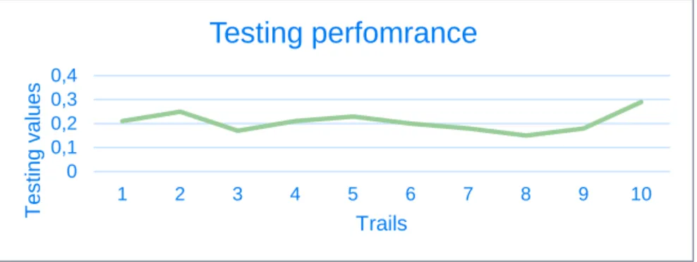
Figure 5.3: Testing performance of Experiment 1 by ICA in each trail
0 0,05 0,1 0,15 0,2 0,25 1 2 3 4 5 6 7 8 9 10 v al idat ion v al ues Trails
Validation performance
0 0,05 0,1 0,15 0,2 1 2 3 4 5 6 7 8 9 10 T rai ni ng v al ues TrailsTraining performance
0 0,1 0,2 0,3 0,4 1 2 3 4 5 6 7 8 9 10 T es ti ng v al ues TrailsTesting perfomrance
The figure 24 above shows the values of testing performance of experiment 1 which the pattern was vibrated and the maximum value was noticed in the last trail while the minimum one was in the trail number 8
Figure 5.4:: gradient of Experiment 1 by ICA in each trail
The pattern of gradient was also vibrated in this experiment as the figure shows, while the maximum value was in trail 10 and the minimum one was in trail 5 (figure 25) and we can also noticed that the gradient of error was very low in trail number 5.
Figure 5.5: The best cost of Experiment 1 by ICA in each trail
Figure 26 shows the pattern of last element of this experiment which is Best cost, while the maximum value was shown in Trail 7 and the lowest one was in trail5.
Experiment 2
In this experiment same algorithm is used ICA with ANN but with different percentage of samples, for validation 15% of samples is used ,70% for training and 15% for testing .our system work on the same way as mentioned before in
0 0,05 0,1 1 2 3 4 5 6 7 8 9 Gr ad ie nt v alu es Trails
Gradient
0,085 0,09 0,095 0,1 0,105 0,11 0,115 1 2 3 4 5 6 7 8 9 10 B es t c os t v al ues TrailsBest cost
the first experiment. The below table contains the results which will be explained in details below it.
Table 5.2: Nine trails done by ANN with ICA algorithm 15% testing 70% training and 15% validation
Trail Testing samples Train. Samples Validation per. Training per Testing per Best cost Features Gradient 1 15 70 0,38 0,15 0,3 0,0941 000111100 0,02928 2 15 70 0,1673 0,09 0,16 0,0803 001111100 0,03242 3 15 70 0,1331 0,12 0,28 0,1042 100000110 0,02544 4 15 70 0,254 0,25 0,5 0,1038 010111101 0,04678 5 15 70 0,1822 0,15 0,25 0,1075 101111000 0,0753 6 15 70 0,2303 0,15 0,2 0,1059 111110111 0,06047 7 15 70 0,2044 0,12 0,2 0,1078 101101001 0,0676 8 15 70 0,1638 0,12 0,163 0,1089 111010111 0,04948 9 15 70 0,1793 0,14 0,179 0,1046 001111110 0,0506
Table 4 shows results of experiment 2 the number of samples is changed ,each trails gives different results as in the first experiment but here we noticed that the lowest best cost was giving in trail number 1 but the testing and training error was high , However the result founded in trail 2 shows a lowest number of testing performance and also validation Moreover its cost function or best cost is lower according to the other ones ,Furthermore if we compare this result with the one in the experiment 1 ,this results is the best result or solution in both experiment because it has a lower cost function and testing performance
.
Figure 5.6: Validation performance of Experiment 2 by ICA in each trail
the validation performance of experiment 2 of ICA is shown on the (figure 27) above, which the pattern was also vibrated as in the first one, Moreover the maximum value was in first trail and the lowest one was in trail 3.
Figure 5.7: Training performance of Experiment 2 by ICA in each trail
The pattern of training performance of second experiment for ICA is shown in Figure As shown in the figure the performances vibrated from the beginning until the end but the high value was in trail 4 while the lowest one was in trail 2.
Figure 5.8: Testing performance of Experiment 2 by ICA in each trail.
0 0,1 0,2 0,3 0,4 1 2 3 4 5 6 7 8 9 V al idat ion v al ues Trails
validation performance
0 0,1 0,2 0,3 1 2 3 4 5 6 7 8 9 T ir ai ni ng v al ues Trailstraining performance
0 0,2 0,4 0,6 1 2 3 4 5 6 7 8 9 tes ti ng v al ues Trailstesting performance
Testing performance of this experiment was also vibrated as other elements while the maximum value was in trail 4 and the lowest one was in trail 2 as it is shown in figure 29 .
Figure 5.9: The gradient of Experiment 2 by ICA in each trail.
The figure 30 above shows the values of gradient of error in this experiment which the high value was in trail 7 and the lowest one in trail 5, Moreover the pattern was descending from the beginning trail until the fifth one after that it takes another turn however this pattern is also vibrated.
Figure 5.10: Gradient of Experiment 2 by ICA in each trail
This Figure 31 shows the best cost values giving in each trail which the high value was in trail 8 and the lowest one was in trail 1(0.0941) but as the testing error was high we have taken the result of trail number 2(0.10315) which has also a lower best cost and lowest testing error, however the pattern was oscillated from the beginning until the end.
0 0,02 0,04 0,06 0,08 0,1 0,12 1 2 3 4 5 6 7 8 9 bes t c os t v al ues Trails