τ χ
6 S 9 0 & э і ® 5 ш · е т ш ж тs s ï a i ï a x i 3?
j î i
İ
jc s î
C
â
İ («siK Ts w·” « .
1 Λ Ѵѵ \Ч “ :Л »Ч'і л f · ¿-ІЗзлЛ .л,S'UB'/îjTT£I î*>*" ■'“ іѵ.лс Г'h“ ’“.·.i C i t:' т г г т ’^'Л.г* *'" *
: 'V * Ï '3 ^ ѵ-.^’^ г А г 'і :>fíSZf ¿ . ·ί^·, :■ /5 ;j r,:„o,■.■ Λ.t! p^;■■ íO
5
^L*''£*-V '^·. ■:■ w^£?.5'lT/ ;■“■ ■ СГ “■ '■ ■ *-'f V.' К > C Г , '■ ^ ; D 'RADIUS OF CURVATURE AND LOCATION
ESTIMATION OF CYLINDRICAL OBJECTS WITH
SONAR USING A MULTI-SENSOR
CONFIGURATION
A TH ESIS S U B M IT T E D T O T H E D E P A R T M E N T O F E L E C T R IC A L A N D E L E C T R O N IC S E N G IN E E R IN G A N D T H E IN S T IT U T E O F E N G IN E E R IN G A N D SC IE N C E S O F B IL K E N T U N IV E R S IT Y IN P A R T IA L F U L F IL L M E N T OF T H E R E Q U IR E M E N T S F O R T H E D E G R E E O F M A S T E R O F S C IE N C E All Pcjolt.By
A ll Şafak Sekmen July 1997τ κ
^ 5 δΟ1 certify that I have read this thesis and that in rny opinion it is fully adequate, in scope and in quality, as a thesis for the degree of Master of Science.
Assist. Prof. Eh·. Billur Barshan(Supervisor)
I certify that I have read this thesis and that in my opinion it is fully adequate, in scope and in quality, as a thesis for the degree of Master of Science.
P rov Dr. Hayrettiii Köymen
I certify that I have read this thesis and that in my opinion it is fully adequate, in scope and in quality, as a thesis for the degree of Master· of Science.
/1
Assist. Prof. Dr. Orhan Ankan
Approved for the Institute of Engineering and Sciences:
Prof. Dr. Mehmet Bar ay y .
ABSTRACT
RADIUS OF CURVATURE AND LOCATION
ESTIMATION OF CYLINDRICAL OBJECTS WITH
SONAR USING A MULTI-SENSOR
CONFIGURATION
All Şafak Sekmen
M .S . in Electrical and Electronics Engineering Supervisor: Assist. Prof. Dr. Billur Barshaii
.July 1997
Despite their limitations, sonar sensors are very popular in time-of-flight measuring systems since they are inexpensive and convenient. One of the most important limitations of sonar is its low angular resolution. An adjustable multi-sonar configuration consisting of three transmitter/receiver ultrasonic transducers is used to improve the resolution. The radius of curvature es timation of cylindrical objects is accomplished with this configuration. Two different ways of rotating the transducers are considered. First, the sensors are rotated around their joints. Second, the sensors are rotated around their cen
ters. Also, two methods of tirne-of-flight estimation are implemented which are
thresholding and curve-fitting. Sensitivity analysis of the radius of curvature with respect to some important parameters is made. The bias-variance com binations of both estimators are compared to the Cramer-Rao lower bound. Theory and simulations are verified by experimental data from real sonar sys tems. Data is smoothed by extended Kalman filtering. Rotating around the center works better than rotating around the joint. Curve-fitting method is shown to be better than thresholding method both in the absence and pres ence of noise. The best results are obtained w'hen the sensors are rotated around their centers and the curve-fitting method is used to estimate the time- of-flight. There is about 30% improvement in the absence of noise and 50% improvement in the presence of noise.
ÖZET
Ç O K L U S O N A R D Ü Z E N L E Ş İM İ K U L L A N A R A K S İL İN D İR İK C İS İM L E R İN Y A R I Ç A P V E K O N U M
K E S T İR İM İ
A li Şafak Sekmen
Elektrik ve Elektronik Mühendisliği Bölüm ü Yüksek Lisans Tez Yöneticisi: Yrd. Doç. Dr. Billur Barshan
Tem m uz 1997
Ucuz ve kullanımlarının kolay olması nedeniyle, bazı sınırlamaları ol masına rağmen, sonar algılayıcılar uçuş zamanı ölçümlerinde çok sık kullanılmaktadırlar. Sahip oldukları sınırlamaların ilki düşük açısal çözünürlüktür. Bu çalışmada, çözünürlüğü arttırmak için, üç adet alıcı/verici ultrasonik sonar algılayıcıdan oluşan ayarlanabilir çoklu sonar düzenleşimi kul lanıldı. Bu düzenleşim ile silindirik cisimlerin yarıçap kestirimleri yapıldı. Algılayıcı döndürümünde iki yöntem kullanıldı. ilk olarak, algılayıcılar
askıları etrafında döndürüldüler, ikinci olarak algılayıcılar merkezleri etrafında
döndürüldüler. Ayrıca, uçuş zamanı kestiriminde de eşikleme ve eğri-uyarlama
yöntemleri uygulandı. Ayrıca kestiricilerin başarımmı saptamak için Cramer- Rao alt sınır karşılaştırması yapılmıştır. Analiz ve benzetim sonuçları, gerçek sonar sistemlerinden alman veriler kullanılarak desteklenmiştir. Genişletilmiş Kalman süzgeci ile veri düzleştirilmiştir. Algılayıcıların merkezleri etrafında döndürülmeleri daha iyi sonuç vermiştir. Eğri-uyarlama yönteminin eşikleme yönteminden daha iyi çalıştığı görülmüştür. Eğri-uyarlama yönteminin gürültüsüz bir ortamda yaklaşık %30 ve gürültülü bir ortamda yaklaşık %50 daha iyi sonuç verdiği gözlemlenmiştir.
ACKNOWLEDGMENTS
I am greatly thankful to my thesis advisor Dr. Billur Barshan for her super vision, guidance, suggestions and encouragement throughout the development of this thesis.
I would like to thank to my committee members Prof. Hayrettin Koymen and Dr. Orhan Arikan.
Special thanks to İlknur for her help and patience.
Many thanks to Birsel Ayrulu and M. Ertugrul Oner for their help and encouragement.
LIST OF SYM BO LS
Ртах propagation pressure
I'min minimum range
r range
./i(.) Bessel function of first order
a radius of the transducer
в deviation angle
Oo half beam-width angle
Л wavelength
pc reflection coefficient
Amax maximum amplitude
to time-of-flight /о resonant frequency
d transducer separation
hoi distance between the central transducer and the object
hii distance between the left transducer and the object
hri distance between the right transducer and the object
R radius of curvature
Го
1
range of the central transducerГЦ range of the left transducer
r,-i range of the right transducer
?’o
2
range of the central transducer after rotationri2 range of the left transducer after rotation
Гг2 range of the right transducer after rotation
a inclination angle of the left transducer
Г} inclination angle of the right transducer c the speed of sound
Ф rotation angle of the left transducer
¡5 rotation angle of the right transducer
R-2t III /(·) A i? Ahoi Ah-ri 4
n R )
'^1
bH0)Wo
W i tUr Zradius of curvature estimation after rotating the right sensor radius of curvature estimation after rotating the sensors radius of curvature estimate
perturbation on the radius perturbation on hoi
perturbation on hri
standard deviation of i? estimate bias of R estimate
standard deviation of r estimate bias of r estimate
standard deviation of 6 estimate bias of 9 estimate
noise on hoi
noise on hii
noise on hri
measurement vector
p{z\r, 0, R) conditional probability density function of z
x(A;) state vector z(A:) observation vector H(A:) Jacobian matrix
r maximum likelihood estimate of range
0 maximum likelihood estimate of angle
R maximum likelihood estimate of radius J Fisher information matrix
C error correlation matrix
Q
process noise correlation matrix R measurement noise correlation matrix P state covariance matrixP residual covariance matrix W filter gain matrix
TABLE OF CON TEN TS
1 INTRODUCTION
1
2 SONAR SENSING
4
2.1
Acoustic T ransducers...4
2.2 Tri-aural Sensor C onfiguration... 7
3 RADIUS OF CURVATURE ESTIMATION
9
3.1 Sensors Rotated around their Joints
9
3.1.1 Sensitivity Analysis of the Radius of Curvature Estimate 14
3
.1.2
Simulation R e s u l t s ... 153.2
Sensors Rotated around their C en ters...; . . . 293
.2.1
Simulation R e s u l t s ... 30 3.3 Curve-Fitting Method for Time-of-Flight Estimation 31 3.3.1 Simulation R e s u l t s ... 35 3.4 The Comparison of the Estimation Errors with the Cramer-RaoLower B o u n d ... 36 3.5 D iscu ssion ... 40
4 LOCATION AND RADIUS OF CURVATURE ESTIMA
TION
44
4.2 Simulation R e s u l t s ...
45
4.3 The Comparison of the Estimation Errors with the Cramer-Rao Lower B o u n d ... ...
55
5 SMOOTHING OF THE ESTIMATES USING EXTENDED
KALMAN FILTERING
60
5.1 A lg o r it h m ... ... 605.2 Simulation R e s u l t s ... 61
6 EXPERIMENTAL RESULTS
70
6.1
Experimental Set-up with Panasonic T ra n sd u cers... 706.2 Experimental R e s u lts... 72
6
.2.1
Thresholding M e th o d ... 726
.2.2
Curve-fitting M e t h o d ... 766.3 Experimental Set-up with Polaroid T ran sdu cers... 80
6.3.1 Experimental Results with the EKE SO 6.4 D iscu ssion ... ' . . . 82
7 CONCLUSION AND DIRECTIONS FOR FUTURE WORK 90
7.1 Summary of T h e s i s ... 907.2 Directions for Future W o r k ... 91
A CRAMÉR-RAO LOWER BOUNDS
92
B EXTENDED KALMAN FILTER ALGORITHM
96
C CHI-SQUARE DISTRIBUTED RANDOM VARIABLES
99
LIST OF FIGURES
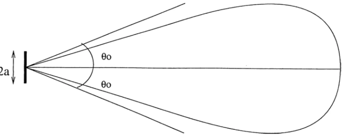
2.1
The main lobe of the radiation pattern of the Polaroid transducer.5
2.2
Cross-section of the Panasonic transducer...6
2.3 The tri-aural configuration where the sensors are aligned... 7 2.4 The beam patterns of the sensors (within dotted lines) iind their
sensitivity region (within solid lines)...
8
2.5 The tri-aural configuration where the peripheral sensors are ro tated around their joints...
8
3.1 The object and the tri-aural configuration...’ . . . 13
3.2 Noiseless and noisy signal models. 13
3.3 Sensitivity of R to distance measurements (a) hoi (fi) h,-i or hn
for d = 10 cm, i? = 5 cm and 9 = 0°... 16 3.4 Sensitivity of R to (a) d, (b) R and (c) 9 when Ahoi = 0.18 mm. 17 3.5 Sensitivity of R to (a) d, (b) R and (c) 9 when Ahri = 0.18 mm. 18 3.6 Estimated radius versus d, hoi iind noise standard deviation. . .
21
3.7 Estimated versus true radius for d = 15 cm, d = 20 cm, and d = 25 cm ... 22 3.8 Estimated radius versus d, hoi and noise standard deviation us
ing a
100
-iteration Monte Carlo simulation study... 23 3.9 Estimated versus true radius for d = 15 cm d = 20 cm andз л о Estimated radius versus d,hoi and 0 in the absence of noise. . . 25 3.11 Estimated versus true radius for d = 15 cm d =
20
cm andd = 25 cm in the absence of noise... 26
3.12
Estimated radius vei'sus d,ho\ and 0 in the presence of noise using a 100-iteration Monte Carlo simulation study... 27 3.13 Estimated versus time radius for d = 15 cm d = 20 cm in thepresence of noise using a 100-iteration Monte Carlo simulation
study. 28
3.14 The object and the sensor configuration when the sensors are rotated around their centers... 29 3.15 Estimated radius versus d,hoi and noise standard deviation
(when sensors are rotated around their centers)... 32 3.16 Estimated radius versus true radius when d = 20 cm and d = 40
cm (when sensors are rotated around their centers)... 33 3.17 Estimated radius versus d, hoi by using a
100
-iteration MonteCarlo simulation study... 33 3.18 Estimated radius versus true radius when d = 15 cm d = 20 cm
and d = 25 cm by using a
100
-iteration Monte Carlo simulationstudy. 34
3.19 Curve-fitting method to estimate the time-of-flight... 35 3.20 Estimated radius versus d and true radius when tirne-of-flight is
estimated by the curve-fitting method when sensors are rotated around their joints... ... 37 3.21 Estimated radius versus d, hoi ^.nd R when sensors are rotated
around their centers and the curve-fitting method is used in a noiseless environment... 38 3.22 Estimated radius versus d, hoi and R when sensor are ro
tated around their centers, the curve-fitting method and a
100
- iteration Monte-Carlo simulation study are used... 39 3.23 CRLB, bias, bias-variance combination versus d with (a),(b)3.24 CRLB, bias, bias-variance combination versus R with (a),(b) thresholding and (c),(d) curve-fitting methods... 3.25 CRLB, bias, bias-variance combination versus ho\ with (a),(b)
thresholding and (c),(d ) curve-fitting methods...
42
43
4.1 Location and radius of curvature estimation versus d in a noise less environment with the curve-fitting method when sensors are rotated around their centers (note that both estimates are the same)... 4.2 Location and radius of curvature estimation versus hoi in a noise
less environment with the curve-fitting method when sensors are rotated around their centers (note that both estimates are the same)... 4.3 Location and radius of curvature estimation versus R in a noise
less environment with the curve-fitting method when sensors are rotated around their centers (note that both estimates are the same)... 4.4 Location and radius of curvature estimation versus cl under
noise with the curve-fitting method when the sensors are rotated around their centers and a
100
-iteration Monte Carlo simulation study is employed...47
48
49
51 4.5 Location and radius of curvature estimation versus hoi under
noise with the curve-fitting method when the sensors are rotated around their centers and a 100-iteration Monte Carlo simulation study is employed... 52
4.6
Location and radius of curvature estimation versus R under noise with the curve-fitting method when the sensors are rotated around their centers and a100
-iteration Monte Carlo simulation study is employed... 53 4.7 Location and radius of curvature estimation versus 0 undernoise with the curve-fitting method when the sensors are rotated around their centers and a
100
-iteration Monte Carlo simulation study is employed... '544.8 CRLB versus d. First column is with thresholding and second column is with curve-fitting... 56 4.9 Bias, bias-variance combination, standard deviation versus d
with thresholding (first column) and curve-fitting methods (sec ond colum n)...
57
4.10 CRLB versus hoi. First column is with thresholding and second column is with curve-fitting... 58 4.11 Bias, bias-variance combination, standard deviation versus hoi
with thresholding (first column) and curve-fitting methods (sec ond colum n)... 59
5.1
Measurement residuals of Kalman filtering for d = 10 cm, R = bcm, hoi = 100 cm, ^ = 0°, measurement noise std = 10“ ® V, variance of radius noise =
10
“ ® cm®, variance of angle noise =10
“ '* rad®... 635.2
Estimated and predicted values of Kalman filtering lor d = 10 cm, R — b cm, hoi = 100 cm, 0 — 0°, measurement noise std = 10“ ® V, variance of radius noise =10
“ ® cm®, variance of anglenoise =
10
'* rad®. 645.3 Kalman filtering and estimates by one raw data sequence versus iteration numbers for d = 10 cm, R = b cm, hoi = 100 cm,
9 = 0°, measurement noise std = 10"® V, variance of radius noise = 10“ ® cm®, variance of angle noise = 10“ '* rad®. 65 5.4 Kalman filtered R, r, 9 versus d for true R = b cm, hoi = 100
cm, 9 = 0°, measurement noise std = 10“ ® V, variance of radius noise =
10
“ ® cm®, variance of angle noise =10
“ '* rad®, number of iterations = 25...66
5.5
Kalman filtered i?, r, 9 versus true R for d = 10 cm, hoi = 100cm, 9 = 0°, measurement noise std = 10“ ® V, variance of radius noise =
10
“ ® cm®, variance of angle noise =10
“ '* rcvd®, number of iterations = 25... 675.6 Kalman filtered R, r, 6 versus ho\ for R = 5 cm cl =
10
cm,6 = 0°, measurement noise stcl = 10“ ® V, variance of rciclius noise =
10
“ ® cm^, variance of angle noise =10
“ '‘ rad^, number of iterations = 25...68
5.7 Kalman filtered /?, r, 6 versus true 0 for i? =
5
cm d =10
cm,hoi = 100 cm, measurement noise std = 10“ ® V, variance of radius noise =
10
“ ® cm^, variance of angle noise =10
“ '^ rad^, number of iterations = 25... 696.1
The experimental set-up consisting of Panasonic transducers. . . 71 6.2 The block diagram of experimental set-up with Panasonic transducers... 71 6.3 Two extreme positions of the sensing device... 81 6.4 Measurement residuals of the Kalman filter for d = 7.5 cm,
R = b cm, hoi — 100 cm, 0 = 0°, vciriance of radius noise =
10
“ ® cm^, variance of angle noise =10
“ '’ rad^, initial estimatesR = b.l cm, hoi = 99 cm and ^ = 0.1°... 83 6.5 Estimates of the Kalman filter for d = 7.5 cm, R = b cm,
hoi -
100
cm, 0 =0
°, variance of radius noise =10
“ ® cm^, variance of angle noise = 10“ '’ rad^, initial estimates R = 5.1 cm, hoi — 99 cm and 0 = 0.1°... 846.6
Measurement residuals of the Kalman filter for d = 7.5 cm, i? =10
cm, hoi =100
cm, 0 =0
°, variance of radius noise =10
“ ® cm^, variance of angle noise =10
“ ^ rad®, initial estimatesR = 10.1 cm, hoi = 99 cm and 0 = 0.1°... 85 6.7 Estimated values of the Kalman filter for d = 7.5 cm, R = 10
cm, hoi =
100
cm, 0 =0
°, variance of radius noise =10
“ ® cm®, variance of angle noise = 10“ '’ rad®, initial estimates R = 10.1 cm, hoi = 99 cm and 0 = 0.1°...86
6.8
Measurement residuals of the Kalman filter lor cl = 7.5 cm,R = b cm, hoi = 140 cm, ^ = 0°, variance of radius noise =
10
“ ® cm®, variance of angle noise =10
“ '’ rad®, initial estimates6.9 Estimated values of the Kalman filter for cl = 7.5 cm, R = 5
cm, hoi = 140 cm, 6 = 0°, variance of radius noise = 10“ ^ cm^, variance of angle noise = 10“ '* rad^, initial estimates R = 5.1
cm, hoi = 139 cm and ^ = 0.1°...
6.10 Target discrimination using radius of curvature estimation. 89 88
LIST OF TABLES
6.1 Experimental results when ho\ = 500 mm, R = 75 mm, 0 = 0°
and the thresholding method is used...
73
6.2
Experimental results when hoi = 600 mm, R = 75 mm, = 0°and the thresholding method is used...
73
6.3 Experimental results when hoi = 500 mm, i? = 48 mm, 0 = 0°
and the thresholding method is used... 73 6.4 Experimental results when hoi — 600 mm, R = 48 mm, 0 = 0°
and the thresholding method is used... 74 6.5 Experimental results when hoi = 500 mm, R = 25 mm, 0 = 0·^
and the thresholding method is used... 74
6.6
Experimental results when the thresholding method is used to estimate the radius of curvature of a plane at hoi = 500 mm and ^ = 0°... 75 6.7 Experimental results when the thresholding method is used toestimate the radius of curvature of a plane at hoi = 600 mm and
0 = 0°... 75
6.8
Experimental results when the thresholding method is used to estimate the radius of curvature of a cylinder at hoi = 500 mm,d = 400 mm and R = 25 mm... 75
6.9 Experimental results when hoi = 500 mm, R = 75 mm, 0 = 0°
and the curve-fitting method is used...,77 6.10 Experimental results when hoi = 500 mm, R = 75 mm, 0 = 0°
6.11
Experimental results when hoi = 500 mm, i? = 48 mm, 0 = 0°and the curve-fitting method is used...
77
6.12
Experimental results when hoi — 600 mm, R = 48 mm, 0 = 0°and the curve-fitting method is used... 78 6.13 Experimental results when hoi = 500 mm, R = 25 mm, 0 = 0°
and the curve-fitting method is used. ... 78 6.14 Experimental results when the curve-fitting method is used to
estimate the radius of curvature of a plane at hoi = 500 mm and ^ = 0°... 79 6.15 Experimental results when the curve-fitting method is used to
estimate the radius of curvature of a plane at hoi = 600 mm and ^ = 0°... 79 6.16 Experimental results when the curve-fitting method is used to
estimate the radius of curvature of a cylinder at hoi = 500 mm,
Chapter 1
INTRODUCTION
Ultrasonic sensors are a convenient and inexpensive means for a mobile robot to build a model of its environment. However, these sensors have some limitations such as high beam-width which makes it difficult to localize objects correctly, and multiple reflections which may be difficult to interpret. In order to decrease the effect of these limitations, an adaptive multi-sensor configuration is used, composed of three transmitter/receiver ultrasonic transducers. This way, the radius of curvature and location of the reflecting object can be estimated. With the estimation of the radius of curvature, different types of reflectors such as walls, cylinders and edges can be discriminated. For large values of radius, the object can be assumed to be a planar wall, and for values close to zero, the object can be assumed to be an edge [
1
].Barshan and Kuc differentiated sonar reflections from corners and planes by using a multi-transducer sensing system [
2
]. Kuc used a system which adaptively changes its position and configuration in response to the echoes it detects [3]. In [4], Kleeman and Kuc classified the target primitives as plane, corner, edge and unknown, and showed that in order to distinguish these, two receivers and two transmitters are necessary and sufficient in a non-adaptive configuration. In [5], Sasaki and Takano showed that the echo signals from the same object in different locations may have more variation than that from different objects. In order to decrease the limitations of sonar, Flynn used a multi-sensor configuration consisting of infrared and sonar sen sors [6
]. In [7,8
, 9], acoustic sensors were used for sonar mapping. Ohya and Yuta investigated how the information obtained by the ultrasonic sensor is affected by the characteristics of the sensing systems such as sensitivity and directivity [10
]. In [11
], Sabatini illustrated that advanced filtering methodsare required for making data more accurate and reliable. He also proposed a digital-signal-processing technique for building a transducer array capable of automatically compensating for variations in the speed of sound due to tem perature or any other atmospheric conditions [
12
]. Curran and Kyriakopoulos used an extended Kalman filter to combine dead-reckoning, ultrasonic, and inlrared sensor data to estimate current position and orientation of a mobile robot [13]. Webb, Gibson and Wykes used novel sensors to measure the range and bearing of a target and guide the robot [14]. In [15, 16,17], acoustic sensors were used for robot navigation. In [18], Ko, Kim, and Chung used sensors to extract multiple landmarks for the indoor navigation of a mobile robot. Chang and Song solved the beam-opening angle problem by fusing data from multiple ultra.sonic sensors [19]. In [20, 21, 22], a sensor with the flexibility to track 3-D targets which are not necessarily in the same horizontal plane as the sensors is investigated. Moreover, radius of curvature estimation is important in image analysis to provide viewpoint-independent cues for shape classification [23].In this thesis, the work done in [
1
] and [24] is extended to an adaptive tri-aural sensor for improved radius of curvature and location estimations of targets. When the object and the sensor are not perpendicular to each other, there is an exponential decline in the amplitude of the reflected sonar signal which decreases the signal-to-noise ratio. In order to avoid this problem, an adaptive tri-aural sensor is developed. Depending on the location of the object, the sensor can rotate its transducers to get a more accurate radius of curvature estimation. First, a tri-aural sensor composed of three sensors is employed. According to the measurements made with this set-up, the peripheral sensors are rotated around the joints. Also, the case in which the sensors are rotated around the centers is investigated.In Chapter
2
, background information on sonar sensors is given. The main reason why the sonar sensors are rotated is discussed. Also, rotated configura tions of the sonar sensors are illustrated.In Chapter 3, radius of curvature estimation is described. In order to es timate the time-of-flight values, two different methods are used. First, the traditional thresholding method is tested which is fast but biased and sub- optimal. Second, the curve-fitting method which is slower but more accurate compared to the thresholding method is used. The sensitivity of estimation to the distance between sensors, the true radius, cind the range is investigated. In Section 3.1, the case in which the sensors are rotated around their joints is investigated. In Section 3.1.1, the sensitivity analysis of the radius of curvature is performed. In Section
3
.2
, the case in which the sensors are rotated aroundtheir centers is investigated. Noiseless and noisy cases are studied separately. In order to obtain reliable results in a noisy environment, a 100-iteration Monte Carlo simulation study is performed. In Section 3.3, the curve-fitting method is described. In Section 3.4, in order to evaluate the estimation performance, a comparison with the Cramer-Rao lower bound is made.
In Chapter 4, the radius of curvatiu'e estimation is extended to location estimation.
In Chapter 5, an extended Kalman filter is used to estimate the radius of curvature and location of cylindrical objects.
In Chapter
6
, the experimental results of both thresholding and curve-fitting methods are presented.In Chapter 7, conclusions are drawn and directions for future work are motivated.
In Appendix A, the details of the Cramer-Rao lower bound calculation are given. In Appendix B, the model for the extended Kalman Filter which is used to estimate location and radius of curvature of cylindrical objects is detailed. In Appendix C, the properties of chi-sciuare distributed random variables are presented. In Appendix D, the computer programs with which the simulations are performed and the experimental results are analyzed are presented.
Chapter 2
SONAR SENSING
In this chapter, some properties of sonar sensing are discussed. The multi-sonar configuration is introduced and the reasons why this configuration is used are given.
2.1
Acoustic Transducers
Ultrasonic transducers are acoustic devices having a resonant frequency higher than 20 kHz. They have been used widely in burglar ahirm systems, proximity switches, anti-collision devices, counter for moving objects and T V remote control systems. Since the characteristics of the sound produced by an acoustic transducer change with distance, the near-held region (the neighborhood of the transducer) and the far-held region (beyond the near-held) are investigated separately. The near-held region is called as Fresnel diffraction zone and the far-held region is called as Fraunhofer zone [25]. The expression for the sound pressure within the near-held is relatively complex, and not in the scope of this thesis. The far-held characteristics at range r cind angular deviation 0 for a
single frequency of excitation is described by [26, 27]
A(r,0) = Pn Ji{kasm 0)
ka sin 0 for > r.
(
2
.
1
)
where Ji(·) is the Bessel function of hrst order, and Pmax is the propagation pressure amplitude on the beam axis at range rmin along the line-of-sight.
The half beam-width 0o in the far-held region corresponds to the hrst zero of the Bessel function in Equation 2.1 which occurs at ka sin 0 = 1.227T and the
Figure 2.1: The main lobe of the radiation pattern of the Polaroid transducer.
following equation is obtained for the half beam-width angle [28]: "o.eiA'
6o = sin ^
a
(2.2)
where A = c / / is the wavelength, and a is the radius of the transducer.^ The radiation pattern is shown in Figure 2.1.
Since a range of frequencies around /o are transmitted, the correspond ing beam patterns are superposed and the resulting beam pattern can be ap proximated by a Gaussian beam profile centered around zero with standard deviation erg = ^ [16, 27]:
A (r, 9) = ■ 'm a x · m i n--- e e for
r > r
_ · m i n (2.3)Since the position and radius of curvature of cylindrical objects are going to be estimated, a reflected sonar signal model for cylindrical objects is needed. The signal model is basically a sinusoidal enveloped by a Gaussian which is given by [27, 29]:
3 /2
m a x ' m i n ^ ,2
sin [27r/o(i - to)] (2.4) where pc is the reflection coefficient depending on the radius of curvature (for r > 5 cm, pc — 0.0044946/7 — 0.0022471 [29]), A-max is the maximum amplitude,
7
’ is the distance between the sensor and the center of the object, r^in — «^/A (a is the radius of the transducer aperture, 0.65 cm for the Panasonic and 2cm for the Polaroid), 0 is the angle normal to the receiver with respect to the object, ae = ^o
/2
(0o is the half beam-width angle), to is the time-of-flight, fois the resonant frequency (49.4 kHz for Polaroid, 40 kHz for Panasonic), and
(^t = l / / o .
The cross-section of the Panasonic transducer is pictiired in Figure
2
.2
.Internal Construction
_ C o firuîctor AlufTiinum Resonator Lead W ire Pi(;/0(îl<îciric Ceram ic ElernenrTerm inal Pin .
2.2
Tri-aural Sensor Configuration
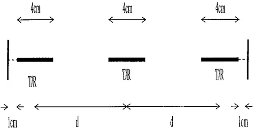
In this study, a tri-aural sensor composed of three sensors was employed as shown in Figure 2.3. Each one of the transducers is sensitive to echo signals reflected within its beam pattern. The actual beam pattern is similar to the region illuminated by a flashlight. All members of the tri-aural configuration can detect targets located within the overlap of the three becim patterns, which is called the sensitivity region^ as illustrated in Figure 2.4. In fact, the bound aries of the sensitivity region change with the type of object. For example, for edge-like or pole-like targets, this region is much smaller but of similar shape, and for planes, it is more extended.
t a
<--- >
t a--- >
t a<--->
1
^
Icoi kmFigure 2.3: The tri-aural configuration where the sensors are aligned. As seen from Equation 2.4, when the object and the sensor a.re not perpen dicular to each other {6 ^
0
°), there is an exponential decline in the amplitude which decreases the signal-to-noise ratio. Hence, information provided by sonar sensors is most reliable when the object is perpendicular to the sensor, and at nearby ranges due to the term in Equation 2.4. Because of this, the transducers are rotated to make them orthogonal to the object. In this study, two methods to rotate the transducers are used. First, the sensors are rotated around their joints as shown in Figure 2.5. Second, the sensors are rotated around their centers as will be shown later in Figure 3.14.Figure 2.4: The beam patterns of the sensors (within dotted lines) and their sensitivity region (within solid lines).
4cra/
T/R
4cm
<--->
T/R
Figure 2.5: The tri-aural configuration where the peripheral sensors are rotated around their joints.
Chapter 3
RADIUS OF CURVATURE
ESTIMATION
In this chaptei', radius of curvature estimation of cylindrical objects is de scribed. Two different ways of rotating the sensors are investigated. Two methods are used in order to estimate the time-of-flight. Sensitivity analysis for radius of curvature estimation is performed. Finally, the performances of the estimators are compared to the Cramer-Rao lower bound.
3.1
Sensors Rotated around their Joints
Figure 3.1 illustrates the object and the tri-aural configuration.
As seen from Equation 2.4, in order to model the sonar signal, the time-of- flight information is needed.
The following algorithm describes how the sensors can be rotated with respect to the target location in the simulations:
• Take the true values of hoi,R.,d and 0.
• The true distances between left transducer and the surface of the ob ject and right transducer and the surface of the object (Ari) fii’e
computed from the geometry:
K i = \Ji’oi + (P - 2f/roi sin 0 — R
hii = + 2droi sin 0 - R (3.1)
• The distances of the three sensors to the center of the object and their inclination angles are calculated:
r;i — hii R f'oi — ho\ + R — ^^7*1 I R^ (3.2) U = Sin 2dr
ol
2drn T] = sin- 1 (3.3)• The signal from each sensor is modeled by finding the time-of-flight val ues corresponding to hoi, hn and
hri-• For the central sensor: For the left sensor: For the right sensor:
-- , normal angle = 0.
toi = , normal angle = a;. , normal angle = r/.
2hr.
c
2h.
tor -- 2hri
• The signals are modeled according to Equation 2.4 by using the time-of- flights obtained. The following model parameter values are used:
■‘^max
~1
CnClI'min
10
cmPo = 0.44946i? - 0.022471 /o = 50 kHz
c = 34350 cm /s
• White Gaussian noise W (0, cr) is added to the signal at every 1 p s and the noisy signal model is obtained.
The noiseless and noisy signal examples are shown in Figure
3
.2
(a) and (b) respectively.• The time-of-flight can be estimated by choosing an appropriate thresh old. In this case, the threshold is chosen as 5a and the first time instant where the noisy signal exceeds the thresholding is detected. This is the noisy tirne-of-flight estimate, h — is used to find the noisy hoi, hn
and
hri-• By using the noisy hoi,hn and hri, the initial estimates of 0 ,a and r]
values are calculated, and the radius of curvature is estimated from the measurements:
(^ri + ^n) ~ ^{^li +
Ri =
(3.4)4/i.oi — 2(/iri + hii)
• The noi.sy distance of the left sensor is estimated and the rotation angle is calculated accordingly:
ri2 = y/7'fi +
6
r/i sin a a = Z i = r2
_ r-2
^12 'll b =6
-h 2r¡i sin Q' 2ri2 S — ab \/a2 — 6ab + 9 2 r i 2 6 2 - 1 6 2 - 1 / - 1/ 3
(j) = cos zi 3 (3.5)The left sensor is rotated by (/>.
After the left sensor is rotated, the radius of curvature is estimated again: Cl = ^(^, + 3 ) 2 - 3 2 hl2 - ri2 - Ri C2 = hi2 — Cl C
3
= d - Zi R21 — cl — 62j -f C3
—2
C2
C3
sin (f> 2hoi - 2c2 +2
c3
sin (j) (3.6)• The noisy distance of the right sensor is estimated and the rotation angle is calculated:
a = Zr =
K
2
-
b =6
+ 2rri sin a2
r 7-22
r,.2
S — ab Vo^ — 6ab + 9 /5 = cos62-1
- 162-1
+ 3 (3.7)• After rotating the right sensor by /3, the radius of curvature is estimated again: C
4
- y/{zr + 3 y -32
hr2 — ^V2
“ C5
hj'‘2 C4
Cq — cl Zj· c l - h l^ + c l - 2C5C6 sin /? Rot --2h o i — 2c5 + 2ce sin ^ (3.8)• The average of the radius values calculated by rotating the left and right sensors are calculated:
Figure 3.1: The object and the tri-aural configuration.
Noiseless Sonar Signal Model Noisy Sonar Signal Model
(a) (
6
)3.1.1
Sensitivity Analysis of the Radius of Curvature
Estimate
In this section, the sensitivity analysis of the radius of curvature estimation to parameters such as hoi·, hn, h^i, cl, R and 0 is presented. The sensitivity amilysis can be summarized by the following steps:
• Function / ( . ) for the radius of curvature estimate is defined as follows;
f(h hi h d) - B - (^ri + hfi) - 2{hl-^ + cP)
i{h o i,h n ,K i,d ) - R i - (.3.10)
• Perturbation is added to the variable for which sensitivity analysis is made. For example, the perturbation Ahoi is added to
hoi-• The perturbation on radius of curvature is calculated as follows:
i^ri T ~ 2[(/ioi + AhoiY + d^]
fihoı-l·Ahoı, hii, hri, d) — + —
4(/ioi + Ahoi) — 2(/iri + hii)
(3.11) • The effect of the perturbation on the radius of curvature estimate is
found:
A R — fi^hoi T Ahoi, hn, h^i, d^ f ijioi, hn, h^i, d^ (.3.12)
Figure 3.3(a) is plotted for hoi between 0-150 cm. The error in hoi is positive and between 0-0.4 mm. A stationary cylindrical target at 0 = 0° with radius 5 cm is used and transducer separation is assumed to be 10 cm. The error A R in R increases linearly with the error Ahoi and nonlinearly with hoi-
Also a positive error in hoi leads to a positive error in R since for constant
hri and hii, increasing hgi means increasing R, as the geometry of Figure 3.1 indicates. As range increases, the error also increases since the sensor has lower resolution for fixed d.
In Figure 3.3(b), the same parameters are used as in Figure 3.3(a) with a positive error in hri instead of hoi- Since the terms h,.i and hn are used symmetrically in the radius of curvature equation, the sensitivity analysis of
¡Hi gives the same results. A positive error in h^i or hn causes a negative error in R since a positive error on left and right measurements for constant central sensor measurement leads to a reduction in R as in Figure 3.1.
Figure 3.4(a) and 3.5(a) show the effect of d on the radius of curvature estimation. Ahoi = Ahri = 0.18 mm errors are taken for Figure 3.4(a) and 3.5(a) respectively. Range is again varied between 0-150 cm. The error is plotted for d between 4-40 cm. As seen from the figures, for small d/ho), the error is high since the resolution of the left and right sensors decrease as shown in Figure 2.4. Hence, as range increases the transducer separation should also be increased to achieve higher resolution. Also for high values of d/hoi, the error is large since the sensitivity patterns of the transducers will not overlap at the target [30].
Figures 3.4(b),(c) and 3.5(b),(c) illustrate the sensitivity of radius of cur vature to measurement errors Ahoi = 0.18 mm and Ah,.i = 0.18 mm, re spectively. In Figures 3.4(c) and 3.5(c), 0 is varied from 0° to 20° with 1° increments.
3.1.2
Simulation Results
Now, the simulation results can be investigated by using the results of the sensitivity analysis.
Figure 3.6-3.9 show the simulation results for 0 = 0°.
Figure 3.6 and 3.7 show how the estimated radius values Ri aild i
?2
are affected from different variables in the absence of noise. Figure 3.8 and 3.9 show the same calculations obtained with the Monte Carlo simulation study.The sensitivity analysis of the calculated radius of Equation 3.4 to
hoi, hn, hri,d and R shows that the radius is very sensitive to these variables. A positive error in hoi (A/ioi > 0) causes the estimated radius to be greater than the true radius (according to Equation 3.4). A positive error in hu or /i^i
(Ahii > 0) causes the estimated radius to be less than the true radius. More over, the error corresponding to the separation between the sensors is positive and it decreases as the separation increases. As the distance between the sen sors and the object increases, the error increases in the negative direction.
The results are completely consistent with the sensitivity analysis predic tions. Although the noise is zero in some cases, the estimated radius deviates from the true radius. The error sources are the bias error due to thresholding and the error due to sampling the signal.
h (cm)
(a)
h ,(cm)
ib)
Figure 3.3: Sensitivity of R to distance measurements (a) hoi (b) K i or hn for
(a) E t . ... ... ' ib) ( c)
(a)
(b)
( c )
Figure 3.6(a) shows the relation of the estimated radius and the se
2
Daration distance between the transducers. The error in the estimated radius values decreases as the separation increases. As stated previously, a ¡Dositive error inhot makes the estimated radius greater than the true radius, and a positive error in hit or hrt makes the estimated radius less than the true radius. Since there is error not only in hot but also in hit and hrt in this estimation, error is positive for some values of d and negative for some other values of d. Figure 3.6(b) shows the effect of hot on the estimated radius. As hot increases the error in the negative direction increases (that is, the error in hot is negative, A/ioi < 0). The estimated radius after rotating the left sensor is very close to the estimated radius of the linear configuration. Figure 3.6(c) shows the effect of the noise standard deviation on the estimated radius. In the presence of noise, the error after rotation is nearly the same as the error before rotation. However, for some values of the noise standard deviation (2xl0~® to 3x10“ '^ V ), it is greater than that of the linear case.
Figure 3.7 shows the effect of d and the true radius R on the estimated radius. At fixed distance, as R increases the error increases, and as d increases the error on the radius estimate decreases.
Figures 3.8 and 3.9 display the results of a 100-iteration Monte Carlo sim ulation study. In the figures, the effect of noise on d, hot and R is shown. The dashed line shows the mean value and the other two lines indicate one standard deviation from the mean. When Figure 3.6(a) and 3.8(a) are compared, the effect of noise on d can be observed. The estimated radius is less than the true radius for all values of d. This is because the negative error in hit a.nd hrt is more dominant than the positive error in hot- Figure 3.8(b) shows the effect of
hot and Figure 3.8(c) shows the effect of the noise standard deviation on the estimated radius.
Figure 3.9 shows the effect of d and R over a 100-iteration Monte Carlo simulation study. As the separation between the sensors increases, the standard deviation decreases. For low values of R and high values of d, the error is large since for large values of d the normal angle between the object and the left sensor increases, causing a high exponential decline in Equation 2.4.
Figures 3.10 and 3.11 illustrate the results o[ 0 ^ 0° case in the absence of noise. In Figure 3.10(a), the dependence of the estimated radius to the separation distance between the transducers is illustrated. As d increases, the error in the estimation of the radius of curvature corresponding to the linear configuration of the sensors decreases. Although the error in estimation after
rotating the sensors is larger than that of the linear configuration case, it decreases with d. After a certain value of d (around d = 27 cm), the error for both cases begins increasing since at that point, the target is not within the beam pattern of the left or right sensor. Figure 3.10(b) shows the effect of hoi
on the estimation of the radius of curvature. As hoi increases the error in both linear and rotated configurations increases. Figure 3.10(c) shows the effect of 0
on the estimated radius. As 0 increases, the error increases as expected, since a sonar sensor can make more accurate measurements along its line-of-sight. This is because the echo amplitude decreases exponenticilly with the square of
0 according to Equation 2.4.
Figure 3.11 shows the effect of d and true radius R on the curvature es timation. As d increases, the estimation error corresponding to the linear configuration decreases according to the sensitivity analysis but the error for the rotated configuration increases. This is because as d increases, the object goes out of the sensitivity region and the rotation angle calculated by using the linear configuration is not correct.
Figures 3.12 and 3.13 show the effect of noise on the above observations. In these figures, a 100-iteration Monte Carlo study was employed. Figure 3.12(a) shows the effect of d. In both cases, as d increases, initially the error decreases, and after a certain value of d (around d = 16 cm) the error increases sub stantially. Figure 3.12(b) shows the effect of hoi and Figure 3.12(c) shows the effect of 6. When Figures 3.10 and 3.12 are compared, the effect of noise can be observed. Figure 3.13 shows the effect of d and R. in the presence of noise. As d increases the estimates are degraded.
(a)
R eaScm d = s 1 0 c m ^ J o is o = 0 A v e r a g e R 1 **5.1 1 c m A v e r a g e R 2**S. 1 3 c m
(b)
R =*5cm d —1 O cm h 0 1 * * 1 0 0 c m
(c)
d=15cm ho1»a100cm Noise=0 (a) d=20cm ho1=100cm Noisei=0 (b) d=525cm ho1=100cm Noiso=0 (c)
Figure 3.7: Estimated versus true radius for d = 1.5 cm, d = 20 cm, and d = 25 cm.
(a)
R«5cm d=»15cm Noise Std=»5e—7 volt Average R1 «=4^.51 cm Average R 2=4.50cm
(b)
R=5cm d=10cm ho1—100cm Average R1 =4.51 cm Average R 2=4.50cm
(^)
Figure 3.8: Estimated radius versus d, hoi «'■nd noise standard deviation using a 100-iteration Monte Carlo simulation study.
d=15cm ho1=100cm Noise Std=»1 e - 6 volt
(a)
d=*20om ho1«»100cm Noise Std«*1 e —S volt
d»a25cm ho1=100cm Noise Std=1 e —6 volt
(c)
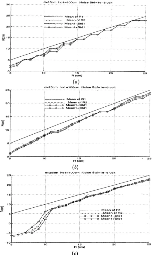
Figure 3.9: Estimated versus true radius for d = 15 cm d = 20 cm and d = 25 cm using a 100-iteration Monte Carlo simulation study.
(a)
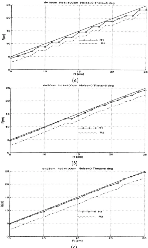
R*s5cm da*10cm Noise=0 Theta=5 deg
(b)
R*.5cm d=10cm ho1—100cm Noise^O
(c)
(a)
d=20cm ho1*x100cm Noise«0 Theta=5 deg
ib)
d=25cm ho1»100cm Nolse™0 Theta=«5 deg
(c)
Figure 3.11: Estimated versus true radius for d = 15 cm d = 20 cm and d = 25 cm in the absence of noise.
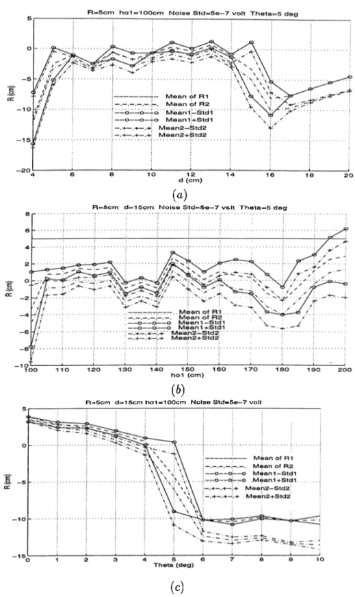
(a)
R*x5cm d=15cm Noise S td=5e—7 vcit Theta=s5 dog
(b)
R=5cm d=i1 5cm ho1*=100cm Noise Std=5o-7 volt
(c)
Figure 3.12: Estimated radius versus d, hoi and 6 in the ¡presence of noise using a 100-iteration Monte Carlo simulation study.
d=3l5cm ho1=100cm Noise Std=:5o—7 volt Theta=5 dog
(a)
d=20cm ho1**100cm Noise Std=5o—7 volt Thota=5 deg
(b)
p'igure 3.13: Estimated versus true radius for cl = 15 cm d = 20 cm in the presence of noise using a 100-iteration Monte Carlo simulation study.
3.2
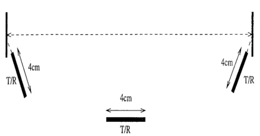
Sensors Rotated around their Centers
111
this part, we consider the case in which the left and right sensors are assumed to rotate around their centers as shown in Figure 3.14.Figure 3.14: The object and the sensor configuration when the sensors are rotated around their centers.
The algorithm to find the rotation angle can be summarized as follows:
• The initial estimate of the radius of curvature (when the sensors are aligned) is the same as in the previous algorithm.
• From the first set of measurements, noisy 0, a and r) are calculated:
9 = sin ^( r l - r l - d ^ \ 2clroi a = sin“ ^ r l - r l , + d ^ · V ^drn f ^rl - ?’oi + r¡ = sm 1 i 2i/r,.i (3.13)
• After finding the rotation angles, 0, a and r¡, the central, right and left transducers are rotated by 9, a and r¡ respectively. When the sensors are rotated, they are assumed to be perpendicular to the center of the object.
The nominal values of the distances after rotation should be:
^o2 —
hi2 = hn
hj-2 — hj-i (3.14)
• New measurements are taken and the second estimation of the radius of curvature is made by using Equation 3.4.
3.2.1
Simulation Results
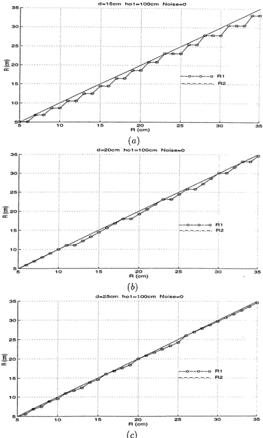
Figure 3.15 shows the effects of d, hot and noise standard deviation on the estimation of the radius of curvature when ^ = 0°. It can be seen that for all values of d, hot and noise standard deviation, the second estimation (after rotation) provides better results. Figure 3.15(a) shows that the deviation be tween the two estimates begin after a certain point in d (around d = 37 cm). Up to that point, the first and the second estimates are nearly the same since for low values of d, the normal angle of the left sensor is small and the object is nearly perpendicular to the left sensor. However, as d increases the normal angle of the left sensor also increases and the estimation after rotation provides improved results. Figure 3.15(b) shows that as hot increases, the first and sec ond estimates become closer. This is because when hot is small, the deviation angle of the left sensor is large and the estimation after rotation gives improved results. Figure 3.15(c) shows the effect of the noise standard deviation. The second estimation is less affected from noise than the first estimation.
Figure 3.16 shows the effect of d and R simultaneously. As d increases both estimators improve and for the low values of R the second estimation is more accurate for the same reason as above. For lower values of 72 (77 < 10 cm) and high values of d, the estimated radius after rotation is better since for high values of d, exponential decline in Equation 2.4 is very high.
Figures 3.17 and 3.18 show the same calculations done by using a 100- iteration Monte Carlo simulation study. Figure 3.17 shows the effect of d and
hot on the estimated radius in the presence of noise. Figure 3.17(a) indicates that as d increases, the second estimation provides better results which is con sistent with the above argument. When d is small, the object can be consid ered perpendicular to the sensors, hence we do not expect much improvement with the second estimation. Since there is error in the rotation angle, the es timation after rotation must be worse than that of the linear configuration.
Figure 3.17(b) shows that as hoi increases the first estimate improves since the object becomes perpendicular to the sensors.
Figure 3.18 shows the effect of d and R simultaneously on the radius of curvature estimation. As d increases, the second estimation improves as ex pected. For low values of R, as d increases the error in the first estimation also increases since for high values of d and low values of R, the normal angle of the left and right sensors are high and the exponential decline in Equation 2.4 is high.
3.3
Curve-Fitting Method for Time-of-Flight
Estimation
A curve-fitting approach is used in order to reduce the error in the time-of- flight estimations obtained from the thresholding method and improve the estimation procedure. Earlier, in [24], a similar method was used to improve the accuracy of point-target localization. It was shown that this method of time-of-flight estimation eliminated the bias resulted from thresholding and was comparable to thresholding in variance. Here, we generalize the method to include radius of curvature estimation. Figure 3.19 shows the parabola fitted noisy sonar signal model. It is expected to reduce the bias with this· method.
The following algorithm is used when estimating the time-of-flight with curve fitting:
• An approximate time-of-flight estimate is obtained using the thresholding method.
• The amplitude o f the signal is sampled at three time instants before the time-of-flight obtained by the thresholding method. The time interval between the time instants equals 3 ¡.is. •
• The zero-crossing parabola passing through these points is found. Parabola is assumed to be of the form y = at^ + bt + c, and the co efficients a, b and c are calculated by using the three samples. If the parabola found by using the above samples does not take the value zero at any time, then new samples are taken and another parabola is ob tained. This procedure continues until a zero-crossing parabola is found.
(«)
RaaScm d»1 Ocm Noise«0 Average R1 »:4.83cm Average R 2=5.02cm
(&)
R=5cmd=x10cm ho1=100cm Average R1 *=3.19cm Average R2=3.S7’cm
(c)
Figure 3.15: Estimated radius versus d, hoi «'•nd noise standard deviation (when sensors are rotated around their centers).
d=20cm ho1=100cm Noise=0 d=40cm ho 1=100cm Noise=0
(a) (b)
Figure 3.16: Estimated radius versus true radius when d = 20 cm and d = 40 cm (when sensors are rotated around their centers).
R=5cm ho1=100cm Noise S td=1e-6 volt R=5cm d=10cm Noise S td=1e-6 volt
(a) (b)
Figure 3.17: Estimated radius versus d,hoi by using a 100-iteration Monte Carlo simulation study.
(a)
d=20cm ho1=*100cm Noise Std=1 e—S volt
(b)
d»25cm ho1=x100cm Noise Std*1 e —6 volt
(c)
Figure 3.18: Estimated radius versus true radius when d = 15 cm d = 20 cm and d = 25 cm by using a 100-iteration Monte Carlo simulation study.
Figure 3.19: Curve-fitting method to estimate the time-of-flight.
• The time instant at which the value of this parabola is zero is the estimate of time-of-flight with the curve-fitting method.
3.3.1
Simulation Results
Figure 3.20 shows the results found by curve-fitting for 0 = 0° case when the sensors are rotated around their joints. The improvement in the results is about 40% with respect to the thresholding method.
Figure 3.20 shows the effect of d for two different noise levels. When Fig ure 3.20(a) is compared with Figure 3.8(a), about 50% improvement is ob served. The results improve especially after the rotation of the left sensor. When the curve-fitting approach is used, the error on the time-of-fiight is some times positive and sometimes negative and likewise for hn and hri- Hence, the estimated radius is sometimes greater and sometimes less than the true radius. Figure 3.20(b) shows the effect of d and R simultaneously. When Figure 3.20(b) and 3.9(a) are compared, it can be seen that there is substantial improvement in the estimations both before rotation and after rotation of the sensors. The improvement is about 40%. Figure 3.20(c) shows the same results when the noise is small. When Figures 3.20(b) and 3.20(c) are compared, 20% improve ment can be observed.
Figure 3.21 illustrates the effect of d, hoi and 7? in a noiseless environment when the sensors are rotated around their centers. Figure 3.21(a) illustrates the effect of d. Up to d = 43 cm, both estimates have very small errors, but after this point, estimation before rotation gets worse and estimation after
rotation continues improving. The corresponding d value for the thresholding method is 37 cm as can be seen fi'om Figure 3.15. Figure 3.21(b) shows that there is only 2% error before and after rotation. Figure 3.21(c) illustrates that the error is 0% before and after rotation.
l· igure 3.22 shows the effect of d, hoi cind R in a noisy environment when the sensors are rotated around their centers. In this case, a 100-iteration Monte Carlo simulation study is employed. Figure 3.22(a) illustrates the effect of
d. When Figure 3.22(a) and 3.17(a) are compared, about 30% improvement is observed. Figure 3.22(b) illustrates that as ho\ increases standard deviations of both estimates increase. Also, when Figures 3.22(b) and 3.17(b) are compared, a 30% improvement is observed. Figure 3.22(c) illustrates the effect of the true radius. Estimate after rotation is better than estimate before rotation. When Figures 3.22(c) and 3.18(b) are compared, again a 30% improvement can be observed.
3.4
The Comparison of the Estimation Errors
with the Cramer-Rao Lower Bound
In order to evaluate the performances of the estimators, the results are com pared to the Cramer-Rao lower bound (CRLB) which sets a lower bound on the variance of unbiased estimators [31]. The matched filter, which is the optimal method to estimate the time-of-flight, satisfies this lower bound asymptoti cally [31]. Since the CRLB is primarily derived for unbiased estimators, the variance and bias values are combined and compared with this lower bound. CRLBs for unbiased estimators of r, 9 and R are derived in Appendix A.
Figures 3.23, 3.24 and 3.25 show how the CRLB ( \ /j^ ) and \Jcr\ + 9'^{R)i
the bias-variance combination, is affected by d,R and hoi- 9 = 0° is assumed for all cases. For each figure, parts (a) and (b) are the results obtained with the thresholding method and (c) and (d) are obtained with the curve-fitting method. Also, the sensors are assumed to rotate around their centers. In the curve-fitting method, the variance, and in the thresholding method, the bias term is dominant in the bias-variance combination.
CRLB is small when compared with the bias-variance combination since Equation 3.4 is highly sensitive to d and hoi «md we calculated the time-of- flights with thresholding and curve-fitting methods which are very fast but
(a)
d—15cm ho1»100cm Noise Std>=i1 e —6 volt
(b)
d=15cm ho1«=*100cm Noise Std=1 e —7 volt
(c)
Figure 3.20: Estimated radius versus d and true radius when time-of-flight is estimated by the curve-fitting method when sensors are rotated around their joints.
(a)
R=5cm d=10cm Noise^O Average R1 =5.01 cm A verage R 2=5.00cm
(b)
d=20cm ho1=100cm Nolse=0
(c)
Figure 3.21: Estimated radius versus d, hoi and R when sensors are rotated around their centei’s and the curve-fitting method is used in a noiseless envi ronment.
(a)
R=5cm d=10cm Noise Stds»1 e —6 volt
(b)
d*=20cm ho1—100cm Noise Std«1 o—6 volt
(c)
Figure 3.22: Estimated radius versus d, «ind R when sensor are rotated around their centers, the curve-fitting method and a 100-iteration Monte-Carlo simulation study are used.