GPU-Based Neighbor-Search Algorithm
for Particle Simulations
Serkan Bayraktar, U
ˇg
ur Güdükbay, and Bülent Özgüç Department of Computer Engineering, Bilkent UniversityAbstract. This paper presents a neighbor-search technique to be used in a GPU-based particle simulation framework. Neighbor searching is usually the most computationally expensive step in particle simulations. The usual approach is to subdivide the simulation space to speed up neighbor search. Here, we present a grid-based neighbor-search technique designed to work on programmable graphics hardware.
1. Introduction
Particle systems are a widely used simulation technique in computer graph-ics [Miller and Pearce 89, Reeves 83, Terzopoulos et al. 91, Tonnesen 91]. Many natural phenomena, such as fabric, fluid, fire, cloud, smoke, etc., have been modeled and simulated by using particle systems. In most of these cases, particles interact with each other only if they are closer than a predetermined distance. Thus, determining the neighbor particles speeds up the whole sim-ulation.
Locating particle neighbors dominates the run-time of a particle-based sim-ulation system. Space subdivision methods have been developed to achieve faster proximity detection. These methods usually employ a uniform grid [Kipfer and Westermann 06, Teschner et al. 03] discretizing the simulation space to improve the performance of contact detection. Bounding volumes [Teschner et al. 04], and binary space partitioning (BSP) trees [Melax 00] are other popular methods of improving contact detection performance.
In this work, we present a grid-based neighbor-search technique for pro-grammable graphics hardware (GPU). We use this method to implement smoothed particle hydrodynamics (SPH) [Gingold and Monaghan 77, Mon-aghan 92] entirely on the GPU. Our neighbor-search technique is suitable to be used in conjunction with any other particle-based simulation system.
2. Fluid Simulation
Our implementation uses the SPH paradigm to simulate fluid behavior. The SPH method has been used in astrophysics and computational physics to simulate natural phenomena, such as smoke, fluid, and debris. It is a particle-based method and has been used in computer graphics to simulate lava flow, free fluid flow, hair behavior, and bubble and froth generation [Cleary et al. 07, Hadap and Magnenat-Thalmann 01, M¨uller et al. 03, M¨uller et al. 04].
In the SPH method, fluid is represented by a set of particles that carry various fluid properties such as mass, velocity, and density. These properties are distributed around the particle according to an interpolation function (kernel function) whose finite support is h (kernel radius). For each point x in simulation space, the value of a fluid property can be computed by interpolating the contributions of fluid particles residing within a spherical region with radius h and centered at x. For more detailed information on simulating fluid using SPH, the reader may refer to [M¨uller et al. 03].
Typically, the non-penetration boundary condition in SPH applications is enforced by inserting stationary boundary particles to construct a layer of widthh, which exerts repulsive forces on the fluid particles [Monaghan 92].
3. Neighbor Search
Space subdivision is one of the ways to speed up the SPH force computation. Search for potential inter-particle contacts is done within the grid cells and between immediate neighbors, thus improving the whole simulation speed. We employ the same basic principle in this work to achieve a fast and reliable neighbor search.
3.1. CPU-Based Neighbor Search
The first step of the algorithm is to compute a one-dimensional grid coordinate of each particle. This is done by discretizing particle coordinates with respect to a virtual grid of cell sizeh and obtaining integral positions (ix, iy, iz). These
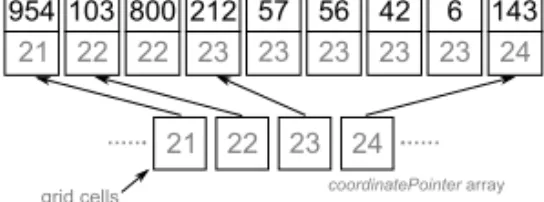
Figure 1. The sorted particleCoordinate array and coordinatePointer array.
integral coordinates are converted to 1D coordinates by Equation 1:
ix+iy× grid width + iz× grid width × grid height. (1) After sorting the particles with respect to their grid coordinates using a radix sort, we determine the number of particles each cell hosts. Figure 1 illustrates the corresponding data structure. The particleCoordinate array stores the sorted particles and thecoordinatePointer array has pointers to the arrayparticleCoordinate for fast access.
The potential neighbors of a particle are determined by following the point-ers from coordinatePointer and by scanning the array particleCoordinate. Constant offsets are employed to access each of the 26 neighboring cells of the particle’s host cell. For example, the (i − 1)th cell is the left neighbor of ith cell and the (i + grid width)th cell is the upper neighbor of the ith cell. Figure 2 illustrates the algorithm where potential neighbors of particle 57 are being searched (within a virtual grid 30 cells wide). The algorithm scans the particles of cell 23 (the host cell of particle 57), cell 24 (the right neighbor cell), and cell 53 (the upper-neighboring cell). To consider each potential neighbor pair exactly once, we scan particles in descending order and terminate when we reach a particle with a smaller ID.
Figure 2. Potential neighbors of particle 57 are being searched.
3.2. GPU-Based Neighbor Search
Particle-based simulations, including SPH, are perfect candidates to be im-plemented on GPUs because of the GPUs ability to process multiple particles in parallel [Pharr and Fernando 05]. The biggest challenge of implementing a particle-based simulation on a GPU is to detect particle proximity efficiently.
This is because of the fact that the fragment shaders that we use as the main processing unit are not capable ofscatter. That is, they cannot write a value to a memory location for a computed address since fragment programs run using precomputed texture addresses only, and these addresses cannot be changed by the fragment program itself. This limitation makes several basic algorith-mic operations (such as counting, sorting, finding maximum and minimum) difficult.
One of the common methods to overcome this limitation is to use a uniform grid to subdivide the simulation space. Kipfer et al. [Kipfer et al. 04] use a uniform grid and sorting mechanism to detect inter-particle collisions on the GPU. Purcell et al. [Purcell et al. 03] also use a sorting-based grid method. They employ a stencil buffer for dealing with multiple photons residing in the same cell. Harada et al. [Harada et al. 07] present a SPH-based fluid simulation system. Their system uses bucket textures to represent a 3D grid structure and make an efficient neighbor search. One limitation of their system is that it can only handle up to four particles within a grid cell.
4. Implementing the Proposed Method on the GPU
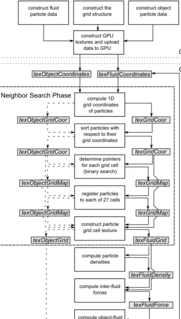
Figure 3 illustrates the work flow of the GPU-based particle simulation that employs the presented technique to compute the particle neighborhood in-formation. Each white rectangle in the figure represents a rendering pass by a fragment program and each gray rectangle represents an RGBA float texture.
4.1. Grid-Map Generation
Algorithm 1 outlines the grid-map generation process. The first two steps of the algorithm compute 1D grid coordinates of particles (Equation (1)), store this information in the grid-coordinate texture (texGridCoor) along with particle IDs, and sort the texture with respect to grid coordinates. The sorting phase employs the bitonic sort [Purcell et al. 03], which makes log2N passes over the texture, whereN is the number of particles.
The next step computes the grid-map texture (texGridMap), which corre-sponds to thecoordinatePointer array in Section 3.1. The fragment program makes a binary search in the sorted grid-coordinate texture for each grid cell to determine the first particle residing in the grid cell and stores this information in the R channel of the grid-map texture.
The final step counts the total number of particles belonging to each grid cell and stores this information in the G channel. Then, a fragment program takes these values in the grid-map texture as input, checks all 26 neighbors
Figure 3. The framework for the GPU-based SPH implementation.
of each grid cell, and determines the total number of particles belonging to each grid cell and its immediate neighbors. This information is stored in the B channel of the grid-map texture. Finally, there is one more pass on the grid-map texture to accumulate the values in the B channel and store this sum in the alpha channel.
Algorithm 1. (The algorithm for grid-map generation.)
for each grid cell i do Step 1:
compute 1D grid coordinates of particles and store in texGridCoor ; Step 2:
sort texGridCoor with respect to 1D grid coordinates ; Step 3:
find first occurrence of i using binary search on texGridCoor (output to channel R); Step 4:
scan texGridMap to determine the number of particles belonging to i (output to channel G);
Step 5:
scan texGridMap to determine number of particles belonging to i and its immediate neighbors (output to channel B);
Step 6:
for j ← 0 to i do
sum the channel G values of j (output to channel A); end
end
Figure 4 depicts a sample grid-map texture. In this figure,
• the values in the R channel point to the first occurrence of the grid cell within the grid-coordinate texturetexGridCoor;
• the values in the G channel are the total number of the particles hosted within the grid cell;
• the B values are the total number of particles hosted in the grid cell itself and its immediate neighbors;
• the alpha-channel values point to the first occurrence of the grid cell with the fluid-grid texture (texFluidGrid), which is generated afterwards.
4.2. Generating Fluid-Grid Texture and Neighbor Lookup
Algorithm 2 outlines the fluid-grid texture generation. Fluid-grid texture (texFluidGrid) is similar to grid-coordinate texture (texGridCoor) in the sense that it contains particle IDs sorted with respect to their 1D grid coordinates. The difference betweentexGridCoor and texFluidGrid is that the latter has an entry for the particle host cell and, additionally, an entry for each of the immediate neighbor cells of the host cell. Each particle appears up to 27 times intexFluidGrid; once for the host cell and 26 times (which could be less if the host cell lies on the grid boundary) for each neighboring cell.
To constructtexFluidGrid, the fragment program has to decide which parti-cle ID is to be stored in the current texture coordinate. Basically, the fragment program determines the grid cell hosting the particle by searching the parti-cles using the alpha channel of the grid-map texturetexGridMap. Then, by following the pointers of the grid cell to the grid-coordinate texture texGrid-Coor, the fragment program finds the appropriate particle ID. For example, assume that the current texture coordinate is 215,425 and the current tex-GridMap is as shown in Figure 4. Binary searching for this coordinate in the alpha channel of the texGridMap reveals that the particle resides in the neighborhood of the grid cell 15,495. Then, to determine the particle ID to store in the current location, we go through the list of hosted particles in the neighborhood of grid cell 15,495.
After generating the textures texGridMap and texFluidGrid, finding pos-sible neighbors of a particle is a simple task. We use the particle’s 1D grid ID to look up the pointer totexFluidGrid. For example, if the 1D grid cell coordinate of particlei is 15,494, then i has 258 potential neighbors starting with 1,807 (see Figure 4).
4.3. Rigid Body–Fluid Particle Neighbor Search
The dashed arrows in Figure 3 show that the rigid-body particles (and solid boundaries) go through the same process to generate particle-grid information. In our case, since the rigid objects do not move during the simulation, the object textures are generated once at the outset. If we choose to move the boundaries or to add moving objects represented by a set of points, then we have to generate particle-grid information for each particle at every time step.
0 1 2 3 4 5 6 7 20 K 40 K 60 K 80 K 100 K 120 K 140 K 160 K 180 K 200 K Fr a me s per S econd Number of Particles NVIDIA 9600 GT NVIDIA 8600 GT NVIDIA 7600 GS CPU
Figure 5. The frame rates of the breaking-dam simulation for different number of particles.
5. Examples
Figure 5 depicts the frame rates of the breaking-dam simulation (Figure 6) on three different NVIDIATM graphics boards and CPU. The test platform
is a PC equipped with an AthlonTM 64 X2 Dual Core processor and 3 GB RAM. The specifications of the tested GPUs are given in Table 1. One of the key observations is that the memory bandwidth is not a crucial factor for the performance since the texture data is uploaded to the GPU memory once, and there are virtually no memory transfers between the system memory and the GPU memory during the simulation. On the other hand, the graphics clock speed and the number of microprocessors have a major impact on the performance because of the parallel nature of the algorithm. Because the CPU version uses Radix Sort that has linear asymptotic complexity, one would expect that the CPU version behaves better for very large datasets. For all of the practical datasets we use for experimentation (up to 200K), the GPU version performs better.
Memory configuration (GDDR3) 256 MB 1024 MB 1024 MB Memory interface width 256-bit 128-bit 256-bit
Memory bandwidth (GB/sec) 42.2 22.4 57.6
Table 1. The specifications of the GPUs used in the dam-breaking scene.
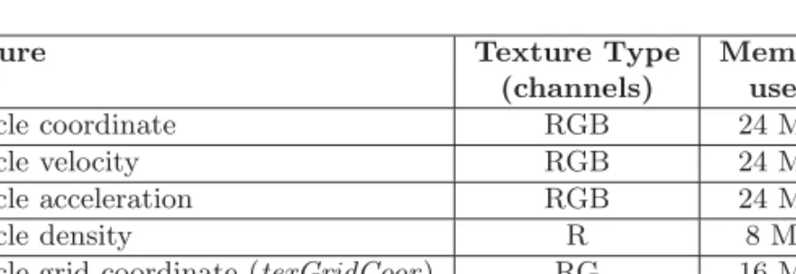
Texture Texture Type Memory
(channels) used
Particle coordinate RGB 24 MB
Particle velocity RGB 24 MB
Particle acceleration RGB 24 MB
Particle density R 8 MB
Particle-grid coordinate (texGridCoor ) RG 16 MB
Grid-map texture (texGridMap) RGBA 32 MB
Fluid-grid texture (texFluidGrid ) RG 432 MB
Table 2. The memory requirements of a SPH simulation based on the proposed neighbor-search algorithm. The texture dimension is 2048× 1024.
The memory requirements of the dam-breaking simulation are shown in Table 2. The size of textures allocated to store particle information is 2048× 1024 (storage space for more than two million particles). The total memory requirement of the simulation is 560 MB.
Figure 7 shows still frames from a simulation where fluid particles flow down onto a fountain model. The fluid body consists of 64K particles at the end of the simulation, and the fountain object consists of about 64K particles. The frame rate we obtain for the simulation is approximately 2 fps on an NVIDIA
Figure 8. Fluid particles flow into a cloth mesh.
8600 GT. If we use the neighbor-search algorithm for the CPU, we obtain a frame rate of approximately 0.5 fps.
In Figure 8, fluid particles flow into a cloth mesh that is simulated by a mass-spring network. The cloth mesh is composed of 20K particles, and collisions between the cloth and the fluid particles are detected by the proposed method. The frame rate is 5 fps on an NVIDIA 8600 GT.
6. Conclusion
This paper presents a neighbor-search algorithm to be used in particle-based simulations. The algorithm sorts particles with respect to their grid coor-dinates and registers them to their neighboring grid cells. It then looks for potential particle proximities by using this grid-particle map. The main fo-cus of the paper is to propose a method to overcome the current inability of fragment shaders to do scatter operations.
The primary strength of the proposed method is that it does not, unlike the existing techniques, make an assumption about the particle density, the radius of the neighbor search, the number of grid cells, and the grid-cell size. This is especially important when simulating compressible fluids and dense natural phenomena, e.g., sand, smoke, and soil. The algorithm yields optimum performance if the radius of the neighbor search is one cell.
The main shortcoming of the method is that it is slower than the simi-lar sorting-based grid methods for fixed grid particle density, e.g., [Harada et al. 07]. This is because of the expensive grid-map generation phase in our method. As a future work, the method can be implemented by using Compute Unified Device Architecture (CUDA), which has scatter capabilities.
References
[Cleary et al. 07] P. W. Cleary, S. H. Pyo, M. Prakash, and B. K. Koo. “Bubbling and Frothing Liquids.” ACM Transactions on Graphics 26:3 (2007), Article No. 97, 6 pages.
[Harada et al. 07] T. Harada, S. Koshizuka, and Y. Kawaguchi. “Smoothed Parti-cle Hydrodynamics on GPUs.” In Proc. of Computer Graphics International, pp. 63–70. Geneva: Computer Graphics Society, 2007.
[Kipfer and Westermann 06] P. Kipfer and R. Westermann. “Realistic and Interac-tive Simulation of Rivers.” In GI ’06: Proceedings of Graphics Interface ’06, pp. 41–48. Toronto: Canadian Information Processing Society, 2006.
[Kipfer et al. 04] P. Kipfer, M. Segal, and R. Westermann. “UberFlow: A GPU-Based Particle Engine.” In Proc. of the ACM SIGGRAPH/EUROGRAPHICS
Conference on Graphics Hardware, pp. 115–122. Aire-la-Ville, Switzerland:
Eu-rographics Association, 2004.
[Melax 00] S. Melax. “Dynamic Plane Shifting BSP Traversal.” In Proc. of Graphics
Interface ’00, pp. 213–220. Toronto: Canadian Information Processing Society,
2000.
[Miller and Pearce 89] G. S. P. Miller and A. Pearce. “Globular Dynamics: A Con-nected Particle System for Animating Viscous Fluids.” Computers and
Graph-ics 13:3 (1989), 305–309.
[Monaghan 92] J. J. Monaghan. “Smoothed Particle Hydrodynamics.” Annual Review of Astronomy and Astrophysics 30 (1992), 543–574.
[M¨uller et al. 03] M. M¨uller, D. Charypar, and M. Gross. “Particle-Based Fluid Simulation for Interactive Applications.” In Proc. of the ACM
SIG-GRAPH/Eurographics Symposium on Computer Animation, pp. 154–159.
Aire-la-Ville, Switzerland: Eurographics Association, 2003.
[M¨uller et al. 04] M. M¨uller, S. Schirm, M. Teschner, B. Heidelberger, and M. Gross. “Interaction of Fluids with Deformable Solids.” Journal Computer Animation
and Virtual Worlds 15:3–4 (2004), 159–171.
[Pharr and Fernando 05] M. Pharr and R. Fernando. GPU Gems 2: Programming
Techniques for High-Performance Graphics and General-Purpose Computation.
Reading, MA: Addison-Wesley Professional, 2005.
[Purcell et al. 03] T. J. Purcell, C. Donner, M. Cammarano, H. W. Jensen, and P. Hanrahan. “Photon Mapping on Programmable Graphics Hardware.” In
Proc. of the ACM SIGGRAPH/EUROGRAPHICS Conference on Graphics Hardware, pp. 41–50. Aire-la-Ville, Switzerland: Eurographics Association,
2003.
[Reeves 83] W. T. Reeves. “Particle Systems - A Technique for Modeling a Class of Fuzzy Objects.” ACM Transactions on Graphics 2:2 (1983), 91–108.
[Terzopoulos et al. 91] D. Terzopoulos, J. Platt, and K. Fleischer. “Heating and Melting Deformable Models.” The Journal of Visualization and Computer
An-imation 2:2 (1991), 68–73.
[Teschner et al. 03] M. Teschner, B. Heidelberger, M. M¨uller, D. Pomerantes, and M. H. Gross. “Optimized Spatial Hashing for Collision Detection of Deformable Objects.” In Proc. of Vision, Modeling, Visualization (VMV’03), pp. 47–54. Aka GmbH: Heidelberg, Germany, 2003.
[Teschner et al. 04] M. Teschner, S. Kimmerle, G. Zachmann, B. Heidelberger, L. Raghupathi, A. Fuhrmann, M.-P. Cani, F. Faure, N. Magnetat-Thalmann, and W. Strasser. “Collision Detection for Deformable Objects.” In Eurographics
State-of-the-Art Report (EG-STAR), pp. 119–139. Aire-la-Ville, Switzerland:
Eurographics Association, 2004.
[Tonnesen 91] D. Tonnesen. “Modeling Liquids and Solids Using Thermal Parti-cles.” In Proc. of Graphics Interface ’91, pp. 255–262. Toronto: Canadian Information Processing Society, 1991.
Web Information:
Additional material can be found online at http://jgt.akpeters.com/papers/ BayraktarEtAl09/
Serkan Bayraktar, Department of Computer Engineering, Bilkent University, 06800, Bilkent, Ankara, Turkey ([email protected])
Uˇgur G¨ud¨ukbay, Department of Computer Engineering, Bilkent University, 06800, Bilkent, Ankara, Turkey ([email protected])
B¨ulent ¨Ozg¨u¸c, Department of Computer Engineering, Bilkent University, 06800, Bilkent, Ankara, Turkey ([email protected])