Money demand, the Cagan model, testing rational expectations vs adaptive expectations: the case of Turkey

(1)

QEMAHD-, T H l CAMAM MOOEl^

mm

IE OF 1

B t ¡ L M m

M u s - t y

A / o

f O o 6 . s

f 3 S s

T H s IHSTITUTE

ECOHOMiCS AND SOCIAL SCIEMCES

m FA ETfA i EULFILLMEFiT OF THE

a E M i i

FOat THE DBQREt OF M

a

S T

c

I

l

OF

JL _{Say#'\jfiVS^i№}

(2)

MONEY DEMAND, THE CAGAN MODEL, TESTING RATIONAL EXPECTATIONS vs

ADAPTIVE EXPECTATIONS: THE CASE OF TURKEY

A THESIS PRESENTED BY İLKER MUSLU TO

THE INSTITUTE OF

ECONOMICS AND SOCIAL SCIENCES IN PARTIAL FULFILLMENT OF THE

REQUIREMENTS f o r t h e d e g r e e o f m a s t e r o f ECONOMICS BILKENT UNIVERSITY July, 1995 -il __ M us.li farofindcn bcği}lamtu§fır.

(3)

Н й -i - ‘5

-1 S 3 5

(4)

I certify that I have read this thesis and in my opinion it is fully adequate, in scope and in quality, as a thesis for the degree o f Master o f Economics.

e

Assist.Prof Dr. Kıvılcım METİN

I certify that I have read this thesis and in my opinion it is fully adequate, in scope and in quality, as a thesis for the degree o f Master o f Economics.

"/

q

J

i u j x uv"—.

Assist.Prof Dr. Fatma TAŞKIN

1 certify that I have read this thesis and in my opinion it is fiilly adequate, in scope and in quality, as a thesis for the degree o f Master o f Economics.

7

Assist.Prof Dr. Nedim ALEMDAR

(5)

ABSTRACT

MONEY DEMAND, THE CAGAN MODEL, TESTING RATIONAL EXPECTATIONS vs

ADAPTIVE EXPECTATIONS: THE CASE OF TURKEY

İL K E R M U SLU M aster o f Econom ics

Supervisor: A ssist.Prof.D r. K ıvılcım M ETİN July, 1995

This thesis considers the demand for money under conditions o f high inflation in Turkey during the period 1986; 1-1995:3. We test whether the monetary and

inflationary experiences o f Turkey can be adequately characterized by the Cagan (1956) model, using an econometric procedure which is reliant only on the assumption that forecasting errors are stationary. We also examine the hypothesis that monetary policy was conducted in such a way as to maximize the inflation tax revenue. Finally w e test the Cagan model with the additional assumption o f rational expectations for Turkey for the considered period.

Keywords: Adaptive Expectations, Cointegration, Hyperinflation, Inflation Tax, Money Demand, Rational Expectations, Unit Root.

(6)

o z

PA RA t a l e b i, g a g a n M O D E Lİ, R A SY O N E L B E K L E N T İL E R İN U Y A R L A N A B İL İR B E K L E N T İL E R E K A R ŞI T E S T E D İL M E S İ: T Ü R K İY E U Y G U LA M A SI İL K E R M U SLU

Y üksek L isans Tezi, İk tisa t Bölüm ü Tez Y öneticisi: Y rd.D oç.D r. Kıvılcım M ETİN

T em m uz, 1995

Bu tez Türkiye’de 1986:1-1995:3 dönemindeki yüksek enflasyon koşulları altındaki para talebini incelemektedir. Tezde, Türkiye’de bu dönemde yaşanan parar>al ve enflasyonist tecrübelerin C agan’m (1956) modeli ile tam olarak nitelenmesinin mümkün olup olmadığı ekonometrik bir yöntem kullanılarak test edilmiştir. Ayrıca söz konusu dönemde otoritelerce yürütülen para politikasının enilasyon vergisini

maksimize edecek şekilde olduğu hipotezi incelenmiştir. Son olarak da C agan’ın modeli rasyonel beklentiler varsayılarak Türkiye için yukarıdaki dönem gözönünt alınarak test edilmiştir. ‘

Anahtar Kelimeler: Birim Kök, Hiperenflasyon, Enflasyon Vergisi, Kointegrasyon, Para Talebi, Rasyonel Beklentiler, Uyarlanabilir Beklentiler.

(7)

Acknowledgments:

I would like to express my gratitude to Assist.Prof.Dr. Kıvılcım Metin for her close supervision and suggestions during the preparation o f this thesis. I would also like to thank Assist.ProfDr. Fatma Taşkın and Assist.Prof Dr. Nedim Alemdar for reading and evaluating this thesis.

(8)

TABLE OF CONTENTS

I - INTRODUCTION

Page

2

II - AN OVERVIEW OF TURKISH EC O N O M Y

III - CAGAN’S HYPERINFLATION M OD EL

IV - METHODOLOGY 4.1. Stationarity 4.2. Unit Roots

4.2.1. Introduction 4.2.2. Unit Root Tests 4.3. Cointegration Analysis 13 13 16 16 16 19 V - EMPIRICAL RESULTS 5.1. The Model

5.2. The Data Set

5.3. Unit Roots and Testing for the O rder o f Integration

5.4. Testing for Cointegration (Testing for Adaptive Expectations) 5.5. Testing the Rational Expectations Hypothesis

23 23 24 25 30 35 VI - CONCLUSION 37 REFERENCES 39 APPENDICES 42

(9)

I - INTRODUCTION

Cagan (1956) formulated a specific version o f the demand for money function and a specific hypothesis about the formation o f inflationary expectations. Cagan’s paper posed and dealt with questions about the role o f money in generating inflation. His paper produced results that have had wide range o f applications in the context o f monetary approach to inflation. Cagan confined his study to hyperinflations where, he argued, fluctuations in the price level and the inflation rate swamped those in real income or the rate o f return on capital goods. Hence, he formulated a demand for real money balances function in which the only argum ent was the expected inflation rate. Further, Cagan assumed adaptive expectations about inflation.

Cagan (1956) deals with the relation between changes in the quantity o f money and price level during hyperinflations. Cagan defines hyperinflations as beginning in the month the rise in prices exceeds 50 percent and as ending in the month before the monthly rise in prices drops below that am ount and stays below for at least a year.

This thesis considers the demand for money under conditions o f high inflation in Turkey during the period 1986:1-1995:3. We test whether the monetary and

inflationary experiences of Turkey can be adequately characterized by the Cagan (1956) model, using an econometric procedure which is reliant only on the assumption that forecasting errors are stationary. Engle (1982) demonstrates that forecasting errors would be stationary under adaptive expectations.

Turkey has not experienced such a hyperinflation in the Cagan’s sense, but high rates o f inflation have been seen in Turkey during the period 1986-1995. Taylor and Phylaktis (1991) examined the demand for m oney under conditions o f high inflation in some Latin American countries, during the 1970s and 1980s, using Cagan’s

hyperinflation model and these countries also have not experienced hyperinflation in the Cagan’s sense. If the Cagan model is applicable to Turkey, then it can be a

powerful tool o f analysis in understanding the features o f the monetary' experiences o f Turkey.

(10)

It is well known that generating inflation through printing money can be viewed as a means o f raising revenue for the authorities-an inflation tax. Cagan (1956) shows that, in the context o f the hyperinflation model, the revenue from the inflation tax, which results from money creation by the authorities, is maximized by a certain percentage rate o f increase in prices and money. In the thesis, we test the hypothesis that the authorities expanded the money supply in such a way as to maximize the inflation tax revenue in Turkey for the considered period.

During the period 1986-1995, excluding 1994, Turkey experienced a stable annual inflation rate o f sixty percent to seventy percent. This can be taken as a clue for rational expectations. This encouraged us to derive a test o f the Cagan (1956) model with the additional assumption o f rational expectations for Turkey for the considered period. Under the additional assumption o f rational expectations, this implication o f the hyperinflation model is a particular case o f a general result for present value models discussed by Campbell and Shiller (1987).

In this thesis, section II gives a brief overview o f the Turkish economy. Cagan’s hyperinflation model is explained in section III and the methodology is described in section IV. In section V estimation results are presented and we concluded the results o f the thesis in section VI.

(11)

II - AN OVERVIEW OF TURKISH ECONOMY

After a period of economic and politic difficulties, some mixed stabilization and liberalization policies were announced by the Turkish government in January 1980. The announced policies aimed a new adjustment path with a new export lead

development strategy. Main topics o f the policies were the convertibility o f the Turkish lira, flexible exchange rate policy and export promotions. As a component o f the programme, there was a major devaluation o f the Turkish lira in January 1980. The

1980 programme also included positive real interest rate policy. As a result o f these policies in 1981-1983 period the inflation rate did not exceed 36%.

In the period 1984-1987, the average inflation rate was around 40%. In April 1986, the Central Bank set up an Interbank m arket for one and two week maturities and introduced overnight transaction in M ay 1986. In 1986, the Central Bank introduced for the first time the policy approach o f targeting a monetary aggregate. Money in wider sense (M2) was selected to be kept on a growth path during the year. In 1986, M2 grew 38.6%, which was close to the target level. In 1986, M l had a growth o f 62.5% and reserve money had a grow th o f 32.8% and the consumer price inflation achieved 34.6%. For 1987 the m onetary authorities targeted growth o fM 2 at 30 percent which was considered consistent with an expansion o f 5 percent and an inflation rate o f 25 percent. The Central B ank had planned 28 percent growth o f the reserve money which was the main instrum ent to control M2. But reserve money growth was nearly 50 percent in 1987 and consum er price inflation was 38.9 percent. In 1987, M l growth was 58.3% and M 2 grow th was 37.6%.

Growing public sector deficits has been a traditional problem o f Turkish economy for many years. Largeness and incapability o f the public economy has been the main causes o f the growing public sector deficits. Deficits o f the State Economic Enterprises (SEEs) and wasting the public w orker’s fee resources can be shown as examples to the incapability o f the public economy. High debt interest payments, insufficient adjustment o f prices o f State Economic Enterprises to increased costs and a large increase in the public sector wage bill were the main factors behind the growing public sector deficits.

(12)

In view o f accelerating inflation and instability in financial markets, monetary policy was severely tightened in 1988. D eposit interest rates were raised to encourage financial savings and reduce the share o f currency and sight deposits in M2. But, in spite o f this tightening policy, targets w ere exceeded by substantial amount in 1988. M l, M2 and reserve money grovvih w ere 39.7% , 77.5% and 67.5%, respectively. Consumer price inflation reached 75.4% in 1988.

In 1989 as a result o f decree num ber 32 that is put into use, Turkish lira has become completely convertible across other foreign currencies and financial capital has become completely free to enter and leave the country. At this point to gain the macro financial balance in the country, exchange rate and domestic interest rate became integrated and real return from interest rate was higher than the real return from foreign currency. As a result, dolarization was prevented and domestic currency has been used widely and foreign capital entered the country.

For 1989, the Central Bank has abstained from announcing monetary targets. In 1989, reserve money growth accelerated due to increase in net foreign assets and due to the government’s decision to grant large salary increases and to raise agricultural support prices. Reserve money grow th reached 75% and M l and M2 growth were 97.1% and 82%, respectively. In 1989, consum er price inflation was at the level o f 69.6%. In the context o f the program m e o f economic liberalization, the Turkish authorities have been aiming at placing g reater reliance on monetary policy for economic stabilization purposes. H ow ever, as the Central bank is not completely autonomous and economic policy decisions are taken at the government level, it has been difficult to follow a! clear anti-inflationary monetary policy.

Starting from 1990’ interest rate-exchange rate balance and foreign capital inflow have directly depended on each other. In 1990 return from interest was 2.5% above the return from foreign currency and this caused 3000 million dollars o f foreign capital inflow. In 1991 the return from interest over return from foreign currency fell to -3.3% and this caused 3020 million dollars o f capital to leave the country. From this time after, return from interest have been always above the return from foreign currency and in 1992 and 1993 there have been seen net foreign capital inflow. In 1993 Total

(13)

Capital Movements item has reached 9279 million dollars and this value is 5.6% o f G N Pin 1993.

In this way it was aimed to cover public sector’s deficits by savings from outside. But this also brought about increase in volume o f imports. Public sector was continuing high interest rate policy by domestic credit and high interest rate was bringing about financial capital entrance into the economy. But this procedure has directly affected the goods market and there have been seen many cycling in the real production sectors. This was because that under the above procedure what was determining the exchange rate was not the international good and service trade, but it was the capital movements that depended on speculative demand determ ining the exchange rate. As a result exports have fallen and imports have risen. In 1989 the ratio o f exports to imports was 0.736 but in 1993 the ratio has fallen to 0.516. Inflation has reached an average o f 68.2% in the period 1988-1992. M onetary policy aimed at maintaining orderly conditions in financial markets. The Central bank, however, was again obliged to finance the PSBR, and hence fiscal imbalance induced rapid growth in the monetary aggregates. In the period 1988-1992, M l, M2 and reserve money growth reached an average o f 62%, 67% and 58%, respectively.

Strong output grovidh in 1992 and 1993, led by domestic demand, brought about a widening current account deficit and rising foreign indebtedness. Inflationary

pressures intensified, partly in response to the further increase in public sector deficits to very high levels. In 1993 real GNP grow th averaged 6.75%, the trade deficit rose to

12% o f GNP and public sector borrowing requirement (PSBR) rose to 16% o f GNP. Ajinual consumer price inflation averaged 66% in 1993, compared with 70% in 1992. At the end o f 1993, international creditworthiness was downrated and the Turkish lira drastically depreciated. M l, M2 and reserve money growth were 53%, 43% and 60%, respectively in 1993.

Starting in 1994, Turkish economy have undergone the most important crisis o f the last 15 years. The crisis has started in the first months o f 1994 in finance market and it has spread to the real part o f the econom y in a little time. The main causes o f

(14)

the crisis has been shown as the grow ing public sector deficits and the incorrect steps towards liberalization.

On 5 April 1994, the governm ent announced a new programme. Prices o f goods and services produced by SEEs w ere immediately raised by 110 percent. The new programme also envisages accelerated closure and privatization o f SEEs, a decrease in public sector real wages and other unspecified public expenditure cuts. After the announcement o f the package the Turkish lira depreciated further by about 35%, to some 60% below the level at the beginning o f the year. Also the economic expansion stopped and there was a short term increase in inflation. Higher inflation, public sector wage restraint and labour shedding eroded real household incomes and depressed private consumption. Consumer price inflation was 126%, and wholesale price inflation was 150% in 1994. Public sector borrowing requirement fell to 8% o f GNP. In 1994, M l, M2 and reserve money grow th reached 85%, 132% and 85%,

respectively. In April 1995, the annual consum er price inflation achieved 94%. And in April 1995, the three months M l, M2 and reserve money growth ratios achieved

(15)

Ill - CAGAN'S HYPERINFLATION MODEL

Cagan (1956) deals with the relation between changes in the quantity o f money and price level during hyperinflations. An outstanding characteristic o f such periods is the decline in the real value o f the quantity o f money-real cash balances

(M/P).

Cagan defines hyperinflations as beginning in the month the rise in prices exceeds 50 percent and as ending in the month before the m onthly rise in prices drops below that amount and stays below for at least a year. The theory developed by Cagan (1956) involves an extension o f the Cambridge cash-balances equation. That equation asserts that real

cash balances remain proportional to real income

(V)

under given conditions

(M/P

=

kY; k is a constant).

Cagan (1956) discusses that individuals’ desired real cash balances depend on numerous variables. The main variables that affect an individual’s desired real cash balances are his wealth in real terms, his current real income and the expected returns from each form in which wealth can be held, including money. Desired real cash balances change in the same direction as real wealth and current real income and in the direction opposite to changes in the return on assets other than money. A specification o f the amount o f real cash balances that individuals want to hold for all values o f the variables listed above defines a demand function for real cash balances. Other variables usually have only minor effects on desired real cash balances and can be omitted from the demand function. This demand function and the other demand and supply

functions that characterize the economic system simultaneously determine the equilibrium amount o f real cash balances.

In one theory o f this determ ination-the quantity theory o f money-the absolute level o f prices is independently determined as the ratio o f the quantity o f money supplied to a given level o f desired real cash balances. Individuals can not change the nominal amount o f money in circulation, but, according to the quantity theory o f money, they can influence the real value o f their cash balances by attempting to reduce or increase their balances. In this attempt they bid the prices o f goods and services up or down, respectively, and thereby alter the real value o f cash balances.

(16)

Cagan (1956) discusses that during hyperinflation the amount o f real cash

balances changes drastically. At first sight these changes may appear to reflect changes in individuals’ preferences for real cash balances, but these changes in real cash

balances may reflect instead changes in the variables that affect the desired level o f balances. Cagan observ’ed that tw o o f the main variables affecting individuals’ desired level, wealth in real terms and real incom e, w ere relatively stable during hyperinflation, at least compared with the large fluctuations in real cash balances. Thus he decided to look for large changes in the only rem aining variable, which is the expected rcaim s on various forms o f holding wealth, to explain large fluctuations in the desired level o f real cash balances. Changes in the return on an asset affect real cash balances only if there is a change in the difference between the expected return on the asset and that on money. If this difference rises, individuals will substitute the asset for part o f their cash balances. So Cagan turned to a m ore detailed consideration o f the difference in return on money and on various alternatives to holding money-the cost o f holding cash balances.

Cagan also observed that the only cost o f holding cash balances that fluctuate widely enough to account for the drastic changes in real cash balances during

hyperinflation is the rate of depreciation in the value o f money or, equivalently, the rate o f changes in prices. This observation suggested the hypothesis that changes in real cash balances in hyperinflation result from variations in the expected rate o f change in prices. Cagan assumed that desired real cash balances are equal to actual real cash balances at all times. This means that any discrepancy that may exist between the two is erased almost immediately by m ovem ents in the price level. He also assumed that the expected rate o f change in prices is revised per period o f time in proportion to the difference between the actual rate o f change in prices and the rate o f change that was expected.

Cagan’s model is composed o f tw o equations, an equation giving the demand for money and an equation describing the form ation o f expectations. The monetary equilibrium is given by

(17)

where

c

and

a

are constant terms and k is the expected rate o f inflation. The higher expected inflation, the lower will be the demand for real money balances. Two important assumptions are implicit in this formulation. The first is that output is given and thus is part o f the constant term

c.

The second is that the real interest rate is constant and thus also included in the constant term

c.

The main rationale for this functional form is convenience, though it appears consistent with the data from hyperinflations. In an equilibrium the real money stock must be equal to money demand, and ( 3.1 ) can be interpreted as an equilibrium equation. An implication o f the above relation is that variations in the expected rate o f changes in prices have the same effect on real cash balances in percentage terms regardless o f the absolute amount o f the balances. This follows from the fact that equation (3 .1 ) is a linear relation between the expected rate o f change in prices and the logarithm o f real cash balances.

From equation ( 3.1 ), the elasticity o f demand for real cash balances with respect to the expected change in prices can be written as

d(M/P) drc*

71

M/P -

ajK

where

art

is a pure number. The elasticity is proportional to the expected rate o f

change in prices. It is positive when expected inflation rate is negative, and negative when expected inflation rate is positive.

The second equation Cagan used describes the formation o f expectations. Cagan assumed adaptive expectations about inflation. Under adaptive expectations,

expectations o f inflation are adjusted according to

dTcVdt = b(7t - 7t’ ), ( 3 . 2 )

where ;ris the actual inflation rale. I f current inflation exceeds expected inflation,

expected inflation increases. The coefficient

b

reflects the speed at which individuals

(18)

revise their expectations. Note that the expected inflation depends only on past inflation. Equation ( 3.2 ) can be integrated to yield

>r*t = bJU 71, exp[b(s - t)] ds.

Given the dynamics o f money growth, equations ( 3 .1 ) and ( 3.2 ) determine the dynamics o f inflation.

Cagan (1956) studied if inflation will converge to cr or it will take o ff on its own toward hyperinflation when money grow th is constant at rate cr. To answer this question differentiate equation ( 3 . 1 ) after taking logarithms. This gives

a - K = -a(dn’/dt).

( 3 . 3 )

Eliminating

dn/dt

between ( 3.2 ) and ( 3.3 ) gives the relation

a - n =

-ab(7t - 7t*). ( 3 .4 )

Cagan showed that a self-generating inflation is impossible if the product o f the

parameters

a

and

b

is less than unity. Thus econometric estimates o f these two

parameters provide vital evidence on the stability o f the inflationary process. Cagan estimated his model using data on seven hyperinflations and was not able to reject the hypothesis that the stability conditions w ere satisfied. He found out that, in these seven hyperinflations, the sensitivity o f the dem and for money to the expected rate o f

inflation and the sensitivity o f the expected inflation rate to the actual rate are both small enough to rule out a self-generating inflation.

If

ab >

1, then the equilibrium is unstable. In the unstable case, depending on the initial conditions, the economy can have either accelerating inflation or accelerating deflation. Thus whether there can be hyperinflation under constant money growth

depends on the parameters

a

and

b,

which reflect respectively the elasticity o f money

demand and the speed of revision o f expectations. Why is the equilibrium unstable if

(19)

ah>

1? If ^ is large, higher inflation leads money holders to quickly revise upward their expectations o f inflation and thus to attempt to reduce their money holdings; given money growth, this leads to fLirther inflation, further revisions, and accelerating inflation. If

a

is large, an increase in inflation that leads to an upward revision o f expected inflation has a strong negative effect on money demand, leading again to accelerating inflation. Accordingly, if individuals have adaptive expectations, it is possible for hyperinflation to result not from accelerating money growth but rather from a self-generating unstable process.

Cagan (1956) also studied the maximum amount o f revenue, that is available, from the inflation tax, if the equilibrium is stable. The inflation tax is the tax imposed on money holders as a result o f inflation, i.e., it is the loss in the value o f money holders’ real balances. Inflation tax is equal to

dP/dt M M

1 = --- — =Tc —

P P P ( 3 . 5 )

Using equation ( 3 . 1 ) and the fact that in steady state (without growth) k

=

cr gives

I = Ttcexp(-aa).

Accordingly, steady state inflation tax is maximized when cr= l / o : . So the percentage increase in prices and money, which maximizes the revenue from the inflation tax, is just equal to (100/a)% .

(20)

IV - METHODOLOGY

4 .1 . Stationarity

A stochastic process is said to be

stationary,

if the joint and conditional

probability distributions o f the process are unchanged if displaced in time. In practice, it is more usual to deal with

weak sense

stationarity, restricting attention to the means, variances and covariances o f the process ( Spanos 1986). Consider a simple time series model as follows;

yt = ayt-i + 6t,

where £,is the uncorrelated disturbance term with zero mean and constant variance. In

such a model, if

a

is less than 1 in absolute value, the observations fluctuate around

zero. Such series in econometrics is said to be stationary. On the other hand, if the absolute value o f

a

is greater than 1, the model is explosive.

Then, a stochastic process is said to be

stationary

if:

and:

E(yt) = constant = p; Var(yt) = constant =

Cov(yiytH-j) = aj.

Thus the means and the variances o f the process are constant over time, while the value o f the covariance between two periods depends only on the gap between the periods, and not the actual time at which this covariance is considered. If one or more o f the conditions above are not fulfilled, the process is nonstationary.

Equivalently a time series is said to be

stationary

if

yt = E(yt) + St,

(21)

and

E(s,) = 0, E(8^) =

E (S (8s) = 0 t s.

Therefore a stationary series is said to tend to fluctuate around its mean with broadly constant amplitude. Whereas a nonstationary time series will have a time varying mean and variance so that cannot be referred without reference o f some particular time period.

An important type o f a nonstationary stochastic process is the process which is

called

random walk.

The main assumption is that, every current observation consist o f

its own previous value plus a random disturbance term and disturbance terms are identically distributed independent random variables:

yt = y,-i + 8,, E(st) = |i, E(8^) =

E (8 t8 s) = 0 t Vi: S.

Another example o f a nonstationary stochastic process is:

yt = a + y,-i + 8,, avtO,

where £,is defined as before as a series o f identically distributed independent random

variables and

a

is constant. This stochastic process is called a

random walk with drift.

If the errors £>are identically distributed independent random variables with zero means, then the stochastic process

St

is called a

white noise process.

In economics, the form o f nonstationarity in a time series may well be evident from an examination o f the series. If the form o f nonstationarity is a propensity o f the series to move in one

direction, we will call this tendency a

trend.

(22)

A series may drift slowly upwards or downwards purely as a result o f the effects o f stochastic or random shocks. This is true for the random walk process. The variance o f this process increases over time and also the correlation between neighbouring values increases over time. These results imply that there may be long periods in which the process takes values well away from its mean value. Such series is called a time

series with a

stochastic trend.

Another example of a developing tendency in a nonstationary stochastic process is where the mean of the process is itself a specific function o f time. If such a function is linear then the process can be described as;

where:

or:

yt = Pt + St,

Pt = a + pt,

yt= a + pt + St.

In this case it is said the process has a

deterministic trend.

A mixed stochastic-

deterministic trend process is also possible. That is, the process can be described as:

y^= a + pt + yn + 8t.

In these expressions, it has been assumed that the expected values o f ¿/are zero

and that the stochastic process

s,

is white noise, but these conditions may be relaxed to

allow for autocorrelation in the series o f

St.

Stationarity is an important concept in time series modeling. However, many time series, in economics, are not stationary. But nevertheless, by taking first or second differences, a nonstationaiy series can be transformed to a stationary series.

Sometimes it is necessary to difference a series more than once in order to achieve stationarity. A nonstationary series which can be transformed to a stationary series by

(23)

differencing J times is said to be

integrated o f order d

( Engle and Granger 1987 ). A series integrated of order

d

is denoted as>', ~ 1(d).

4 .2 . Unit Roots

4 .2 .1 . Introduction

As we indicated above, in the time series, a statistical time series may be difference stationary. Consider a simple difference stationary series:

yt = yt-i + St,

where ffis an independent, normal, zero mean stationary process. In such a model the effect o f a shock is permanent. Any jum p in

s,

will cause increase in all>'/s. On the other hand if the shock fades away then w e assume the model to be:

y t= a y t- i+ 8 t a < l .

Therefore, whether there is a unit root or not ( a = 1 or a < 1 ), becomes a very important issue for economists.

4 .2 .2 . Unit Root Tests

Suppose we wish to test the hypothesis that a variable y, is integrated o f order one, that is that>^, is generated by:

yt = yi-i +

Si,

where

St

represents a series o f identically distributed stationaiy variables with zero

means.

(24)

A straightforward procedure would seem to test for or = 1 in the model:

Yi = ayi-i + 8t. ( 4 .1 )

An appropriate and simple method o f testing the order o f integration of^', has been

proposed by Dickey and Fuller (1979) which is called the

DF test.

The DF test is a test

o f the hypothesis that in ( 4.1 ) a = 1, the so-called

tmit root test.

This test proposes a simple method o f testing for a = 1 or a < 1. Instead o f equation (4.1 ) we can write

where

Ayt= 5yn + St,

a = 1 + 5.

( 4 . 2 )

Then the test is simply testing

5 = 0 or 5 <0.

I f ¿'is significantly negative then

cc

< 1 and the series are time stationary. W hereas, if ¿ = 0 then

a =

1 and the series has a unit root. So the Dickey-Fuller test consists o f testing the negativity o f ¿ in the ordinary least squares regression o f (4 .2 ). Rejection o f the null hypothesis ¿ = 0 in favor o f the alternative ¿ < 0 implies that a < 1 and thaty', is integrated o f order zero.

Since in ( 4.2 ) we want to evaluate a hypothesis which concerns only a single parameter, the natural choice would seem to be that of a Student t-ratio. But, for equation ( 4 .2 ) , this ratio or statistic does not have the familiar Student t-distribution. Because o f the unit root, the t-ratio does not have a limiting normal distribution. Therefore, the simulated DF critical values table are used for comparison. Critical values for the DF test statistics are tabulated in Fuller (1976), table 8.5.2.

If the null hypothesis can not be rejected, the variable y, might be integrated o f order higher than zero, or might not be integrated at all. Consequently the next step would be to test the order of integration is one. Hence, we repeat the test for;

AAyt = 5Ayi.i + 8t,

(25)

and again our interest is in testing the negati\Tty o f (5. If the null hypothesis is rejected and the alternative S < 0can be accepted, the series _y,~ 1(1). If the null hypothesis can not be rejected, we may test whether >v ~ 1(2). We can continue the process until we establish an order o f integration for>',. B ut this process creates a danger o f

overdifferencing, which results in a very high positive value o f DF test accompanied by a very high coefficient o f determination for the fitted regression. Such cases indicate that either the series is integrated o f som e order but the test fails to discover this or, the series is not an integrated time series and differencing cannot transfer it into a

stationary series.

The DF test can also be used for testing the order of integration for a variable generated as a stochastic process with drift, that is by tests on the equation:

Ayt= a + 5y,.i + et,

where a is a constant representing drift. A modification of the DF equation which accounts for both drift and a linear deterministic trend is the following;

Ayt = a + Pt + 5yt-i + 8t.

A weakness o f the DF test is that it does not take account o f possible

autocorrelation in the error process. I f

e,

is autocorrelated, then the ordinary least squares estimates o f equation (4 .2 ) are not efficient. A simple solution, advocated by Dickey and Fuller (1981), is to use lagged left-hand side variables as additional

explanatory variables to iapproximate the autocorrelation. This test is called

Augmented

Dickey-Fuller (ADF) test.

The ADF tests involve estimating the equation:

Ayt= 5 y n + ZViSiAyt-i + 8t,

The value o f

k

must be small enough to save the degrees o f freedom, but large

enough to capture the autocorrelation in the error process. The testing procedure is the same as DF, with an examination o f the Student t-ratio for

5

and the critical values are

(26)

the same as for the DF test. A modification o f the ADF equation which accounts for drift is the following:

Ayt = a + 5yt-i + Z'"i=i5iAyt.i + St.

A modification o f the ADF equation which accounts for both drift and a linear deterministic trend is the following;

Ayt = a + pt + 5yi-i + Z^=ı6iAyt.i + 8t.

4 .3 . Cointegration Analysis

Time series

x, andy,

are said to be

cointegrated

of order d, b where d > b > 0, written as: Xf,

yt

~ CI(d, b), if:

i. both series are integrated o f order

d,

ii. there exists a linear combination o f these variables, say aiXt + aayt, which is integrated o f order c/ -

h.

The vector [ a i, a^] is called a

cointegrating vector.

A generalization o f the above definition is the following. If x, denotes an n x 1 vector o f series and;

i. each o f them is 1(d),

ii. there exists an n x 1 vector

p

such th at x'». P = ~ I(d - b), then:

x\.

P ~ CI(d, b).

The vector is called the

cointegrating vector.

If d = b = 1 then the components o f

Xt

is 1(d) and the equilibrium error will be 1(0) and will not drift far from its mean.

I f

Xt

has n components, there may be m ore than one cointegrating vector

p.

It is

assumed that there are

r

independent cointegrating vectors (r < n -1) which constructs

the rank o f

p

and is called the

cointegrating rank

( Granger 1981).

Two types o f tests can be used for cointegration analysis. The first cointegration

test is the

Engle-Granger two step approach.

To test for cointegration between a pair

o f series, one can formulate the cointegration regression as.

(27)

y, = ao + a ix ,+ Ut,

and test if the residual //, is 1(0) or not. The null hypothesis is that

x,,yt

are not cointegrated. The DF cointegration test involve estimating the equation;

Aut = 5ui-i + St.

The ADF cointegration test involve estimating the equation:

Aut = 5ut-i + Z^=ı5iAut.i + St.

The critical values o f the test are the same as used for testing integration. If

S

is less than the critical ADF value the null hypothesis is rejected and

x,, y,

are cointegrated. Critical values for the ADF cointegration test statistics are tabulated in Engle and Granger (1987), table 2.

The second test employed for cointegration analysis is the

maximum likelihood

procedure

suggested by Johansen (1988). This procedure analyses multicointegration directly investigating cointegration in the vector autoregression, VAR, model. We will assume throughout that all the variables in r, are integrated o f the same order, and that this order o f integration is either zero o r one. The VAR model can be represented, ignoring the deterministic part (intercepts, deterministic trends, seasonals, etc. ), in the form:

Azt = Z'"\=iriZizt-i + riz,.k+ 8t, ( 4 . 3 )

where:

Fi = -1 + A i+ ... + Ai( I is a unit matrix ), n = - ( I - A , - . . . - A O

and St are independent n dimensional Gaussian variables with zero mean and variance

matrix Z and stationary. Since there are

n

variables which constitute the vector z, the

(28)

dimension o f /7 is « x // and its rank can be at most equal to

n.

If the rank o f matrix /7 is equal to r <

n,

there exists a representation o f TJsuch t h a t :

n = ap',

where

a

and

¡5

are both // x

r

matrices. M atrix /? is called the

cointegrating matrix

and has the property that

P'z,

~ 1(0), while r, ~ I( I). The columns o f

P

contain the

coefficients in the

r

cointegrating vectors. The

a

matrix is called the

adjustment or

loadings matrix,

which measure the speed o f adjustment o f particular variables with respect to a disturbance in the equilibrium relation.

By regressing

Azt

and

z,.k

on A zu, Az,.2, ..., Azt-k+i we obtain residuals /?o,and

Rkt.

The residual product moment matrices áre.

Sij = T ' ’Z V i Rit R'jt, i, j = 0, k. ( T = sample s iz e ).

Solving the eigenvalue problem.

ftSlck- SkoS 'ooSok I - 0, ( 4 . 4 )

yields the eigenvalues |.ii > )i2> ··· > Mn ( ordered from the largest to the sm allest) and

associated eigenvectors ui which may be arranged into the matrix V = [ui U2 ...Un]. The

eigenvectors are normalized such that V'SkkV = I. If the cointegrating matrix

p

is o f

rank

r < n ,

the first

r

eigenvectors are the cointegrating vectors, that is they are the

columns o f matrix

p.

Using the above eigenvalues, the hypothesis that there are at

most

r

cointegrating vectors can be tested by calculating the loglikelihood ratio test

statistics;

LR = - T Z V i K l - Iii)·

This is called the

trace statistic

( Johansen and Juselius 1990). Normally testing starts

from r = 0, that is from the hypothesis that there are no cointegrating vectors in a VAR

(29)

model. If this cannot be rejected the procedure stops. If it is rejected, it is possible to examine sequentially the hypothesis that

r < \ , r <2,

and so on.

There is also a likelihood ratio test known as the

maximum eigenvalue test

in

which the null hypothesis o f

r

cointegrating vectors is tested against the alternative o f

r

+ 1 cointegrating vectors. The corresponding test statistic is;

A

LR = -T ln(l - Hr).

These tests are asymptotically distributed as a (n - r) dimensional Brownian

motion with covariance matrix

I

( Johansen 1992 ). The critical values o f these tests

are tabulated by Johansen and Juselius (1990).

(30)

V - EMPIRICAL RESULTS

In this section, we first test the applicability o f the Cagan model for Turkey, using a cointegration test which depends on the only assumption that forecasting errors are stationary. The hypothesis that the authorities, in Turkey during 1986-1995, expanded the money supply, on average, in such a way as to maximize the inflation tax revenue is tested using a likelihood ratio test. Finally we test whether the Cagan model can be coupled with rational expectations hypothesis for Turkey for the considered period.

5.1. The Model

Denoting the logarithm o f nominal money balances and prices by

m

and

p

respectively, the Cagan model, discussed in section III, can be written, ignoring the constant term:

(m - p)t = -α π ’, + ψι,

where

ψ,

denotes elements o f money demand not captured by the model. Using

Δρ%+ι

as a representation o f expected inflation rate instead o f

rt t,

the above equation can be written as

(m - p)t = -aA pV i + ψι. ( 5 . 1 )

Cagan’s insight is that under extreme inflationary conditions, real money holdings will

be largely determined by inflationary expectations, with the components o f playing a

relatively minor role in their determination. So according to Cagan,

\f/t

will be

stationary under extreme inflationary conditions. Replacing expected with actual inflation in ( 5 .1 ):

(m - p)t = -αΔρι+1 + St+i, ( 5 . 2 )

(31)

where £¡+1

= [yî+ a(Aptî - Ap'^tÔ]·

Now, suppose that, under conditions o f very high and accelerating inflation, the grow th rate in real money balances and the rate o f

change o f inflation are each stationary processes. This would imply that

(m - p)t

and

Apt

are each first difference stationary or, in the terminology of Engle and Granger

(1987), integrated o f order one, 1(1). Adding

aAp,

to both sides o f ( 5.2 ) we have

(m - p), + aApi = -cxA'pi-i + Si-i. ( 5 . 3 )

If we assume that expectational errors ( 4Pr*/ -

Ap^t^i

) are stationary, then

St+i

is stationary. Since

aA^pi^i

and £f+/ are both stationaiy, equation ( 5.3 ) implies that the linear combination

[(m

-

p)t

+

cxApi]

must also be stationary, even though

(m - p),

and

Apt

are individually non-stationaiy. H ence, real money balances and inflation are

cointegrated (Engle and Granger, 1987) with a cointegrating parameter ( after

normalization on real balances) just equal to

a.

Thus, a simple test o f the applicability

o f the hyperinflation model lies in testing w hether or not real money balances and inflation are cointegrated. If we find out that real money balances and inflation are cointegrated, we will find out that

s,^i

is stationary. With the assumption that expectational errors are stationary, this will support that

ipt

is stationary.

5 .2 . The Data Set

The data set consists o f monthly observations for the period 1986:1-1995:3 and data are taken from the Central Bank. T he variables o f the model are price index and money supply. Two indices o f price level are used; the Consumer Price Index (CPI) and the Wholesale Price Index (W PI). M oney supply is represented by three monetary aggregates; narrow money (M l) w hich is currency in circulation plus demand deposits, M2 which is M I plus time deposits and, reserve money (RM) which is currency in circulation plus reserves held by com m ercial banks at the Central Bank.

(32)

5 .3 . Unit Roots and Testing for the Order of Integration

The DF and ADF tests are applied to study the unit roots in the real money balance and inflation rate series. Each ADF regression initially includes twelve lagged differences to ensure that the residuals are empirically white noise. Then a sequential reduction procedure is applied to eliminate the insignificant lagged differences. The DF and ADF test results are represented below in Table I. The DF and ADF tests are first applied to each variable for a unit root in levels. Then the same tests are applied to the first differences of the variables that have a unit root in the level specification. The DF and ADF tests are constructed for random walk, random walk with drift, and random walk with trend and drift.

L denotes the natural logarithm o f variables and A denotes first difference o f variables. ALCPI denotes consumer price inflation and ALWPI denotes wholesale price inflation. AALCPI and AALWPI denote the first differences o f these inflation rate

series. Real money balance is denoted in the logarithm form, in the form

{m-p),

where

m

and

p

are the logarithm of nominal money balances and prices respectively. So

L M l-L C PI denotes real money balances calculated using M l and CPI. LM l-L W PI denotes real money balances calculated using M l and WPI. LM2-LCPI denotes real money balances using M2 and CPI, etc.

(33)

T able 1.1. DF and ADF Tests for Inflation R ate Using C onsum er Price Index (CPI).

Unit root tests for variable ALCPI

with constant without trend

Statistic with constant and trend and constant

DF -6.940 -7.444 -3.447

ADF -6.828 -7.403 0.754

Unit root tests for variable AALCPI

DF -12.466 -12.405 -12.530

ADF -9.102 -9.058 -9.140

T able 1.2. DF and ADF Tests for In flatio n R ate Using W holesale Price Index (W PI).

Unit root tests for variable ALWPI

DF -6.422 -6.664 -3.394

ADF -6.422 -6.664 -2.573

Unit root tests for variable AALWPI

DF -13.001 -12.932 -13.069

ADF -6.884 -6.846 -6.908

(34)

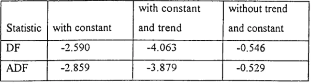
Table 1.3. DF and ADF Tests for Real M oney Balance Using M l and CPI.

Unit root tests for variable LMl-LCPI

DF -2.590 -4.063 -0.546

ADF -2.859 -3.879 -0.529

Unit root tests for variable A(LM1-LCPI)

DF -13.888 -13.858 -13.912

ADF -14.924 -14.857 -14.889

T able 1.4. DF and ADF Tests for R eal M oney Balance Using M l and W PI.

Unit root tests for variable L M l-L W P I

DF -3.057 -3.217 -0.397

ADF -3.362 -3.444 -0.485

Unit root tests for variable A(LM1-LWPI)

DF -13.006 -13.016 -13.055

ADF -13.562 -13.591 -13.605

(35)

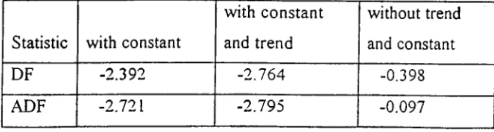
Table 1.5. DF and ADF Tests for Real M oney Balance Using M2 and CPI.

Unit root tests for variable LM2-LCPI

DF -2.392 -2.764 -0.398

ADF -2.721 -2.795 -0.097

Unit root tests for variable A(LM2-LCPI)

DF -9.408 -9.357 -9.444

ADF -6.620 -6.583 -6.655

T able 1.6. DF and ADF Tests for R eal M oney Balance Using M2 and W PI.

Unit root tests for variable LM 2-LW PI

DF -2.418 -2.394 -0.132

ADF -1.428 -1.346 -0.241

Unit root tests for variable A(LM2-LWPI)

DF -8.637 -8.601 -8.681

ADF -7.123 -7.090 -7.164

(36)

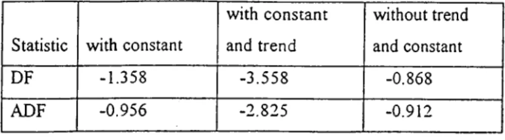
Table 1.7. DF and ADF Tests for Real M oney Balance Using RM and CPI.

Unit root tests for variable LRNI-LCPI

DF -1.358 -3.558 -0.868

ADF -0.956 -2.825 -0.912

Unit root tests for variable A(LRM -LCPI)

DF -10.405 -10.384 -10.377

ADF -10.572 -10.552 -10.538

T able 1.8. DF and ADF Tests for R eal M o n ey Balance Using RM and W PI.

Unit root tests for variable LR M -LW PI

with constant v^athout trend

DF -2.096 -2.841 -0.601

ADF -2.906 -2.841 -0.601

Unit root tests for variable A(LRM -LW PI)

DF -11.043 -11.072 -11.057

ADF -11.043 -11.072 -11.057

(37)

Critical values for the DF test statistics are obtained from Fuller (1976), table 8.5.2. Critical values are the same for both the DF and ADF test statistics and these critical values are presented in Table 2.

T able 2. Critical Values for the DF T e st Statistics for Unit Root Test,

Sample with constant without trend

size = 100 with constant and trend and constant

1% -3.51 -4.04 -2.60

5% -2.89 -3.45 -1.95

10% -2.58 -3.15 -1.61

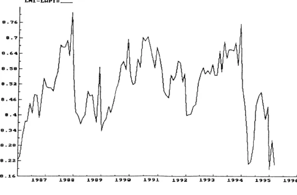
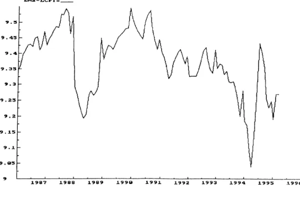
The graphs o f the variables and the graphs o f the first differences o f the variables are presented in the Appendices. In all cases the first differenced series do not exhibit a unit root: the 1(1) hypothesis can only be rejected when the inflation and real money series are first differenced. So according to the DF and ADF test results, real money balances and inflation rate are each integrated o f order one, characterized as 1(1), with test statistics significant even at 1% level.

5 .4 . Testing for Cointegration (Testing for Adaptive Expectations)

The null hypothesis o f no cointegration between inflation and real money balances against one available cointegrating vector is tested using both the Engle and Granger (1987) two-step procedure and Johansen’s (1988) method o f maximum likelihood estimation o f the multi-cointegrated V A R systems.

The Engle-Granger (1987) two-step procedure involves regressing real money balances on inflation rate first, to obtain the residuals. Then the test for the null hypothesis that cointegration exists is based on testing for unit root in the regression residuals using the ADF tests. The results from the cointegrating regressions are presented in Table 3.

(38)

T able 3. Test of C ointegration Betw een Rea! M oney Balances and Inflation Rate. Dependent Variable Independent Variable ADF Statistics LM l-LC PI ALCPI -5.386 LM l-LW PI ALWPI -4.764 LM2-LCPI ALCPI -5.393 LM2-LWPI ALWPI -4.784 LRM-LCPI ALCPI -5.362 LRM-LWPT ALWPI -4.770

ADF test statistics are initially based on regressions with twelve lags. Then a sequential reduction procedure is applied to eliminate the insignificant lagged

differences. The critical values for the ADF test statistics are obtained from Engle and Granger (1987), table 2 and these critical values are presented in Table 4.

T able 4. Critical Values for the A D F T est Statistics for C ointegration Test.

Statistic 1% 5% 10%

ADF -3.77 -3.17 -2.84

Real money balances seem to be cointegrated with inflation rate as ADF test statistics for testing cointegration between real money balances and inflation rate are significant even at 1% level.

All empirical models are inherently approximations o f the actual data generating process and the question is whether the benchm ark model ( 4.3 ) is a satisfactorily close approximation. Therefore we investigated the stochastic specification with respect to residual correlation, heteroscedasticity and normality. The residual tests are reported in Table 5. ov is the standard deviation o f the residuals,

)^(

2

)

is the Jarque-

Bera test statistic for normality, ARCH F(df;6,58) is the ARCH test for heterocedastic

(39)

residuals, AR F(df:6,64) is the test for residual autocorrelation,

skewness

is the third

moment around the mean and

excess kurtosis

is the fourth moment around the mean.

Table 5. Residual M isspecification Tests.

Equation (Js; _X'0 Skew. Ex. kurt. ARCH 6 F AR 1-6F

I A(LMl-LCPI) 0.0523 5.2473 -0.0289 0.8471 2.1576 5.5801 AALCPI 0.0215 71.335 2.6623 12.407 0.0460 0.6436 II A(LM1-LWPI) 0.0520 8.3987 -0.1743 1.2193 3.1029 0.5226 AALWPI 0.0252 95.613 3.2407 18.469 0.0299 1.8788 III A(LM2-LCPI) 0.0212 7.7048 -0.2426 1.1689 0.4264 0.5078 AALCPI 0.0181 44.534 2.4360 13.900 0.0491 0.1359 IV A(LM2-LWPI) 0.0272 4.8235 -0.2228 0.8143 3.0286 2.5585 AALWPI 0.0215 51.185 2.6664 15.210 0.0299 0.8123 V A(LRM-LCPI) 0.0425 4.0534 0.1385 0.7027 1.4039 1.0129 AALCPI 0.0229 81.052 2.9389 15.2843 0.0481 0.7902 VI A(LRM-LWPI) 0.0374 8.7691 0.5873 1.4814 1.1245 0.4862 AALWPI 0.0226 43.956 2.3927 12.8392 0.0445 2.3344

The benchmark model ( 4.3 ) seems to provide a reasonably good approximation o f the data generating process. There is no indication of residual autocorrelation in any o f the series (

F

.99 (6,64)' » 3 .1 2 ) . A RCH 6 F did not reject homoscedasticity o f residuals in any o f the series ( F.99 (6,58) » 3.12 ). A few problems remain, such as

normality o f residuals are rejected for equations o f inflation

{AAp)

no matter which

price index we used ( ;}f.pp(2) = 9.12 ) and first differenced inflation series

{AAp)

(40)

appear to be leptocurtic. Critical values o f F test and chi-square test are obtained from Hines and Montgomery, 1980, table III and V.

Using the procedure suggested by Johansen (1988), cointegration between inflation and real money balances can be investigated by utilizing the VAR model. In

the Johansen (1988) trace test, the null hypothesis is that there are at most

r

cointegrating vectors and it is tested against a general alternative. In the maximum eigenvalue test, the null hypothesis o f

r

cointegrating vectors is tested against

r +

1 cointegrating vectors. The hypothesis o f at most zero and one cointegrating vectors are tested, respectively, and the maximum eigenvalue and the trace test statistics are

presented in Table 6.

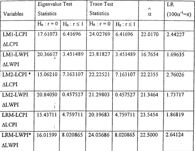
Table 6. Johansen C ointegration Tests an d Estim ates

Variables Eigenvalue Test Statistics Trace Test Statistics A a LR ( 1 0 0 a ‘=7t) Ho : r = 0 H o ; r < 1 Ho ; r = 0 Ho ! r < I LM l-LCPI ALCPI 17.61073 6.41696 24.02769 6.41696 22.0170 2.44227 LM l-LW PI ALWPI 20.3667:7 3.451489 23.81827 3.451489 16.7654 1.69635 LM2-LCPI * ALCPI 15.06210 7.163107 99 99^91 7.163107 22.2355 2.76026 LM2-LWPI ALWPI 20.84050 i 0.457527 21.29803 0.457527 21.3464 1.73717 LRM-LCPI ALCPI 15.43711 4.759711 20.19683 4.759711 23.5454 1.86819 LRM -LW PP ALWPI 16.01599 8.020865 24.03686 8.020865 22.5000 2.64124

* 11 seasonals are included due to the criterion o f equilibrium.

laving a meaningful long run

(41)

The critical values for the trace and maximum eigenvalue test statistics are obtained from Johansen and Juselius (1990), table A2 and these critical values are presented in Table 7.

T able 7. C ritical Values for th e T ra c e a n d M axim um Eigenvalue Test Statistics

Significance 5% Eigenvalue Test Statistics

Ho;

r =

0

14.595

Ho

; r < 1 8.083 Trace Test Statistics Ho : r = 0 17.844 H o ; r < 1 8.083

Applying the trace test and the maximum eigenvalue test for cointegration due to Johansen (1988), the hypothesis o f at most one cointegrating vector ( Ho : r < 1 ) can not be rejected in any case, while the hypothesis o f zero cointegrating vectors ( H o: r = 0 ) is easily rejected in every case. Hence, real money balances and inflation are

cointegrated with the cointegrating vector [1, a ] ( after normalization on real

balances ). This constitutes evidence in favor o f the Cagan model for the Turkish case. So, assuming that agents’ forecasting errors are stationary, the monetary and

inflationary experiences of Turkey can be adequately characterized by the Cagan

(1956) model. Table 6 also lists the estimates o f

a,

which is the cointegrating

parameter after normalization on real balances. The estimates of

a

are calculated by

normalizing the cointegrating vectors, estimated as a result o f Johansen’s cointegration test, on real balances.

j

Cagan (1956) also studied the maximum amount o f revenue that is available from inflation tax. Cagan showed that, in the context o f the hyperinflation model, the

percentage rate o f increase in prices and money, which maximizes the revenue from the inflation tax which results from m oney creation by the authorities, is just equal to (100/a)% . Table 6 also lists the likelihood ratio test statistics for the null hypothesis that 100/a is in fact equal to the average inflation rate which prevailed over the period. The likelihood ratio test statistic, constructed as in Johansen (1988), now becomes

(42)

LR = T Z V iIn { (l n * ) / ( l

-A

where

Hi

are the

r

largest eigenvalues under no restrictions and the /i*, are the

r

largest eigenvalues from solving ( 4.4 ) under the restriction that 100/a is equal to average inflation rate which prevailed over the period. The test statistic is

asymptotically distributed as chi-square with (//-/·) degrees of freedom. In our case,

r

is

equal to one and LR is distributed as chi-square with one degree o f freedom. The critical value for chi-square with one degree o f freedom at 5% level is equal to 3.84 ( Hines and Montgomery, 1980, table III, page 594 ). The hypothesis that the

authorities expanded the money supply, on average, in such a way as to maximize the inflation tax revenue can not be rejected in any case at the 5% level.

5 .5 . Testing the Rational Expectations Hypothesis

I f expectations are formed according to the rational expectations hypothesis, and if following Sargent (1977), we can assume E (^ , | /,) = 0, where

y/t

denotes elements o f money demand not captured by the model as in section III, then the forecasting errors.

= Ap,.i + a ‘(m - p),. ( 5 . 4 )

should be orthogonal to information available at time t, that is

E ( f„ , I/,) = 0. ( 5 . 5 )

A way o f testing (5 .5 ) is to test for zero coefficients in a least squares projection o f ^ ,+ 1 onto lagged values o f itself ( Taylor 1991). Taylor (1991) demonstrates that this is equivalent to testing a set o f cross-equation rational expectations restrictions on

the vector autoregressive representation

oi[A'pt, {(m -p)t

+

aApi)]'.

The test for zero coefficients in a least squares projection o f onto lagged

values o f itself is applied and the results are presented in Table 8. Two sets o f

(43)

forecasting errors, were constructed-one set using the cointegration estimate o f a as reported in Table 6 and one set constructed assuming inflation tax revenue

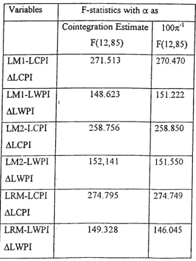
maximization, i.e., with a = 100;r^ Test statistics are distributed as F( 12,85) under the null hypothesis o f rational expectations.

Table 8. Tests o f the H yperinflation M odel Under Rational Expectations

Variables F-statistics with a as

Cointegration Estim ate F(12,85) lOOrr·* F(12,85) LM l-LCPI ALCPI 271.513 270.470 LM l-LW PI ALWPI 148.623 i 151.222 LM2-LCPI ALCPI 258.756 258.850 LM2-LWPI ALWPI 152,141 151.550 LRM-LCPI ALCPI 274.795 274.749 LRM-LWPI ALWPI 149.328 146.045

In all cases the F-statistics are highly significant. In all cases, the results indicate a strong rejection o f the null hypothesis o f rational expectations. So it appears that the Cagan model cannot be coupled with the rational expectations for the Turkish case in the considered period. Note, however, that these results are highly dependent on the assumption that E(

iff,

i

li) -

0, that is on the assumption that expectation o f

iff,

based on information available at time t is equal to zero. Although this assumption has a high degree o f precedent in the hyperinflation literature (see, e.g. Sargent 1977), it is quite arbitrary. If

iff,

is a serially correlated series, then the above assumption w on’t be valid (Taylor and Phylaktis 1991).

(44)

VI - CONCLUSION

Cagan (1956) deals with the relation between changes in the quantity o f money and price level during hyperinflations. The heart o f Cagan’s analysis is a function in which the demand for real balances depends, among other things, inversely on the expected rate o f inflation. Thus, if an expanding supply o f money generates inflation, that inflation lowers the demand for real balances. In the face o f given nominal balances, the price level must rise in order to reduce the supply o f real balances to its demand. Consequently, in hyperinflation, prices rise faster than the nominal supply o f money. Cagan assumes in his model that expectations o f the rate o f inflation are formed adaptively.

This thesis considers the demand for money under conditions o f high inflation in Turkey during the period 1986:1-1995:3. We test whether the monetary and

inflationary experiences of Turkey can be adequately characterized by the Cagan (1956) model, using an econometric procedure which is reliant only on the assumption that forecasting errors ai'e stationary. Although Turkey has not experienced

hyperinflation according to Cagan’s strict definition, Turkey has experienced high rates o f inflation during many years. We first find out that real money balances and inflation are each first difference stationary, or 1(1), using DF and ADF unit root tests. Thus, a simple test o f the applicability o f the hyperinflation model lies in testing whether or not real money balances and inflation are cointegrated and the cointegration test is

conducted using both Engle and G ranger two step approach and Johansen’s cointegration.

Excluding 1994, Turkey has experienced an annual inflation ranging between 60% and 70% in the last decade. Thus w e believe that, in the last decade, the economic agents can have rational expectations for inflation. Having this intuition, we derive a test o f the Cagan (1956) model with the additional assumption o f rational expectations for Turkey for the considered period.

We know that the inflation tax is the tax imposed on money holders as a result o f inflation, or it is the loss in the value o f their real balances. In the thesis, we test the

(45)

hypothesis that the authorities expanded the money supply in such a way as to maximize the inflation tax revenue, in Turkey for the considered period, using a likelihood ratio test statistic constructed as in Johansen (1988).

The results o f this thesis suggest that Cagan’s hyperinflation model does indeed provide an adequate characterization o f the features of the inflationary and monetary experiences o f Turkey for the period 1986:1-1995:3. Moreover, it appears that in the considered period the authorities expanded the money supply in such a way as to maximize the inflation tax revenue. Although we had the intuition that, in the last decade, the economic agents have rational expectations for inflation, it appears that the Cagan model cannot be coupled with the rational expectations hypothesis for Turkey for the considered period.

(46)

Blanchard, O.J. and Fischer, S.,