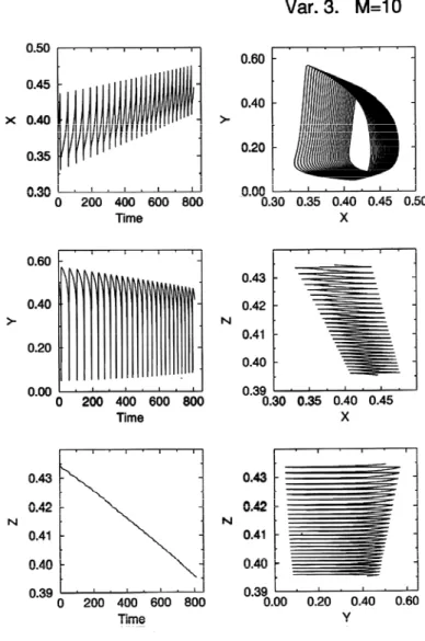
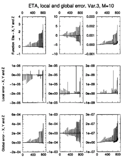
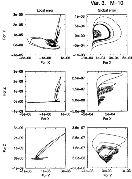
On a global error estimate in long-term numerical integration of ordinary differential equations

Bu noktada, ihraç edilecek menkul kiymetle- rin likiditesinin ve İslami açidan uluslararasi kabul görmüş kriterlere göre seçil- miş menkul kiymetlere dayali yatirim

212 Münevver Dikeç Sonuç olarak, kütüphanecilik ve bilgibilim alanında özellikle bilginin depolanması ve gelecek kuşaklara aktarılmasında CD-ROM yaygın olarak kullanım

ordinary di fferential equation is analyzed on Euler and Runge-Kutta method to find the approximated solution with the given initial conditions.. Then, the

Ulaşılan bu bulgulardan yola çıkarak öğretmenlerin örgütsel adanmışlık düzeyinin kısmen düzeyinde olduğu ve örgütsel adanmışlıklarının orta düzeyde olduğu

Demokratlar bekalarını temin etmek isterlerse tamamiyle Halk Partisinin bu şia­ rına karşı bir siyaset takip etmeleri icap e- der: Bir taraftan komünizme karşı

îbnülemîn Mahmud Kemal İfadedeki mübarek zarafete, te- | lâsla fahriliğe kapamama imkân vermemek hususundaki rikkatleri nasıl mütezahirdir dikkat buyurul­

HFS ve BFS grubunun hastaneye geliş zaman aralığı daha yüksek olarak saptanmasına rağmen diğer gruplar ile karşılaştırıldığında istatistiksel olarak anlamlı farklılık