Power dissipation analysis in tapping-mode atomic force microscopy

Power dissipation analysis in tapping-mode atomic force microscopy

M. Balantekin*and A. Atalar

Bilkent University, Electrical Engineering Department, Bilkent, TR-06800, Ankara, Turkey 共Received 6 February 2003; published 27 May 2003兲

In a tapping-mode atomic force microscope, a power is dissipated in the sample during the imaging process. While the vibrating tip taps on the sample surface, some part of its energy is coupled to the sample. Too much dissipated power may mean the damage of the sample or the tip. The amount of power dissipation is related to the mechanical properties of a sample such as viscosity and elasticity. In this paper, we first formulate the steady-state tip-sample interaction force by a simple analytical expression, and then we derive the expressions for average and maximum power dissipated in the sample by means of sample parameters. Furthermore, for a given sample elastic properties we can determine approximately the sample damping constant by measuring the average power dissipation. Simulation results are in close agreement with our analytical approach.

DOI: 10.1103/PhysRevB.67.193404 PACS number共s兲: 68.37.Ps, 62.25.⫹g

Tapping-mode force microscopy is utilized for surface im-aging at very low lateral forces. The cantilever taps on the sample surface giving rise to the interaction force. This force has two parts: One is the attractive van der Waals 共vdW兲 forces and second is the repulsive Hertzian contact force. These forces pull the sample surface up and down meaning that some part of the cantilever energy is dissipated in the sample where the sample can be modeled with a dashpot and a spring共see Fig. 1兲. If the dissipated power is high enough it can break the bonds of the surface atoms. Therefore, for nondestructive imaging the power dissipation is an important factor to consider. There are several studies1–3which relate the dissipated power to the phase of the cantilever. In this Brief Report we follow a completely different approach: First we obtain an analytical expression of tip-sample inter-action force for a given steady-state tip oscillation amplitude, and then we give the power dissipation in terms of sample parameters. We assume that the higher harmonics of the can-tilever oscillation is negligible, which is usually the case for high-Q systems, and hence the point-mass model describes

the tapping-mode AFM suitably.4In this way we can easily find the dissipated power and compare it with our simulation5result. Moreover, we can find the sample damp-ing constant by measurdamp-ing the average power dissipation.

The tip-sample interaction is highly nonlinear and cannot be solved analytically without doing crude approximations. The simulations are quite useful to interpret experimental observations.5,6 However, the simulations does not give an insight on the effect of overall system parameters. In order to gain further insight, we first need to approximate the nonlin-ear interaction force analytically at a given steady-state tip oscillation amplitude. In a tapping mode, there exist two stable oscillation states.7For the high amplitude solution, the tip-sample interaction force fTShas both attractive and

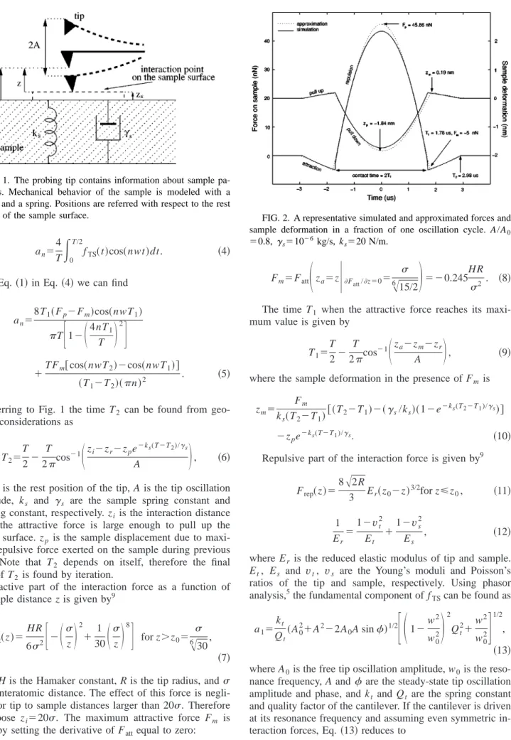
repul-sive parts as shown in Fig. 2. The repulrepul-sive force for 0

⭐兩t兩⬍T1 can be approximated by a cosine. A linear approxi-mation is utilized for the attractive force for T1⭐兩t兩⭐T2. We assume that the force is even symmetric around t⫽0. An analytic expression for the interaction force can be written as

fTS共t兲⫽

冦

F_p⫺F_m 1⫺cos共2␲/␣兲cos

冉

2␲ ␣T1 t

冊

⫹Fm⫺Fpcos共2␲/␣兲 1⫺cos共2␲/␣兲 for 0⭐兩t兩⬍T1 Fm T1⫺T2t⫹ FmT2 T2⫺T1 for T1⭐兩t兩⭐T2 0 for T2⬍兩t兩⭐T/2. 共1兲

In this parametric expression, Fp and Fm are the maximum repulsive and attractive forces exerted on the sample, respec-tively. T is the period of oscillation. ␣ is a fit constant that defines the period of the cosine and its optimum value is different for different oscillation amplitudes. The results for different␣ values are very close to each other and hence for simplicity we choose ␣⫽4. In the steady-state conditions, the periodic interaction force can be represented with a Fou-rier series8

fTS共t兲⫽a0⫹

兺

n⫽1

⬁

a_ncos共nwt兲, 共2兲

where w⫽2␲/T is the oscillation frequency and the series coefficients are a0⫽2 T

冕

0 T/2 fTS共t兲dt, 共3兲 PHYSICAL REVIEW B 67, 193404 共2003兲

an⫽ 4 T

冕

0

T/2

fTS共t兲cos共nwt兲dt. 共4兲

Using Eq.共1兲 in Eq. 共4兲 we can find an⫽ 8T1共Fp⫺Fm兲cos共nwT1兲 ␲T

冋

1⫺

冉

4nT1 T

冊

2

册

⫹TFm关cos共nwT2兲⫺cos共nwT1兲兴 共T1⫺T2兲共␲n兲2 . 共5兲

Referring to Fig. 1 the time T2 can be found from

geo-metric considerations as T2⫽T 2⫺ T 2␲cos ⫺1

冉

zi⫺zr⫺zpe⫺ks(T⫺T2)/␥s A

冊

, 共6兲

here z_r is the rest position of the tip, A is the tip oscillation amplitude, ks and ␥s are the sample spring constant and damping constant, respectively. zi is the interaction distance where the attractive force is large enough to pull up the sample surface. zp is the sample displacement due to maxi-mum repulsive force exerted on the sample during previous cycle. Note that T2 depends on itself, therefore the final

value of T2 is found by iteration.

Attractive part of the interaction force as a function of tip-sample distance z is given by9

Fatt共z兲⫽HR 6␴2

冋

⫺

冉

␴ z

冊

2 ⫹₃₀1

冉

␴_z

冊

8

册

for z⬎z0⫽ ␴

冑

6 30, 共7兲

where H is the Hamaker constant, R is the tip radius, and␴ is the interatomic distance. The effect of this force is negli-gible for tip to sample distances larger than 20␴. Therefore we choose z_i⫽20␴. The maximum attractive force F_m is found by setting the derivative of Fattequal to zero:

Fm⫽Fatt

冉

za⫽z

冏

⳵F_att/⳵z⫽0⫽ ␴

冑

6 15/2

冊

⫽⫺0.245 HR ␴2 . 共8兲

The time T1 when the attractive force reaches its

maxi-mum value is given by

T1⫽T 2⫺ T 2␲cos ⫺1

冉

za⫺zm⫺zr A

冊

, 共9兲

where the sample deformation in the presence of Fmis

z_m⫽ Fm ks共T2⫺T1兲 关共

T2⫺T1兲⫺共␥_s/k_s兲共1⫺e⫺ks(T2⫺T1)/␥s兲兴 ⫺zpe⫺ks

(T_⫺T1)/␥_{s. 共10兲}

Repulsive part of the interaction force is given by9

Frep共z兲⫽8

冑

2R 3 Er共z0⫺z兲 3/2_{for z⭐z} 0, 共11兲 1 E_r⫽ 1⫺v_t2 E_t ⫹ 1⫺v_s2 E_s , 共12兲

where Er is the reduced elastic modulus of tip and sample. Et, Es and vt, vs are the Young’s moduli and Poisson’s ratios of the tip and sample, respectively. Using phasor analysis,5the fundamental component of fTScan be found as

a1⫽kt Qt共A0

2_⫹A2_{⫺2A0A sin␾兲}1/2

冋冉

_1⫺w 2 w₀2

冊

2 Qt 2_⫹w 2 w₀2

册

1/2 , 共13兲

where A0is the free tip oscillation amplitude, w0is the

reso-nance frequency, A and␾ are the steady-state tip oscillation amplitude and phase, and kt and Qt are the spring constant and quality factor of the cantilever. If the cantilever is driven at its resonance frequency and assuming even symmetric in-teraction forces, Eq.共13兲 reduces to

FIG. 1. The probing tip contains information about sample pa-rameters. Mechanical behavior of the sample is modeled with a dashpot and a spring. Positions are referred with respect to the rest

position of the sample surface. _{FIG. 2. A representative simulated and approximated forces and}

sample deformation in a fraction of one oscillation cycle. A/A0

⫽0.8, ␥s⫽10⫺6 kg/s, ks⫽20 N/m.

BRIEF REPORTS PHYSICAL REVIEW B 67, 193404 共2003兲

a1⫽kt Qt共A0

2_⫺A2_兲1/2_{. 共14兲}

Fp and zr must satisfy the following equations simulta-neously: a1⫽8T1共Fp⫺Fm兲cos共wT1兲 ␲T

冋

1⫺

冉

4T1 T

冊

2

册

⫹TFm关cos共wT2兲⫺cos共wT1兲兴 ␲2_{共T1⫺T2兲} , 共15兲 Fp⫽ 8

冑

2R 3 Er共z0⫺zr⫹A⫺zp兲 3/2_{, 共16兲}

where the sample displacement when Fp is exerted on the sample is zp⫽ F_p ks⫹

冉

zm⫺ F_m ks

冊

e⫺ksT1/␥s ⫹␥s共Fm⫺Fp兲共1⫺e⫺ksT1/␥s兲 k_s2T1 . 共17兲

The displacement of the sample surface due to fTSis

gov-erned by the following differential equation

␥s dz_s共t兲

dt ⫹kszs共t兲⫽ fTS共t兲, 共18兲

using superposition, we can add the displacements due to different frequencies to get the total displacement

zs共t兲⫽ a0 ks ⫹

兺

n⫽1 ⬁ _a n

冑

k_s2⫹共nw␥s兲2 cos

冋

nwt⫺tan⫺1

冉

nw␥s ks

冊册

. 共19兲

The instantaneous power dissipated in the sample is given by

p共t兲⫽ fTS共t兲dzs共t兲

dt . 共20兲

If we integrate p(t) over one cycle and divide by the period, we get the average power. Hence we obtain our final result

Pavg⫽

兺

n⫽1 ⬁ _a n 2 2

冑

␥_s2⫹共ks/nw兲2 sin

冋

tan⫺1

冉

nw␥s ks

冊册

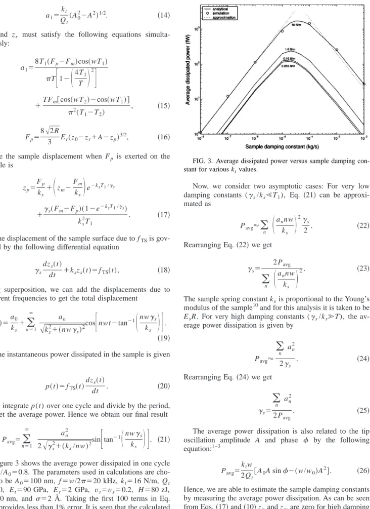
. 共21兲 Figure 3 shows the average power dissipated in one cycle for A/A0⫽0.8. The parameters used in calculations are

cho-sen to be A0⫽100 nm, f ⫽w/2␲⫽20 kHz, kt⫽16 N/m, Qt

⫽250, Et⫽90 GPa, Es⫽2 GPa, vt⫽vs⫽0.2, H⫽80 zJ, R⫽10 nm, and ␴⫽2 Å. Taking the first 100 terms in Eq.

共21兲 provides less than 1% error. It is seen that the calculated

and the simulated power values are in agreement.

Now, we consider two asymptotic cases: For very low damping constants (␥s/ksⰆT1), Eq. 共21兲 can be approxi-mated as Pavg⬇

兺

n

冉

a_nnw ks

冊

2_␥ s 2 . 共22兲

Rearranging Eq. 共22兲 we get

␥s⫽ 2 Pavg

兺

n

冉

annw ks

冊

2. 共23兲

The sample spring constant ksis proportional to the Young’s modulus of the sample10and for this analysis it is taken to be E_sR. For very high damping constants (␥_s/k_sⰇT), the av-erage power dissipation is given by

Pavg⬇

兺

n

a_n2

2␥_s . 共24兲

Rearranging Eq. 共24兲 we get

␥s⫽

兺

n

a_n2

2 Pavg

. 共25兲

The average power dissipation is also related to the tip oscillation amplitude A and phase ␾ by the following equation:1–3

Pavg⫽ktw

2Q_t关A0A sin␾⫺共w/w0兲A

2_{兴. 共26兲}

Hence, we are able to estimate the sample damping constants by measuring the average power dissipation. As can be seen from Eqs.共17兲 and 共10兲 zpand zmare zero for high damping constants, and they are equal to Fp/ks and Fm/ks for low

FIG. 3. Average dissipated power versus sample damping con-stant for various ktvalues.

BRIEF REPORTS PHYSICAL REVIEW B 67, 193404 共2003兲

damping constants, respectively. Equations共22兲 and 共24兲 are also plotted in Fig. 3. The approximation is valid for either low or high damping constants, it deviates from the exact result for medium␥svalues.

The procedure to find ␥s for a sample with known elas-ticity can be stated as follows. First, the interaction force parameters are found using Eqs. 共6兲–共17兲. Using Eq. 共5兲 an values are calculated. The average power given by Eq. 共26兲 is determined. Finally,␥_svalues are found using Eqs.共23兲 or

共25兲. AMATLABcode that does these calculations is available for download.11

To calculate the error bounds, we made several simula-tions. Table I summarizes the results. The Hamaker constant H depends on tip-sample system geometry, and the tip radius R can roughly be estimated. Therefore we include the errors coming from these constants into our analysis. It is seen that the phase measurement error in P_avgis dominant. Also, it is interesting to see that adding a 50% uncertainty to H or R does not significantly alter the results.

To find the maximum power dissipation, we equate d2zs(t)/dt2 to zero and get

t⫽ 1

nw

冋

␲/2⫹tan

⫺1

冉

nw␥s ks

冊册

. 共27兲

Substituting Eq.共27兲 into Eq. 共20兲 we get

Pmax⫽

兺

n an

冑

␥s 2_⫹共k s/nw兲2

兺

n ansin

冋

tan⫺1

冉

nw␥s ks

冊册

. 共28兲

Although the average power dissipation is in femtowatt lev-els, we have to consider the peak power dissipated in the sample. It is found that the peak instantaneous power can be more than 100 times the average power.

In summary, we formulated the average and maximum power dissipation in terms of the sample parameters. This analytical approach also gives a physical meaning to the phase␾ of the cantilever关see Eqs. 共21兲 and 共26兲兴. It is clear that ␾ is a complicated function of the tip and the sample parameters as well as the oscillation amplitude. In addition, we are able to find many important quantities such as the contact time, the sample deformation, and the maximum forces exerted on the sample analytically. We also see from Fig. 3 that softening the lever more and more does not sig-nificantly reduce the power dissipation which is not seen directly from Eq. 共26兲.

*Email address: [email protected]

1_{J. Tamayo and R. Garcia, Appl. Phys. Lett. 73, 2926共1988兲.} 2_{J. P. Cleveland, B. Anczykowski, A. E. Schmid, and V. B. Elings,}

Appl. Phys. Lett. 72, 2613共1998兲.

3_{B. Anczykowski, B. Gotsmann, H. Fuchs, J. P. Cleveland, and V.}

B. Elings, Appl. Surf. Sci. 140, 376共1999兲.

4_{T. R. Rodriguez and R. Garcia, Appl. Phys. Lett. 80, 1646共2002兲.} 5_{M. Balantekin and A. Atalar, Appl. Surf. Sci. 205, 86共2003兲.}

6_{O. Sahin and A. Atalar, Appl. Phys. Lett. 78, 2973共2001兲.} 7_{R. Garcia and A. SanPaulo, Phys. Rev. B 61, R13 381共2000兲.} 8_{R. W. Stark and W. M. Heckl, Surf. Sci. 457, 219共2000兲.} 9_{M. Hoummady, E. Rochat, and E. Farnault, Appl. Phys. A: Mater.}

Sci. Process. 66, S935共1998兲.

10_{R. G. Winkler, J. P. Spatz, S. Sheiko, M. Mo¨ller, P. Reineker, and}

O. Marti, Phys. Rev. B 54, 8908共1996兲.

11_{URL: www.ee.bilkent.edu.tr/⬃mujdat}

TABLE I. Actual and estimated␥svalues. Estimated␥swith

10% error included in 50% error included in

Multiplying

factor Actual␥s Estimated␥s H R Pavg H R Pavg

10⫺8 1.00 1.04 1.04⫾0.02 1.04⫾0.02 1.04⫾0.11 1.05⫾0.12 1.06⫾0.13 1.04⫾0.53 10⫺7 1.00 1.04 1.04⫾0.02 1.04⫾0.02 1.04⫾0.11 1.05⫾0.12 1.06⫾0.13 1.04⫾0.53 10⫺6 1.00 1.01 1.01⫾0.02 1.01⫾0.02 1.01⫾0.10 1.01⫾0.12 1.02⫾0.13 1.01⫾0.50 10⫺5 1.00 0.77 0.77⫾0.02 0.77⫾0.02 0.77⫾0.08 0.78⫾0.09 0.78⫾0.10 0.78⫾0.39 10⫺4 1.00 1.36 1.36⫾0.03 1.34⫾0.05 1.37⫾0.14 1.36⫾0.10 1.32⫾0.23 1.81⫾0.90 10⫺3 1.00 0.78 0.78⫾0.02 0.79⫾0.03 0.78⫾0.08 0.78⫾0.06 0.78⫾0.14 1.06⫾0.54 10⫺2 1.00 0.76 0.76⫾0.04 0.77⫾0.03 0.76⫾0.08 0.76⫾0.06 0.76⫾0.13 1.00⫾0.50

BRIEF REPORTS PHYSICAL REVIEW B 67, 193404 共2003兲