Robust regression, HCCM estimators, and an Empirical Bayes application

(1)

(2)

ROBUST REGRESSION, H C C M ESTIM ATOR S, A N D A N EM PIRICAL BAYES A PPLIC ATIO N

A THESIS PRESENTED BY MEHMET ORHAN TO

THE INSTITUTE OF

ECONOMICS AND SOCIAL SCIENCE^ IN PARTIAL FULFILLMENT OF THE

REQUIREMENTS

FOR THE· DEGREE OF Ph. D. OF ECONOMICS

BILKENT UNIVERSITY May, 1999

(3)

ИА

3 4 3

' 0 ? 4

(4)

I certify that I have read this thesis and in my opinion it is fully adequate, in scope and in quality, as a thesis for the degree of Ph. D. o f Economics.

Prof. Dr. Asan Mman

I certify that I have read this thesis and in my opinion it is fully adequate, in scope and in quality, as a thesis for the degree o f Ph. D. of Economics.

ssist. Prof. Dr. Mehmet Caner

I certify that I have read this thesis and in my opinion it is fully adequate, in scope and in quality, as a thesis for the degree of Ph. D. of Economics.

Assist. Prof. Dr. Savaş Alpay

Assist. Prof. Dr. Siiheyla Ozyildirim

Assoc. Prof. Dr. Turan Erol

(5)

A B S T R A C T

ROBUST REGRESSION, HCCM ESTIM ATORS, AND AN EMPIRICAL BAYES APPLICATION

MEHMET ORHAN Ph. D. OF ECONOMICS Supervisor: Prof. Dr. Asad Zaman

May 1999

This Ph.D. thesis includes three topics o f econometrics where the chapters of the whole study are devoted to robust regression analysis, research on the estimators for the covari ance matrix of a heteroskedastic regression and finally an application of the Empirical Bayes method to some real data from Istanbul Stock Exchange. Some robust regression techniques are applied to some data sets to show how outliers of a data set may lead to wrong inferences. The results reveal that the former studies have gone through some wrong results with the effect o f the outliers that were not detected. Second chapter makes a thorough evaluation o f the existing heteroskedasticity consistent covariance matrix esti mators where the Maximum Likelyhood estimator recently promoted to the literature by Zaman is also taken into consideration. Finally, some empirical study is carried out in the last part of the thesis. The firms o f ISE are categorized into sectors and some estimation is done over an equation which is very common and simple in the finance literature.

Key Words: Heteroskedasticity, Breakdown Point, Least Median of Squares, Outlier, Robust Distance, Empirical Bayes.

(6)

Ö ZET

KATI REGRESYON, HUKM TAHMİN EDİCİLERİ, VE BİR AMPİRİK BAYES UYGULAM ASI

MEHMET ORHAN Doktora Tezi, İktisat Bölümü Tez Yöneticisi: Prof. Dr. Asad Zaman

May 1999

Bu doktora tezi üç ekonometri konusunu içermektedir ki bunlardan ilki katı regresyon analizine, İkincisi heteroskedastik regresyonda kovaryans vektörü tahmin edicileriyle ilgili araştırmalara, ve sonuncusu da İstanbul Borsası’ndaki gerçek verilerin kullanıldığı Am pirik Bayes yöntemine ayrılmıştır. Değişik katı regresyon teknikleri avantajlı ve sakıncalı taraflarıyla incelenmiş ve katı regresyon analizinin katkılarıyla daha önceden yapılmış bazı çalışmalar gözden geçirilmiştir. Sonuçlar ortaya çıkarmıştır ki daha önceki çalışmalarda dikkate alınmayan bazı dışgözlemler yanlış neticelere yol açmışlardır. İkinci kısım, mev cut heteroskedastisitiye uygun kovaryans matrisi (HUKM)tahmin edicilerinin teferruatlı ve kapsamlı bir değerlendirmesini bazı karşılaştırma kriterlerine göre yapmıştır. Zaman tarafından literatüre kazandırılan bir tahmin edici de dikkate alınmıştır. Son olarak, am pirik bir çalışma yapılmıştır. İstanbul Borsası’ndaki firmalar sektörlere sınıflandırılmış ve bunlar üzerinde finans literatüründe çok yaygın ve basit bir denklem kurularak bazı katsayı vektörü tahminleri yapılmıştır.

Anahtar Kelimeler: Heteroskedastiklik, Kırılma Noktası, En Küçük Kareler Medyanı, Dışgözlem, Katı Mesafe, Ampirik Bayes.

(7)

Acknowledgements

I would like to express my gratitude to Prof. Dr. Asad Zaman for his valuable supervision and for providing me with the necessary background in econometrics. Special thanks go to Assist. Prof. Erdem Başçı for his helps and advices throughout my Ph.D. studies. I also would like to thank professors Turan Erol, Savctş Alpay, Mehmet Caner, and Süheyla Ozyıldırım for their valuable comments, and contributions as the members o f the jury and Kıvılcım Metin and Kıvanç Dinçer who kindly accepted to be the members o f the evaluation committee. I also thank my wife, Zeynep, and my little son Mustafa Fethi, although he has done nothing else than smiling.

(8)

1 Robust Regression Analyses with Applications

1.1 Introduction

One might expect to see some reasonable and realistic results even when some of the data points deviate from the usual assumptions o f classical regression analysis, but the classical regression method is very sensitive to the outliers. Indeed, the least squares method is currently the most popular approach for estimation. There are several reasons for this, two of which are the ease of calculation and the tradition that shaped the current literature.

Real data sets containing outliers are very common situations. So many data sets con tain outliers as a result o f mistakes in recording or observing the data or some exceptional observations that might take place. It is possible that the estimates become totally incor rect and the outliers themselves are hidden, which means that it becomes impossible to detect the existence of the outliers for ever. To solve this problem out, robust statistical techniques (RRT) ^ have been developed. These techniques give more trustworthy results when the data are contaminated and may let us identify the outliers to some extend.

The goal of positive breakdown regression is to be robust against the possibility o f one or more unannounced outliers that may be seen anywhere in the data. The outliers may be in the response variable as well as the regressors themselves. The positive breakdown regression became more popular in the eighties although there was a huge amount o f previous work about the detection and the neutralization of the outliers via different methods that have their own positives and negatives.

Let’s suppose that we have a simple linear regression model:

Vi — Po + + · . . + Pk^ik + ₍

1

₎

for i = l ,2, . .., n where y stands for the response variable (dependent variable) and x stands for the independent regressors (explanatory variables). Po denotes the constant term, or the vertical intercept. The classical theory assumes that the error term, e follows a Gaussian distribution with mean 0 and variance cr^. The main objective is to make some inferences about the vector of coefficients, /3. The Ordinary Least Squares (OLS) residual

(11)

for the row o f observations, Cj, is given by

/^1) · · · , /5fc) —

yi

(^0) · · · )

^k^ik)

(2)

More precisely speaking, the objective o f the LS method is to minimize the sum o f squares o f the residuals e i{0 o ,$ i,... ,Pk)· More formally.

minimize

n

{PoA

..

Pk)

i=l

(3)

The main idea is to make all of the residuals as small as possible so that the sum o f their squares should be minimized. Indeed, the observations that deviate from the bulk o f the data are penalized by taking the square of the distance from the line. LS simply wants to place a line among the regression points in such a way that the cumulative squares of the distances is minimized. The main motivation behind such a preference is that the method lets one to compute the vector o f coefficients directly and explicitly from the data by a simple formula.

After such an initiation Gauss was able to introduce the distribution which is world famous by his name, the Gaussian distribution, as the one for which LS is optimal. More recently, people began to realize that actual data often do not satisfy his assumptions, sometimes with dramatic deviations from them leading to some serious mistakes of the estimation procedure.

In the terminology, regression outliers are observations that do not obey the linear pattern formed by the majority of the data. It is difficult to make a good analysis of how things are shaped for robust regression because the mentioned outliers do usually affect the trend of the data in such a way that one can never be sure about the whole picture without working on the outliers. In most cases outliers are not the mistakes but they are the cases which represent the data coming from extraordinary conditions. But some recording or reading errors o f the data are also possible. Regardless of the source of the outliers the conclusion is that one has to detect and work on them very carefully to make some correct inferences.

We say that an observation {xi^yi) is a leverage point when its regressor lie outside of the majority o f the regressors. Indeed, the term leverage comes from mechanics, because

(12)

such a point pulls the LS solution towards it. The LS method estimates a from the residuals, ej using the formula:

1

n - fc - 1 5_i=l

(4)

where k is apparently the number of regressors. Once the estimate for variance is calculated one can obtain the standardized residuals, ef/a . It is also common to calculate these values and label the observations for which this figure exceeds 2.5, or less than -2.5 as the regression outliers. The logic behind is that values generated by Gaussian Distribution are rarely larger than 2.5 or less than -2.5, whereas the other observations are considered to obey the model. In simple regression models, where the number o f regressors is small, the detection o f the outliers may be possible even by observing the plot of the regressors and the regressand, but in multiple regression, where k is large, the detection by eye is no longer possible and the residual plot mentioned about above become an important tool. Since most o f the regressions done by the economists and even the econometricians are done routinely, many results must have been affected or even determined by the outliers and this may have remained unnoticed.

1.1.1 Breakdown Value

In any data set, one can displace the LS fit as much as he wants by simply moving a single data point {xi^Vi) enough far away. This statement can be experimented by any statistical package by changing one of the observations. The statement is true for both single and multiple regression. On the other hand, it is possible to find some robust regression methods that can resist some of the outliers.

The breakdown value can be considered as a superficial but useful measure. The concept was first introduced by Hampel [34] and is applied to the finite sample setting by Donoho and Huber [21]. It is a rough but useful measure of robustness. Let’s use the latter

version. Consider a data set Z = {x n^. . . , ^ = 1? · · · ? ^) and a regression estimator ET. Applying ET to Z yields a vector o f regression coefficients.

Now consider all possible contaminated data sets Z ' obtained by replacing any m of the original observations by arbitrary points.

(13)

This yields the maximum bias

Tnaxbias{m·, ET, Z) := m axz’ \ET{Z') — ET(Z)\

₍₅₎

where | . | is the Euclidean norm. If m outliers can have an arbitrarily large effect on ET, it follows that maxbias{m; ET^ Z) = oo, hence E T (Z ’ ) becomes useless. Therefore, the breakdown value o f the estimator ET at the data set Z is defined as

rTTl

e^{ET^Z) := m in {—\maxbias[m\ET^Z) = 00}

n (6)

In other words, it is the smallest fraction of contamination that can cause the regression method ET to run away arbitrarily far from E T (Z). For many estimators e* (F?T, Z) varies only slightly with Z and n, so that we can denote its limiting value (for n 00) by e*{ET).

How does the notion of breakdown value fit in with the use of statistical models such as (1)? We essentially ajssume that the data from a mixture of which a fraction (1 — e) was generated according to (1), and a fraction e is arbitrary (it could even be deterministic, or generated by any distribution). In order to be able to estimate the original parameters (/3o,. . . we need that e < e*{ET), For this reason e* is sometimes called breakdown bound.

For least squares we know that one outlier may be sufficient to destroy the regression. Its breakdown value is thus e*(£JT, Z ) = 1 /n hence e*{ET) = 0. The estimators where

e*{ET) > 0, will be called positive-breakdown methods.

1.1.2 Positive-Breakdown Regression

Let us first consider the simplest case (k=0) in which the model (1) reduces to a univariate location problem yi = /?o + The LS method (3) yields the sample average ET =

Pq = Ei{yi), E standing for the expected value or the average, with again e*(ET) = 0%. On the other hand, it is easily verified that the sample median ET := medi{yi) has

e*{ET) = 50%, which is the highest breakdown value attainable. Because for a larger fraction of contamination, no method can distinguish between the original data and the replaced data. The further the contamination is disseminated, the worse the situation is. Estimators ET with e*{ET) = 50%, like the univariate median, will be called

(14)

high-breakdown estimators.

The first high-breakdown regression method was the repeated median estimator pro posed by Siegel [92] in 1982. It computes univariate medians in a hierarchical way. For simple regression, it is described in the entry Repeated Median Line Method. Its asymp totic behaviour was obtained by Hossjer et al [43], and for algorithms and numerical results see Rousseeuw et al [83, 85]. But in multiple regression where {k > 2) the repeated median estimator is not equivariant, in the sense that it does not transform properly under linear transformations o f [x n^. . . , Xik)·

However, it is possible to construct a high-breakdown method which is still equivariant. It is instructive to look at (3). This criterion should logically be called least sum of squares, but for historical reasons (Legendre’s terminology) the word sum is rarely mentioned. Now let us replace the sum by a median. This yields the least median of squares method (LMS), defined by

minimize 0^ ^jnedirf

(7)

[78] which has a 50% breakdown value. The LMS is clearly equivariant because (7) is based on residuals only.

Another method is the least trimmed squares method (LTS) proposed in (Rousseeuw [76, 78]). It is given by

h

minimizcp^ 0^

: n (8)

i=l

where (r^)l : n < (r^)2 : n < {r^ )n :n axe the ordered squared residuals (note that the residuals are first squared and then ordered). Criterion 8 resembles that o f LS but does not count the largest squared residuals, thereby allowing the LTS fit to steer clear of outliers. For the default setting h « n /2 we find e* = 50%, whereas for larger h we obtain €* « (n — h)In. For instance, putting h « 0.75n yields e* = 25%, which is often sufficient. The LTS is asymptotically normal unlike the LMS, but for n < 1000 the LMS still has the better finite-sample efficiency. Here we will focus on the LMS, the LTS results being similar.

When using the LMS regression, o can be estimated by

5

(15)

where n are the residuals from the LMS fit, and 1.483 = i>“ ^(3/4) makes a consistent at Gaussian error distribution. The finite-sample correction factor ^1 + ) was obtained from simulations. Note that the LMS scale estimate a is itself highly robust. Therefore, we can identify regression outliers by their standardized LMS residuals ri/a.

In regression analysis inference is very important. The LMS by itself is not suited for inference because of its low finite-sample efficiency. This can be resolved by carrying out a reweighted least squares, RLS, step. To each observation i one assigns a weight Wi

based on its standardized LMS residual n / d , e.g. by putting wi := w{\ri/a\) where w is a decreasing continuous function. A simpler way that is followed in this study many times, but still eflFective, is to put wi if |Tila\ < 2.5 and Wi = 0, otherwise. But simplicity brings some trouble of not qualifying the point as a good leverage one. Either way, the RLS fit (/?o, A , /?2, · · ·, A ) is then defined by:

.... (10)

i=l

which can be computed quickly. The result inherits the breakdown value, but is more efficient and yields all the usual inferential output such as t-statistics, F-statistics, and statistics, and the corresponding p-values. The p-values assume that the data with

Wi = 1 come from the model (1) whereas the data with Wi = 0 do not. Another approach which avoids this assumption is to bootstrap the LMS, as done by Efron and Tibshirani [23]. The LMS and the RLS are computed with the program PROGRESS by Rousseeuw and Leroy [84]. Indeed, the RLS does nothing more than running OLS over the data set avoiding the observations with 0 weights assigned by LMS.

1.1.3 Detecting Leverage Points by Eye

In the typical regression model a data point {xn,Xi2,. . . ,Xih^Vi) with outlying

Xi{xii^Xi2^ · · · T^ik) plays a crucial role, because a slight change of the coefficients estimated may give case i a large residual. Therefore, the LS method gives priority to approaching such a point in minimizing the objective function.

Detecting outliers in the k-dimensional data set X is not trivial. Especially where k is greater than two when we can no longer have the opportunity o f inspection by eye.

(16)

A classical approach to the solution of the problem is to compute the Mahalanobis Distance defined as:

M D {xi) = sj{xi - X ){C o v {X ))-^ {x i - X y

₍

₁₁

₎

for each rcf. Here X is the sample mean of the data set where the C ov{X ) is the sample covariance matrix. This distance tells us how far away xi from the mass o f the data relative to the size of the mass is. It is well known that this approach suffers from the masking effect, by which the multiple outliers do not necessarily have a large Mahalanobis Distance.

One of the most commonly used statistic to discover the leverage points has been the diagonal entries o f the hat matrix. Indeed, these entries are equivalent to the Mahalanobis Distances since.

M D l 1 , ,

ha —---r H— (12)

n — 1 n

Therefore, the diagonal entries of the hat matrix are masked when the distances are masked.

One can play with the elements in the square root formula o f the (11) equation to have some more reliable diagnostics.

The Minimum Volume Ellipsoid proposed by Rousseeuw [77, 79] proposes an ellipsoid with the minimum volume to include some certain percentage of the data. One can refer to [84] in order to have some more detailed information about the technique.

Since the MVE estimator, the robust distances RD{xi) and the one-step reweighted estimates (14) depend only on the x-data, they can also be computed in data sets without a response variable yi. This makes them equally useful to detect one or several outliers in an arbitary multivaraite data set. For some examples see [86], page 634, and [10].

The MVE and the R D {xi) can be computed by the software available from the super visor or the author of this thesis, as well as the LTS subroutine written in Gauss.

(17)

1.1.4 D ia g n o stic D isp lay

Combining the notions of regression oultliers and leverage points, we see that four types o f observations may occur in regression data:

regu la r o b serv a tion s with internal Xi and well-fitting yi

v e rtica l ou tliers with internal Xi and non-fitting yi

g o o d leverage p o in ts with outlying Xf and well-fitting yi

b a d leverage p o in ts with outlying Xi and non-fitting yi

In general, good leverage points are beneficial, since they can improve the precision of regression coefficients. Bad leverage points are harmful because they can change the least squares fit drastically. In the coming applications one o f the best techniquies is to detect the regeression outliers with standardized LMS residuals and leverage points which are diagnozed by robust distances. Indeed, Rousseeuw and van Zomeren proposed a display which plots robust residuals versus robust distances [87] where the cutoffs at the [-2.5,2.5] band and the 0.975 are bordered by horizontal and vertical lines. W ith the help o f such a display, the four types of points categorized above are determined automatically. One can play with the band length and the critical values o f the to be more robust or loose to such points of outliers.

1.1.5 A p p lica tio n s

Although there are some applications of positive-breakdown methods, there have been quite a few substantive applications performed where the use of LMS and/or M VE has made a difference.

The main obstacle preventing the wide, common, and frequent applications of high breakdown methods was the difficulty and slowness of computation, but the invention of powerful computers enabled such computations available. For instance, there are several intensive users of LMS in financial markets, where profits can be made by finding majority patterns and detecting subgroups that believe in another way. In management science, the LMS has been applied to measures o f production efficiency by Seaver and Trinatis

(18)

[91]. The LMS regression is being used in chemistry after the publication o f Maissart et al [66]. Also, the LMS is an essential component o f a new system for connecting optical fiber cables implemented at NIST, see Wang et al [106]. In large electric power systems, Mili et al [70] modified positive-breakdown methods to estimate the system’s state variables. Faster algorithms needed to be constructed to allow real-time estimation.

Positive-breakdown methods have opened new possibilities in the rapidly evolving field of computer vision. The LMS has been used for analyzing noisy images, Meer et al [68], for interpreting color omages Drew [22], for discontinuity-preserving surface reconstruction, Sinha and Schunk [95], for extracting geometric primitives, Roth and Levine [75], Stewart [99], for robot positioning Kumar and Hanson [53], and for detecting moving objects in video from a mobile camera, Thompson et al [104], Abdel-Mottaleb et al [1]. The MVE was applied to image segmentation Jolion et al [46]. Chork [10] used the MVE to analyze data on surface rocks in New South Wales, for which concentrations o f several chemical elements were measured. Outliers in this multivariate data set revealed mineralizations, yielding targets for mining prospection. A larger study in Finland carried out MVE-based factor analysis, Chork and Salminen [11]. The same methods apply to environmetrics, since mineralizations in geochemistry are similar to contaminations o f the environment.

1.1.6 Other Robust Methods

The earliest systematic theory o f robust regression was based on M-estimators Huber [44], [45] given by

n

minimize I a) (13)

¿=1

where p{t) = [tj yields regression (see Method of Least Absolute Values) as a special case. For general p one needs a robust a to make the M-estimator equivariant under scale factors. This d either needs to be fixed in advance or estimated jointly with (/?o, · . . , /3^;), see Huber [45], page 179. Scale equivariance holds automatically for R-estimators, Jureckova [49], and L-estimators Koenker and Portnoy [52]. The breakdown value o f all M-, L-, and R- estimators is 0% because of their vulnerability to bad leverage points.

Zaman [112] makes a thorough appreciation of the robust methods where he mentions the need for the consequently invented estimators, with the drawback o f them in chapter

(19)

The next step was the development of generalized M-estimators (GM- estimators) with the purpose of bounding the influence of outlying {x n^, . . ,Xik) by giving them a small weight. This is why GM-estimators are often called bounded influence methods. A survey is given in Hampel et al [35]. Both M- and GM-estimators can be computed by iteratively rewighted LS or by the Newton-Raphson algorithm. Unfortunetly the breakdown value o f all GM-estimators goes down to zero for increasing k, when there are more opportunities for outliers to occur.

In the special case o f simple regreesion (k = l) several earlier methods exist, such as the Brown-Mood line, the robust-resistant line of Tukey, and the Theil-Sen slope. Their breakdown values are derived in Rousseeuw and Leroy ([84] Section 2.7).

For multiple regression the LMS and the LTS described above were the first equivariant methods to attain a 50% breakdown value. By choosing h in (8), any positive breakdown value between 0% and 50% can be set as well. Their low finite-sample efficiency can be improved by carrying out one-step RLS fit (10) afterwards. Another approach is to compute one-step M-estimators starting from LMS as proposed by Rousseeuw [78], which also maintains the breakdown value and yields the same asymptotic efficiency as the corresponding M-estimator. In order to combine these advantages with those o f the bounds influence approach, it was later proposed to follow the LMS or LTS by a one-step GM- estimator of the Mallows type, see Simpson et al [93], the Schweppe type, see Coakley and Hettmansperger [13], or the Hill-Ryan type, see Simpson and Yohai [94]. For tests and variable selection in this context see Markatou and He [59] and Ronchetti and Staudte [74].

A different approach to improving on the efficiency of the LMS and the LTS is to replace their objective functions by a more efficient scale estimator applied to the residuals r^. This yielded the class of S-estimators, see Rousseeuw and Yohai [89]. An S-estimator is the (^0, · · ·) 0k) which minimizes an M- estimator S' (ri , . . . , r^) given by

ri \

5.

1 ^

(14)

with bounded p. The breakdown value of the S-estimator . .. ,Pk) depends on k and n, and can be as high as 50%. Altough S-estimators are not M- estimators, they happen to

(20)

have the same expression for their influence function, hence they have the same asymptotic efficiency. Anologuous situations already occur in univariate location where the trimmed mean L-estimator and the Huber-type M-estimator happen to possess the same infuence function while their breakdown values are different.

Going further in this direction has led to the introduction of even more efficient positive- breakdown regression methods, including MM-estimators, Yohai [110], r-estimators , Yohai and Zamar [111], and generalized S-estimators Croux et al [14].

Multivariate M-estimators have a relatively low breakdown value, (see Hampel et al [35], page 298). Together with the MVE estimator, Rousseeuw [77, 79] also introduced the minimum covariance determinant estimator (MOD), which looks for the h observations of which the empirical covariance matrix has the smallest possible determinant. Then T (X ) is deflned as the average o f these h points, and C(X) is a certain multiple of their covariance matrix. The motivation for the MCD are given by Davies [18] and Butter et al [8]. S-estimators were extended to the multivariate scatter framework in (Rousseeuw and Leroy [84], Davies [17]). The breakdown value o f one-step reweighted estimators (14) was obtained by Lopuhaa and Rousseeuw [55], whereas Davies [19] studied one-step estimators.

All positive-breakdown estimators, for regression as well as multivariate location and scatter, have some unconventional features that distinguish them from zero-breakdown methods (Rousseeuw [81]).

1.1.7 Maxbias Curve

There is a growing interest in the maxbias curve, which plots the worst-case bias (5) ET of an estimator as a function of the fraction e = m /n of contamination. It is increasing in e, and is usually drawn for the population case. The maxbias curve o f an estimator was considered in Hampel et al [35], where it was mentioned that its tangent at e = 0 is related to the influence function of T, and that it has a vertical asymptote at e = e*{ET).

Therefore, the maxbias curve measures both local robustness (breakdown value) and global robustness (breakdown value). There has been much work on finding estimators with low maxbias curve: for univariate location Huber [45], for univariate scale Martin and Zamar [65] Rousseeuw and Croux [82], and for residual-based regression Martin et al [64], where the LMS turns out to be optimal.

(21)

The maxbias curves o f the LMS, S-, r-, and generalized S- estimators were compared by Croux et al [14]. Lower bounds for maxbias curves were obtained by He and Simpson [40]. The research for multivariate scatter methods with low maxbicis curve led to new types o f projection estimators (Maronna et al [62]). Related projection methods for regression were proposed by Maronna and Yohai [63].

1.1.8 Algorithms

The basic resampling algorithm for approximating the LMS (described fully in Rousseeuw and Leroy [84]) considers some k + l observations, computes the coefficients . . . , that fit these points precisely, and evaluates the objective function (7) for these coefficients. This is repeated often, and the solution with lowest objective function is kept. For small data sets we can consider all subsets of k+1 observations. For larger data sets we randomly draw many (k-t-l)-subsets so that with high probability at least some of them are outlier- free. This algorithm can be speeded up on a parallel computer as in Kaufman et al [50]. Also the MVE can be aproximated using (k+l)-subsets (Rousseeuw and Leroy [84]). It is even possible to combine the LMS and MVE algorithms (Dallal and Rousseeuw [15], Hawkins and Simonoff [39]).

Several modified algorithms were proposed for computing these and other positive- breakdown estimators for regression or multivariate location and scatter. These develop ments include exact algorithms for the LMS (Souvaine and Steele [97], Stromberg [100]) as

well as rough approximations (Rousseeuw and van Zomeren [87]). One can also carry out local improvements by means of M-steps (Ruppert [90]), by interchanging points (Hawkins [38]), or by sequentially adding data points (Hadi [33], Atkinson [3]). Rousseeuw [80] con structs a relatively small collection of (k+l)-subsets which is still sufficient to maintain the exact breakdown value. Finally, W oodruff and Rocke [108] incorporate simulated annealing, genetic algorithms and tabu search.

1.1.9 Other Models

Positive-breakdown regression methods such as LMS can be extended to zero-intercept model (see [84]), as well as to models with several intercepts [88]. Rousseeuw and Leroy [84], Chapter 7, applied the LMS and other high breakdown RRTs to autoregressive time

(22)

series, to orthogonal regression, and to directional data. Other extensions were to nonpara- metric regression, nonlinear regression (Stromberg and Ruppert [102], Stromberg [101]), and logistic regression (Christmann [12]).

In multivariate analysis one can replace the classical covariance matrix by a positive- breakdown scatter matrix, e.g., for discriminant analysis, correlation matrices, principal components, and factor analysis (see e.g., Chork and Salminen [11]). More research needs to be done for these and other situations.

1.2 Application to a Growth M odel

This part of the thesis includes some applications o f the robust regression techniques to some data sets from previous econometric studies. The first data set is from De Long and Summers [20] . They employ the data from the United Nations Comparison Project and the Penn World Table. Their main claim is that there is a strong and clear relationship between national rates o f machinery and equipment investment and productivity growth. Equipment investment has far more explanatory power for national rates o f productivity growth than other components o f investment, and outperforms many other variables in cluded in cross country equations accounting for growth. Some justification o f intuition is also given to persuade people that the idea is very plausable. The claim is that this association between growth and the equipment investment is causal, that is, the higher equipment investment drives faster growth, and that the social return to equipment in vestment in well-functioning market economies is on the order o f 30 percent per year.

1.2.1 Model and the Data

A simple regression is used to support the claim. The explanatory variable is the GDP per worker growth (GRW ), the regressors are the constant term (co.), labor force growth (LEG), relative GDP gap (G A P), equipment investment (EQP) and the non-equipment investment (NEQ). Cross-section data are used for 61 countries for which data are avail able. See Table 1, for the data set in detail. Although different time periods and sets of countries are selected for regressions -and this leads to many different regressions to be carried out- we focused on the main regression where the time period is the longest, from

(23)

2 3 4 5 6 7 8 9 10 11 12 13 14 15 16 17 18 19 20 21 22 23 24 25 26 27 28 29 30 I GRW 0.0089 0.0332 0.0256 0.0124 0.0676 0.0437 0.0458 0.0169 0.0021 0.0239 0.0121 0.0187 0.0199 0.0283 0.0046 0.0094 0.0301 0.0292 0.0259 0.0446 0.0149 0.0148 0.0484 0.0115 0.0345 0.0288 0.0452 0.0362 0.0278 0.0055 LFG 0.0118 0.0014 0.0061 0.0209 0.0239 0.0306 0.0169 0.0261 0.0216 0.0266 0.0354 0.0115 0.0280 0.0274 0.0316 0.0206 0.0083 0.0089 0.0047 0.0044 0.0242 0.0303 0.0359 0.0170 0.0213 0.0081 0.0305 0.0038 0.0274 0.0201 GAP 0.6079 0.5809 0.4109 0.8634 0.9474 0.8498 0.9333 0.1783 0.5402 0.7695 0.7043 0.4079 0.8293 0.8205 0.8414 0.9805 0.5589 0.4708 0.4585 0.7924 0.7885 0.8850 0.7471 0.9356 0.9243 0.6457 0.6816 0.5441 0.9207 0.8229 EQP 0.0214 0.0991 0.0684 0.0167 0.1310 0.0646 0.0415 0.0771 0.0154 0.0229 0.0433 0.0688 0.0321 0.0303 0.0223 0.0212 0.1206 0.0879 0.0890 0.0655 0.0384 0.0446 0.0767 0.0278 0.0221 0.0814 0.1112 0.0683 0.0243 0.0609 NEQ 0.2286 0.1349 0.1653 0.1133 0.1490 0.1588 0.0885 0.1529 0.2846 0.1553 0.1067 0.1834 0.1379 0.2097 0.0577 0.0288 0.2494 0.1767 0.1885 0.2245 0.0516 0.0954 0.1233 0.1448 0.1179 0.1879 0.1788 0.1790 0.0957 0.1455 0.0535 0.0146 0.0479 0.0236 -0.0102 0.0153 0.0332 0.0044 0.0198 0.0243 0.0231 -0.0047 0.0260 0.0295 0.0295 0.0261 0.0107 0.0179 0.0318 -0.0011 0.0373 0.0137 0.0184 0.0341 0.0279 0.0189 0.0133 0.0041 0.0120 -0.011 0.011 0.0117 0.0346 0.0282 0.0064 0.0203 0.0226 0.0316 0.0184 0.0349 0.0281 0.0146 0.0283 0.0150 0.0258 0.0279 0.0299 0.0271 0.0253 0.0118 0.0274 0.0069 0.0207 0.0276 0.0278 0.0256 0.0048 0.0189 0.0052 0.0378 0.0275 0.0309 0.7484 0.9415 0.8807 0.2863 0.9217 0.9628 0.7853 0.9478 0.5921 0.8405 0.3605 0.8579 0.3755 0.9180 0.8015 0.8458 0.7406 0.8747 0.8033 0.8884 0.6613 0.8555 0.9762 0.9174 0.7838 0.4307 0.0000 0.5782 0.4974 0.8695 0.8875 0.1223 0.0462 0.0557 0.0711 0.0219 0.0361 0.0446 0.0433 0.0273 0.0260 0.0778 0.0358 0.0701 0.0263 0.0388 0.0189 0.0267 0.0445 0.0729 0.0193 0.0397 0.0138 0.0860 0.0395 0.0428 0.0694 0.0762 0.0155 0.0340 0.0702 0.0843 0.2464 0.1268 0.1842 0.1944 0.0481 0.0935 0.1878 0.0267 0.1687 0.0540 0.1781 0.0842 0.2199 0.0880 0.2212 0.1011 0.0933 0.0974 0.1571 0.0807 0.1305 0.1352 0.0940 0.1412 0.0972 0.1132 0.1356 0.1154 0.0760 0.2012 0.1257

Table 1: De Long and Summers growth data on 61 countries

1960 to 1985 and all 61 countries are included.

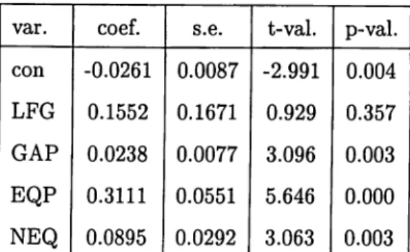
The regression is carried out by using Ordinary Least Squares method. The results obtained from the OLS regression are given in Table 2. The claim that the equipment share o f investment very crucial is supported by the results o f the regression. Some other points deserve attention. First o f all, the coefficient o f the labor force growth is negative which means as GDP per worker growth is increasing the labor force growth is decreasing. Another point is the significance of the regressors. The t-statistics are not listed in the original article. These statistics reveal that labor force growth and the non-equipment share are not significant. This fact should have been considered by the authors.

(24)

var. coef. s.e. t-val. p-val. con -0.0143 0.0103 -1.391 0.170 LFG -0.0298 0.1984 -0.150 0.881 GAP 0.0203 0.0092 2.208 0.031 EQP 0.2654 0.0653 4.064 0.000 NEQ 0.0624 0.0348 1.791 0.079

Table 2: De Long and Summers data set, OLS, = 0.788, F-val=41.6

var. coef. S.e. t-val. p-val.

con -0.02306 0.00899 -2.56440 0.01315

LFG 0.10040 0.17215 0.58290 0.56238

GAP 0.02230 0.00797 2.78277 0.00741

EQP 0.28279 0.05595 5.05444 0.00010

NEQ 0.09147 0.03038 3.01071 0.00396

Table 3: De Long and Summers data set, RLS, B? = 0.843, F-val=57.9

growth is equipment investment and the other causes o f growth are far below the equipment investment.

1.2.2 RLS and LMS

Same data and the same regression equation are used in some robust regression techniques to understand how much results obtained correct and reliable are. Several robust regression techniques are run the first o f which is the Reweighted Least Squares (RLS) based on LMS. The same table is arranged for this technique also.

The RLS simply assigns some weights to the cases o f regression and then reruns OLS. The weights axe based on the LMS. For this regression weights assigned to the cases turned out to be all one except for two cases belonging to Cameroon and Zambia leading to an

(25)

average weight o f 0.97. It is obvious that the data belonging to these countries were having high standardized LMS residuals. The standardized residuals o f LMS for these two countries are 2.57 and -4.65.

The consequences of delivering 0 weights to only these two countries is apparent over the table for RLS. The impact of eliminating these small number o f data points is high on the regression statistics. The B? statistics has risen from 0.78 to 0.84. The F-statistic is also improved from 41.6 in OLS to 57.9 in RLS. Now each o f the regressors but the labor force growth becomes significant, that is, the constant term and the non-equipment investment alter their significance.

The Least Trimmed Squares will also be applied to the same data as well as the Mini mum Volume Ellipsois method. One basic drawback o f the minimum Ellipsoid Method is about its coverage. The method is applied to the regressors only where the regressand may well be contaminated by outliers. And another prominent drawback o f the method is that it just detects the outlying observations and does nothing about qualifying them ats good or bad leverage points and beyond that, the method assigns weights to the cases accord ing to the robust distances calculated. The weights just consider whether the distances exceed the corresponding critical values. Indeed, some cases exceeding these critical values may be very precious good outliers that should never be eliminated by means o f assigning zero weights.

1.2.3 Least Trimmed Squares

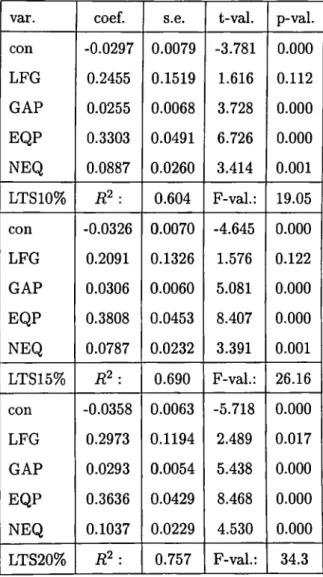
Yet another prominent robust regression technique applied is the Least Trimmed Squares. A Gauss program is written to perform this technique. One important question about the application of the technique is to decide which percentage of the data to trim. Indeed, a parameter is assigned to this percentage in the program. Although so many percentages are tried several o f them are chosen to be reported. Tables 4, and 5 are arranged to display the summary statistics for the LTS where the trimmed percentages begin from 5 percent and goes until 20 percent with equal increments in percentage.

Table 4 suggests that all the regressors but the labor force growth are significant, and the t-statistic for this variable is not as small as the one obtained by OLS. There are some

(26)

Table 4: De Long and Summers data set, LTS, 5 % trim, = 0.518, F-val=14.2

improvements for the significance of all of the regressors. The coefficient for the labor force growth again turns out to be positive.

The trimmed percentage is increased to 10, 15, and 20 percents to note the additional effects of eliminating some more of the data provided that the objective o f the LTS is satisfied.

When the trimmed percentage insreases, there arises a trade-off in between the data lost by being trimmed and the sum of squares of OLS residuals o f the remaining data. Here by incresing the trimmed data percentage from 5 % to 10 % some more cases are lost and there is some more improvement for the and the F-statistics of regression. Some more significance for all of the regressors is achieved as well.

One important result of applying the the LTS algorithm is that we are now able to see the labor force growth among the significant regressors. We were not able to observe this as a consequence of the robust regression techniques we have been trying so far. One can comment on the sign of this regressor depending upon which portion of the business cycle and the marginal productivity of labor the economy is.

1.2.4 Minimum Volume Ellipsoid Method on Growth Data

The last technique to be discussed about is the Minimum Volume Ellipsoid Technique. The software using the technique is fed by the regressors of a data set and then determines the cases to be included and excluded. One important point that deserves attention is that

(27)

var. coef. s.e. t-val. P“val. con -0.0297 0.0079 -3.781 0.000 LFG 0.2455 0.1519 1.616 0.112 GAP 0.0255 0.0068 3.728 0.000 EQP 0.3303 0.0491 6.726 0.000 NEQ 0.0887 0.0260 3.414 0.001 LTS10% B? : 0.604 F-val.: 19.05 con -0.0326 0.0070 -4.645 0.000 LFG 0.2091 0.1326 1.576 0.122 GAP 0.0306 0.0060 5.081 0.000 EQP 0.3808 0.0453 8.407 0.000 NEQ 0.0787 0.0232 3.391 0.001 LTS15% B? : 0.690 F-val.: 26.16 con -0.0358 0.0063 -5.718 0.000 LFG 0.2973 0.1194 2.489 0.017 GAP 0.0293 0.0054 5.438 0.000 EQP 0.3636 0.0429 8.468 0.000 NEQ 0.1037 0.0229 4.530 0.000 LTS20% B? : 0.757 F-val.: 34.3

(28)

the points excluded outside of the ellipsoid may be good or bad leverage points and if the good leverage points are let out, this is a very big loss for the success of the regression.

The software used may try all possible combinations to fix the minimum volume ellip soid or it may select a huge number of combinations. The first one is complete enumeration and results in the best possible performance o f the minimum volume of the ellipsoid, but this requires so much computation time and a powerful computer. On the other hand, the compensation o f the huge number of combinations is at its saving for computation time.

1.3 Detection of G ood and Bad Outliers

G ood leverage points are very precious since they manipulate the regression line towards where it has to, but bad ones are at least as bad to compensate the advantages of the good leverage points. This fact makes the detection of the characteristics o f the data points extremely important. Two main statistics play crucial roles in analyzing these points. The main purpose of detecting the outliers is not to eliminate them. Some RRTs eliminate some of them and some of them delete all o f the outliers regardless of whether they are useful or harmful for the regression.

The two criteria we will follow heavily depends on the robust distances and the stan dardized residuals. The standardized residuals are LMS residuals divided by their standard errors. Since these are supposed to follow the Gaussian Distribution they will hardly be out of the [-2.5,2.5] tolerance band. So we suspect the cases that are outside this band. The second criterion is the robust distances of the cases. Each robust distance should be less than the x l where k is the number of regressors the and percentages may replace (.) depending on the sensitivity of the researcher. If the robust distance exceeds this critical value and the standardized residual is out of the band then the case is marked as a bad leverage point. But if it stays in the tolerance band while the critical value is exceeded then that particular point proves to be a good leverage point. Now we are going to analyze the data sets of the examples with the above method.

The MVE subroutine prepared by Rousseeuw and Leroy, simply checks for the robust distances calculated only and then assigns a weight of 0 or 1 depending on the size o f the robust distance. But this approach suffers from not taking the regressand into account, since the program does not even require the input o f the regressand.

(29)

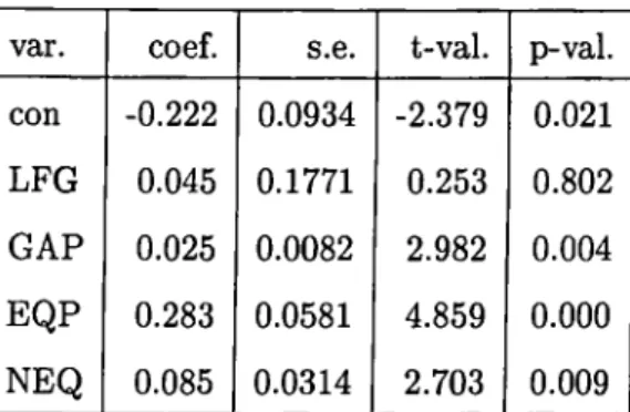
var. coef. s.e. t-val. p-val. con -0.222 0.0934 -2.379 0.021 LFG 0.045 0.1771 0.253 0.802 GAP 0.025 0.0082 2.982 0.004 EQP 0.283 0.0581 4.859 0.000 NEQ 0.085 0.0314 2.703 0.009

Table 6: Regression statistics for De Long and Summers data which considers both robust distances and the standardized residuals, is 0.84 and F-val is 55.8

Finally, a new method that checks for both the standardized LMS residual and the robust distance at the same time is applied to the data. Only one o f the 13 points removed by MVE subroutine is qualified as a bas leverage point and is removed. The procedure expalined above is applied and the only such country to be removed is found to be Zambia. The results of regression when only this country removed is displayed in Table 6. Notice that there arises some alterations in the significance o f the constant term and the non-equipment investment term, the t-values improve from -1.39 to -2.38 for the constant and from 1.79 to 2.70 for the non-equipment term. GAP is also rescued from being borderline significant (t-value is 2.21) to significant (now t-value is 2.98) by using the new method instead of OLS.

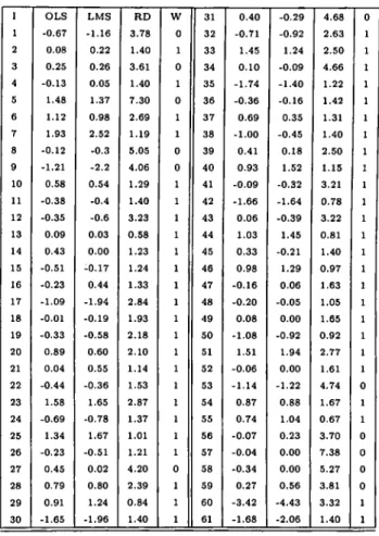
Table 7 lists the standardized residuals by OLS and LMS, and also the robust distances of the MINVOL. Note that there are some differences between the OLS and the LMS standardized residuals.

1.4 G ray’s D ata Set on Aircrafts

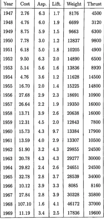
Gray [31] had made a regression to figure out the cost o f building the airctafts from 1947 to 1969. The response variable is the cost whereas the regressors are the weight o f the plane, maximal thrust, lift-to-drug ratio and the aspect ratio. The data set contains 23 years’ data, and no constant is included as a regressor. The same procedure is followed.

(30)

I OLS LMS RD W 31 0.40 -0.29 4.68 0 1 -0.67 -1.16 3.78 0 32 -0.71 -0.92 2.63 1 2 0.08 0.22 1.40 1 33 1.45 1.24 2.50 1 3 0.25 0.26 3.61 0 34 0.10 -0.09 4.66 1 4 -0.13 0.05 1.40 1 35 -1.74 -1.40 1.22 1 5 1.48 1.37 7.30 0 36 -0.36 -0.16 1.42 1 6 1.12 0.98 2.69 1 37 0.69 0.35 1.31 1 7 1.93 2.52 1.19 1 38 -1.00 -0.45 1.40 1 8 -0.12 -0.3 5.05 0 39 0.41 0.18 2.50 1 9 -1.21 -2.2 4.06 0 40 0.93 1.52 1.15 1 10 0.58 0.54 1.29 1 41 -0.09 -0.32 3.21 1 11 -0.38 -0.4 1.40 1 42 -1.66 -1.64 0.78 1 12 -0.35 -0.6 3.23 1 43 0.06 -0.39 3.22 1 13 0.09 0.03 0.58 1 44 1.03 1.45 0.81 1 14 0.43 0.00 1.23 1 45 0.33 -0.21 1.40 1 15 -0.51 -0.17 1.24 1 46 0.98 1,29 0.97 1 16 -0.23 0.44 1.33 1 47 -0.16 0.06 1.63 1 17 -1.09 -1.94 2.84 1 48 -0.20 -0.05 1.05 1 18 -0.01 -0.19 1.93 1 49 0.08 0.00 1.65 1 19 -0.33 -0.58 2.18 1 50 -1.08 -0.92 0.92 1 20 0.89 0.60 2.10 1 51 1.51 1.94 2.77 1 21 0.04 0.55 1.14 1 52 -0.06 0.00 1.61 1 22 -0.44 -0.36 1.53 1 53 -1.14 -1.22 4.74 0 23 1.58 1.65 2.87 1 54 0.87 0.88 1.67 1 24 -0.69 -0.78 1.37 1 55 0.74 1.04 0.67 1 25 1.34 1.67 1.01 1 56 -0.07 0.23 3.70 0 26 -0.23 -0.51 1.21 1 57 -0.04 0.00 7.38 0 27 0.45 0.02 4.20 0 58 -0.34 0.00 5.27 0 28 0.79 0.80 2.39 1 59 0.27 0.56 3.81 0 29 0.91 1.24 0.84 1 60 -3.42 -4.43 3.32 1 30 -1.65 -1.96 1.40 1 61 -1.68 -2.06 1.40 1

Table 7: Minimum Volume Ellipsoid, standardized residuals by OLS and LMS, and weights assigned by the MVE subroutine

(31)

We first run OLS and then we will keep on applying the RRTs starting by RLS, ans LTS. We will finalize this section also by the joint consideration o f the robust distances and the standardized LMS residuals. Data are provided in Table 8.

The results of the OLS regression are given in the following Table 9. The coefficient o f determination is very high and this seems to be a good way of explaining the cost in terms o f the regressors. All the regressors prove to be ¡significant, and the F-statistics for regression is so high to claim that all coefficients of the regression are far from being equal to 0 simultaneously.

There may be some outliers that cannot be detected by the OLS. The residuals over scale with respect to the OLS are searched and it is detected that there are no outliers. That is, all the standardized residuals reside in the band covered by 2.5 standard deviations around 0. Table 10 is prepared to display the standardized residuals by OLS and LMS for the current data. Note that all OLS standardized residuals stay in the [-2.5,2.5] tolerance band, leading to the idea that the data contains no outliers. According to the LMS standardized residuals there are three cases which are not covered by the band for 1960, 1962, and 1968. OLS is unaware of this and does not consider these cases as outliers. All cases are in the band as long as OLS regression is used.

1.4.1 LMS and RLS Based on LMS

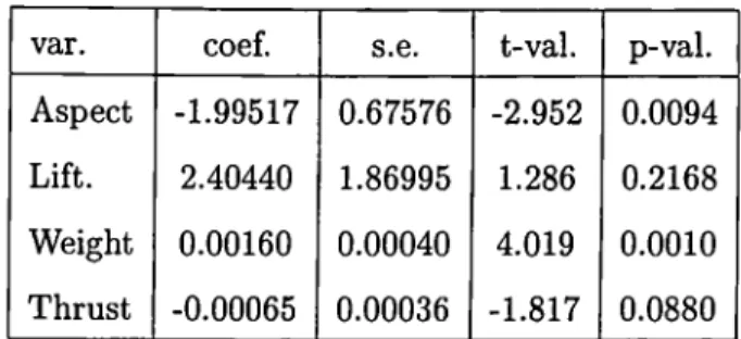
Note that the t-values of the reweighted least squares show that some o f the^regressors proved to be significant according to the LS now loose their significance. There are some substantial changes of the regression statistics compared to the LS regression. The main difference is from the detection of the leverage points. Although some improvement is seen in the coefficient o f determination, the F-statistics for the regression is subject to some smaller values. The coefficients are having substantial changes according to the comparison of the two Tables 9 and 11.

(32)

Year Cost Asp. Lift. Weight Thrust 1947 2.76 6.3 1.7 8176 4500 1948 4.76 6.0 1.9 6699 3120 1949 8.75 5.9 1.5 9663 6300 1950 7.78 3.0 1.2 12837 9800 1951 6.18 5.0 1.8 10205 4900 1952 9.50 6.3 2.0 14890 6500 1953 5.14 5.6 1.6 13836 8920 1954 4.76 3.6 1.2 11628 14500 1955 16.70 2.0 1.4 15225 14800 1956 27.68 2.9 2.3 18691 10900 1957 26.64 2.2 1.9 19350 16000 1958 13.71 3.9 2.6 20638 16000 1959 12.31 4.5 2.0 12843 7800 1960 15.73 4.3 9.7 13384 17900 1961 13.59 4.0 2.9 13307 10500 1962 51.90 3.2 4.3 29855 24500 1963 20.78 4.3 4.3 29277 30000 1964 29.82 2.4 2.6 24651 24500 1965 32.78 2.8 3.7 28539 34000 1966 10.12 3.9 3.3 8085 8160 1967 27.84 2.8 3.9 30328 35800 1968 107.10 1.6 4.1 46172 37000 1969 11.19 3.4 2.5 17836 19600

(33)

var. coef. s.e. t-val. p-val.

Asp. -4.442 0.7780 -5.710 0.00002

Lift 2.482 1.1595 2.140 0.04552

Weight 0.003 0.0005 7.666 0.00000

Thrust -0.002 0.0005 -4.119 0.00058

Table 9: Gray’s Aircraft Data, OLS, = 0.937, F-val=70.97

Year OLS LMS 1958 -1.81 -0.44 1947 0.88 0.00 1959 -0.18 0.41 1948 1.19 0.25 1960 0.01 -2.94 1949 1.27 0.94 1961 -0.11 0.14 1950 -0.82 0.00 1962 0.13 3.85 1951 -0.19 -0.17 1963 -1.50 -0.30 1952 -0.72 -0.11 1964 -0.30 2.03 1953 -0.49 -0.29 1965 0.61 2.26 1954 0.78 0.41 1966 0.92 0.00 1955 -0.13 1.20 1967 -0.37 1.18 1956 -0.97 1.60 1968 2.21 11.04 1957 -0.40 1.94 1969 -0.31 0.00

(34)

Aspect -1.99517 0.67576 -2.952 0.0094

Lift. 2.40440 1.86995 1.286 0.2168

Weight 0.00160 0.00040 4.019 0.0010

Thrust -0.00065 0.00036 -1.817 0.0880

Table 11: Gray’s Aircraft Data, RLS, = 0.942, F-val=64.94

var. coef. S .e . t-val. p-val.

Aspect -2.61821 0.64751 -4.04353 0.00076

Lift. 1.90141 0.79402 2.39467 0.02773

Weight 0.00223 0.00040 5.63467 0.00002

Thrust -0.00106 0.00038 -2.82496 0.01122

Table 12: Gray’s Aircraft Data, LTS 5 percent trim, ií^ = 0.938, F-val=67.98

1.4.2 T h e LTS on G ra y ’s A ircra ft D a ta

First around 5 percent of the data are eliminated and the OLS regression is run with the remaining data. The coefficient o f determination and the F-statistics are close to the ones obtained by OLS, but there are some crucial changes in the coefficients. See Table 12.

When the trimmed percentage increases to 10, both statistics for regression say that this is a more successful regression than the OLS. Indeed, one needs a bencmark to show that the robust regression technique is doing better than OLS and the only two such criteria that we are using are the coefficient o f determination, R? and the F-statistics both of which reveal that now, the LTS is doing better than OLS when some of the cases are eliminated.

The improvement still continues when 20 percent of the data are removed. Note that the statistics belonging to the robust regression techniques are close to each other and

(35)

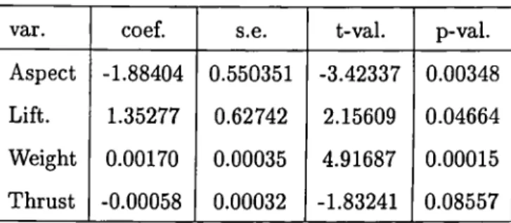
var. coef. s,e. t-val. p-val.

Aspect -1.88404 0.550351 -3.42337 0.00348

Lift. 1.35277 0.62742 2.15609 0.04664

Weight 0.00170 0.00035 4.91687 0.00015

Thrust -0.00058 0.00032 -1.83241 0.08557

Table 13: Gray’s Aircraft Data, LTS 10 percent trim, = 0.951, F-val=77.41

Aspect -1.96283 0.45502 -4.31377 0.00084

Lift. 1.32201 0.50754 2.60476 0.02181

Weight 0.00199 0.00029 6.84605 0.00001

Thrust -0.00081 0.00026 -3.05932 0.00913

Table 14: Gray’s Aircraft Data, LTS 20 percent trim, = 0.973, F-val=118.22

substantially different than the ones by OLS.

1.4.3 Minimum Volume Ellipsoid Method Applied

The subroutine is run to obtain the Minimum Volume Ellipsoid and thereby the outlying cases. The subroutine itself assigns zero weights to two cases but these may be good or bad outliers. To detect whether they are harmful or useful to the appropriateness o f the regression, the robust distances are considered over the standardized residuals. The band for the standardized residuals was already determined as [-2.5,2.5] and the 0.975 percent critical value for the distribution is 11.14. So the robust distance calculated must be more than 3.34 and the standardized LMS residual should be less than -2.5 or higher than 2.5 for the point to be regarded as a bad leverage point. These, and may be the ones near the boundary, must be eliminated from the data set. Although 1960, 1966, and 1968 have their robust distances greater than 3.34, 1960, and 1968 have their standardized residuals

(36)

Aspect -2.921 0.688 -4.248 0.001

Lift. 4.190 2.060 2.034 0.058

Weight 0.002 0.000 4.602 0.000

Thrust -0.001 0.000 -2.917 0.010

Table 15: Gray’s Aircraft Data, Outliers removed using standardized residuals and robust distances together, = 0.941, F-val=67.96

outside the tolerance band. So they are eliminated. Then OLS is run over the remaining data and the results in Table 15 are obtained.

Note that there is a slight improvement in the fit o f the regression line according to the coefficient o f determination, and the coefficients are subject to changes.

1.5 Augm ented Solow M odel

Nonneman and Vanhoudt [72] introduces human capital to the Mankiw, Römer, and Weil’s 1992 study [60] on augmented Solow model. The augmented Solow Model suggests

ln{YtlYo) = /3o + ßiln{YQ) + ß2ln{Sk) + ßzln{N) (15) where Y is real GDP per capita of working age, Sk is average annual ratio o f domestic investment to real GDP, and N is annual population growth,n, plus 5 percent.

Nonneman and Vanhoudt uses the data in Table 16 all throughout their paper. Some times they are changing the regression equation and sometimes they are playing with the regressors included but the data set does not change. Their main objective is to apply the augmented Solow model introduced by Mankiw, Römer and Weil to the OECD countries in a better way.

(37)

Canada USA Japan Austria Belgium Denmark Finland France Germany Greece Ireland Italy Netherlands Norway Portugal Spain Sweden Switzerland Turkey UK Australia New Zealand 1 1 2 3 4 5 6 7 8 9 10 11 12 13 14 15 16 17 18 19

20

21

22

^85 23060 25014 17669 16646 16876 19406 17776 18546 17969 9492 12054 16055 16937 22107 7925 11876 20826 22428 51500 17034 20617 17319 ^60 12361 16364 4648 7827 8609 10515 8630 9650 9819 3164 5454 7086 10008 8977 2965 4916 11364 14532 2884 10004 12824 13569 _ A _ 0.2542 0.2397 0.3658 0.2828 0.2645 0.2915 0.3852 0.2972 0.3095 0.2885 0.2877 0.3139 0.2789 0.3494 0.2608 0.2817 0.2636 0.3142 0.2323 0.2067 0.3128 0.2680 Sh 0.106 0.119 0.109 0.080 0.093 0.107 0.115 0.089 0.084 0.079 0.114 0.071 0.107 0.010 0.058 0.080 0.079 0.048 0.055 0.089 0.098 0.119 gr 0.0125 0.0255 0.0240 0.0110 0.0140 0.0110 0.0120 0.0205 0.0245 0.0020 0.0080 0.0095 0.0205 0.0145 0.0035 0.0045 0.0225 0.0230 0.0020 0.0225 0.0105 0.0095 n 0.0197 0.0154 0.0124 0.0036 0.0045 0.0058 0.0076 0.0099 0.0050 0.0070 0.0105 0.0064 0.0138 0.0068 0.0060 0.0090 0.0031 0.0084 0.0271 0.0033 0.0200 0.0170

(38)

Const. 2.9759 1.0205 2.913 0.009

ln{Yo) -0.3429 0.0565 -6.070 0.000

ln{Sk) 0.6501 0.2020 3.218 0.005

ln{N) -0.5730 0.2904 -1.973 0.064

Table 17: Augmented Solow Model, OLS, B? = 0.746, F-val=17.7

1.5.1 O LS an d L M S

If there is no robust regression technique applied, the OLS regression gives the coefficients and regression results tabled in 17

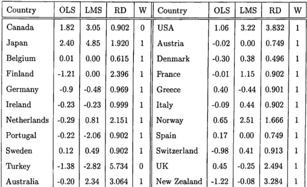
Table 18 orders the OLS and the LMS standardized residuals, as well as the weights assigned by the MVE method. These weights are taken into consideration and the cases penalized by zero weights are eliminated from the data set, and OLS is run over the remaining ones to see the results obtained by the MVE algorithm. These weights by the MVE algorithm are assigned according to the robust distances (RD) of the corresponding cases. Note that cases 1 and 19 are assigned 0 weights and these are the cases with the highest robust distances. Indeed, the MVE just checks whether the RDs are exceeding the critical values or not, and the cases exceeding the critical values are addressed as

the bad leverage points and assigned zero weights. It is no coincidence that these are the cases with maximum robust distances.

RLS based on LMS leads to the coefficient of determination equal to 0.971 which is higher than 0.746 of OLS, there is some improvement in terms of the F-statistic o f regression also. There are some considerable changes in the coefficients of the regressors as well. One o f the main differences between the RLS and the OLS is the significance o f population growth in the regression equation. The neoclassical theory of growth claims that the growth rate o f population is effective in determining the GDP growth and so does the enogeneous growth theory in the short run, so the result obtained by RLS is more plausible. The cases deleted by the LMS algorithm are 1, 2, 3, 14, and 19. See Table 19.

(39)

Country Canada Japan Belgium Finland Germany Ireland Netherlands Portugal Sweden Turkey Australia OLS 1.82 2.40 0.01 -1.21 -0.9 -0.23 -0.29 -0.22 0.12 -1.38 -0.20 LMS 3.05 4.85 0.00

0.00

-0.48 -0.23 0.81 -2.06 0.49 -2.82 2.34 RD 0.902 1.920 0.615 2.396 0.969 0.999 2.151 0.902 0.902 5.734 3.064 W

0

1 1 1 1 1 1 1 1

0

1 Country USA Austria Denmark Prance Greece Italy Norway Spain Switzerland UK New Zealand OLS 1.06 -0.02 -0.30 -0.01 0.40 -0.09 0.65 0.17 -0.98 0.45 -1.22 LMS 3.22 0.00 0.38 1.15 -0.44 0.44 2.51

0.00

0.41 -0.25 -0.08 RD 3.832 0.749 0.496 0.902 0.901 0.902 1.666 0.749 0.913 2.494 3.284 W 1 1 1 1 1 1 1 1 1 1 1

Table 18: Augmented Solow Model, OLS and LMS standardized residuals, and weights assigned by MVE

Const. 2.4949 0.5193 4.805 0.001

ln{Yo) -0.4437 0.0260 -17.054 0.000

ln{Sk) 0.3208 0.0807 3.975 0.002

ln{N) -0.9037 0.1575 -5.737 0.000

(40)

The LTS subroutine is run over the same data set. 5, 10, 15, and 20 percent trim’s regeression results are tabled in the same fashion. The only country deleted for 5 percent trim is Canada, 10 percent trim only adds Japan, and 15 percent trim adds USA to the deleted countries. Finally 20 percent trim deleted Australia additionally. Table 20 lists all results for the LTS. Notice that the coefficient o f variation is increasing as more data points are deleted. The more data points eliminated according the LTS objective, the more successful the fit is, finally 20 percent fit leads to much better results than OLS.

The Minimum Volume Ellipsoid tried all combinations possible and found out that Canada, and Turkey should be eliminated to have a better regression. The results obtained here are similar to the ones obtained by other robust regression techniques. The most stimulating drawback of MVE seems to be its rejecting the significance o f population growth. Refer to Table 21 for regression results.

The robust distances o f MVE and the standardized LMS residuals are simultaneously considered to identify the bad leverage point. The only such point is from Turkey. Re moving Turkey’s data gives the tabled results in Table 22. Notice that the population growth turned out to be insignificant again.

I . 6 Benderly and Zwick’s Return D ata

J. Benderly, and B. Zwick’s data set from A E R [4] aims to explain the return on common stocks by output growth and inflation over 1954-1981 period. Indeed, they would like to make some contribution to the original article by Fama [26] on the significance o f inflation to determine the real stock returns. The regression equation concentrated on is

Rt = /3o + PiGt + P2h

(16)

where R is the real stock return, G is the output growth in percentage, and I stands for inflation in percentage again. Here R is measured using Ibbotson-Sinquefeld data base, G is measured by real GDP, and P is measured by the deflator for personal consumption expenditures.

(41)

var. coef. s.e. t-val. p-val. Const. 1.8730 0.8506 2.202 0.042 ln{Yo) -0.3010 0.0454 -6.632 0.000 ln{Sk) 0.3955 0.1721 2.298 0.035 ln(N) -0.7108 0.2287 -3.108 0.006 LTS5 : 0.780 F-val.: 20.1 Const. 1.5979 0.6933 2.305 0.035 IniXo) -0.3255 0.0375 -8.679 0.000 ln{Sk) 0.4568 0.1105 3.250 0.005 ln{N) -0.9093 0.1953 -4.656 0.000 LTSIO : 0.864 F-val: 34.0 Const. 1.7573 0.5951 2.953 0.010 ln{Yo) -0.3624 0.0349 -10.370 0.000 ln{Sk) 0.5670 0.1271 4.462 0.000 ln{N) -1.0154 0.1715 -5.919 0.000 LTS15 R? : 0.900 F-val.: 44.9 Const. 1.4047 0.5764 2.437 0.029 ln{Yo) -0.3822 0.0337 -11.338 0.000 ln{Sk) 0.5337 0.1180 4.520 0.000 ln{N) -1.1850 0.1804 -6.571 0.000 LTS20 : 0.916 F-val.: 51.1

(42)