Memory-efficient multilevel physical optics algorithm for fast computation of scattering from three-dimensional complex targets

Memory-Efficient Multilevel Physical Optics

Algorithm for Fast Computation of Scattering From

Three-Dimensional Complex Targets

Alp Manyas

1,2

_{and Levent G¨urel}

1,2

1_{Department of Electrical and Electronics Engineering} 2_{Computational Electromagnetics Research Center (BiLCEM)}

Bilkent University, TR-06800, Bilkent, Ankara, Turkey {alp, lgurel}@ee.bilkent.edu.tr

Abstract— Multilevel physical optics (MLPO) algorithm

pro-vides a speed-up for computing the physical-optics integral over complex bodies for a range of aspect angles and frequencies. On the other hand, when computation of the RCS pattern as a function of θ, φ, and frequency is desired, the O N3

memory complexity of the algorithm may prevent the solution of electrically large problems. In this paper, we propose an improved version of the MLPO algorithm, for which the memory complexity is reduced to O N2_{log N . The algorithm is based}

on the aggregation of only some portion of the scattering patterns at each aggregation step. This way, memory growth in each step is prevented, and a significant amount of saving is achieved.

I. INTRODUCTION

For the computation of electromagnetic scattering from electrically large targets, physical-optics (PO) technique can provide very fast solutions. On the other hand, in real-life radar applications, where the computation of the scattering pattern over a range of frequencies and/or angles with sufficient number of samples is desired, further acceleration may be needed. Multilevel physical optics (MLPO) algorithm [1], [2] can be used for such applications, so that a remarkable speed-up can be achieved by evaluating the PO integral in a multilevel fashion. One of the drawbacks of this algorithm is its rapidly growing memory requirement for three-dimensional (3-D) applications. In this paper, a memory-efficient multidi-mensional MLPO algorithm, with which the scattering pattern of a 3-D target can be evaluated as function of elevation angle (θ), azimuth angle (φ), and frequency with a lower memory complexity, is presented. In this algorithm, memory complexity of O¡N3¢_{is reduced to O}¡_N2_{log N}¢_.

II. MLPO ALGORITHM

A. Computation Time

When computing the PO scattering pattern with sufficient number of samples as a function of θ, φ, and frequency, sampling rate in each dimension should be proportional to the electrical size of the target. Let R be the smallest radius of a sphere that can contain the target and N = kR, where k is the wavenumber. Then, the required number of samples in

θ, φ, and frequency are O (N ) each and the total number of

required samples is O¡N3¢_{. If the target surface is modeled}

with a triangular mesh, there will be O¡N2¢ _{triangles as}

the number of triangles will be proportional to the surface area. Hence, the computational complexity of evaluating PO integral analytically [3] on the triangular mesh for each θ, φ, and frequency turns out to be O¡N5¢_.

Since the origin of the each subdomain will be different from the global origin, subdomain patterns will oscillate at higher rates because of the phase shift. Therefore, prior to interpolation, subdomain patterns should be shifted to the origin and restored after interpolation. In this scheme, PO operator Ψ that computes the scattering pattern of any arbitrary surface S can be written as

ΨS =XQ

q=1E [¯rq] I NθNφNf

¯

NθN¯φN¯fO [¯rq] Ψ ¯Sq. (1)

Here, ¯rq is the center of the smallest sphere that can include

the qth subdomain. O [¯rq] is the operator that shifts the origin

of the qth subdomain to the global origin in order to remove the phase oscillations. The INθNφNf

¯

NθN¯φN¯f matrix is the interpolation

matrix that increases the number of samples from ¯Nθ× ¯Nφ×

¯

Nf points to Nθ× Nφ× Nf points, and E [¯rq] is the operator

that shifts the origin of the qth subdomain back to its location after the interpolation.

In the MLPO algorithm, each subdomain is recursively subdivided into smaller subdomains and the scattering patterns of these subdomains are also calculated via MLPO. When the subdomain size is in the order of λ (wavelength), the subdivision process can be stopped and the scattering patterns of the lowest-level subdomains can be evaluated with the PO integral.

As the electrical size of the bottom-level subdomains will be bounded, the required number of θ, φ, and frequency samples will be fixed for each subdomain at this level. There will be O¡N2¢ _{filled subdomains at this level and therefore}

calculating the PO patterns of all subdomains analytically at this level will require O¡N2¢_{operations. At each aggregation}

step, local interpolations transforming the scattering patterns form a coarse grid of θ, φ, and frequency to a finer grid will require O¡N3¢_{operations. As there will be O (log N ) levels,}

Therefore, the overall complexity of the MLPO algorithm is

O¡N2¢_{+ O}¡_N3_{log N}¢_{= O}¡_N3_{log N}¢_{. This complexity is}

far less than the O¡N5¢ _{complexity of the conventional PO}

integration.

B. Memory Requirement

The MLPO algorithm requires O¡N3¢_{memory to store the}

radiation patterns for all three dimensions when aggregating from lower levels to the upper levels, since the sampling rates in each of the three dimensions will be doubled. Therefore, the required memory for each cluster will grow by a factor of 8. Since PO current is only on the surface of the target, we can assume that the number of filled clusters is O¡N2¢

at the bottom level. We can also assume that the number of filled clusters is reduced by a factor of 4 at each higher level. Therefore, the memory required at each aggregation step will increase by a factor of 8/4 = 2. Hence, at the uppermost level, the memory requirement will be O¡N2₂log N¢_{, which}

is O¡N3¢_{. As will be shown in Section IV, this memory}

requirement may prevent the solution of larger problems using the MLPO algorithm. In the next section, we present a memory-efficient implementation that reduces the memory complexity from O¡N3¢_{to O}¡_N2_{log N}¢_.

III. MEMORY-EFFICIENTMLPO ALGORITHM

The proposed memory-efficient implementation of the MLPO algorithm is based on the idea that the patterns of the clusters need not be stored for the entire range of θ, φ, or frequency values at the same time. By careful implementation, the θ, φ, or frequency ranges can be divided into smaller ranges so that interpolations and aggregations can be performed on those smaller ranges.

For instance, when aggregating the bottom level to the upper level, θ can be sampled in the£0,π

2

¤

range instead of [0, π]. This way, the memory required for each cluster will grow by a factor of 4 instead of 8. In the next level, the number of clusters will be reduced by a factor of 4, and the total required memory will be constant. Then, θ can be sampled in the£0,π

4

¤ range instead of £0,π

2

¤

at the next level, and this procedure can be applied till the uppermost level is reached. This scheme is illustrated in Fig. 1.

If L is the number of levels, after the aggregations are performed, 1±2L−1 _{portion of whole scattering pattern will}

be available at the Lth level. This portion can be output to a file and the remaining portion can be obtained by aggregating the second half of the pattern available at the (L − 1)st level to the Lth level. Then, the 3rd portion of the pattern will be required. This portion will not be available at the (L − 1)st level. Therefore, the pattern available at the (L − 2)nd level should be aggregated to the (L − 1)st level. Then, the 3rd portion of the whole scattering pattern at the Lth level can be obtained by aggregation from the (L − 1)st level. In this scheme, after 2L−1 _{passes, the whole scattering pattern will}

be obtained. As an example, aggregations of pattern portions for a 6-level problem is depicted in Fig. 2

. . .

[

0 : :

]

samples N_θ θ∈ ∆θ π 0 : : 2 2 samples N_θ θ π θ_{∈ } ∆ _   0 : : 4 4 samples N θ θ π θ_{∈ } ∆ _   . . .

Fig. 1. Aggregation steps in the proposed memory-efficient algorithm. Note that θ ∈ [0 : ∆θ : π] means that the pattern at that level is sampled from 0 to π with an increment of ∆θ

The following pseudo-code describes partial aggregation of the clusters at each pass:

{n is an array of size L − 1, indicating which half of the

available pattern portion should be aggregated at each pass.}

{In the first pass, first halves of the available pattern portions

should be aggregated.}

n(1 : L) ← 1

for t = 1 to 2L−1 _do

for l = 1 to L − 1 do {all levels 1 to L − 1}

m ← L − l + 1

if mod¡t, 2m−2¢_{= 1 or m= 2 then}

for all cli ∈ lth_{level do {all clusters in lth level}} {Aggregate the n(l)th half of the cluster.} aggregate cluster(cli, n(l)) end for if n(l) = 1 then n(l) ← 2 else n(l) ← 1 end if end if end for

{Write the available portion of the whole targets

scatter-ing pattern.}

writeT oF ile

end for

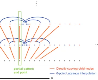
It should be noted that higher-order interpolation schemes may be desired in order to prevent interpolation error in aggregations [4]. In this case, additional sample points at the end points of the partial patterns should be included at the interpolations as illustrated in Fig. 3.

For the end points corresponding to θ = 0 or θ = π, the samples corresponding to neighboring nodes on the unit sphere can be used since (0 − α, φ) = (α, φ + π) and (π + α, φ) = (π − α, φ + π) on a unit sphere.

Dividing the ranges of other dimensions will reduce the required memory at each aggregation step but will not

signif-passes le v e ls

. . .

output to file output to file output to file output to file output to file output to file output to file output to file output to file 1 0, 32       2 0, 32       4 0, 32       8 0, 32       16 0, 32       32 0, 32       2 0, 32       2 0, 32       4 0, 32       8 0, 32       16 0, 32       32 0, 32       2 3 , 32 32       2 4 , 32 32       4 0, 32       8 0, 32       16 0, 32       32 0, 32       3 4 , 32 32       2 4 , 32 32       4 0, 32       8 0, 32       16 0, 32       32 0, 32       4 5 , 32 32       4 6 , 32 32       4 8 , 32 32       8 0, 32       16 0, 32       32 0, 32       5 6 , 32 32       4 6 , 32 32       4 8 , 32 32       8 0, 32       16 0, 32       32 0, 32       6 7 , 32 32       6 8 , 32 32       4 8 , 32 32       8 0, 32       16 0, 32       32 0, 32       7 8 , 32 32       6 8 , 32 32       4 8 , 32 32       8 0, 32       16 0, 32       32 0, 32       8 9 , 32 32       8 10 , 32 32       8 12 , 32 32       8 16 , 32 32       16 0, 32       32 0, 32       9 10 , 32 32       10 11 , 32 32       12 13 , 32 32       13 14 , 32 32       14 15 , 32 32       11 12 , 32 32       8 10 , 32 32       10 12 , 32 32       10 12 , 32 32       12 14 , 32 32       12 14 , 32 32       14 16 , 32 32       8 12 , 32 32       8 12 , 32 32       8 12 , 32 32       12 16 , 32 32       12 16 , 32 32       12 16 , 32 32       8 16 , 32 32       8 16 , 32 32       8 16 , 32 32       8 16 , 32 32       8 16 , 32 32       8 16 , 32 32       16 0, 32       16 0, 32       16 0, 32       16 0, 32       16 0, 32       16 0, 32       32 0, 32       32 0, 32       32 0, 32       32 0, 32       32 0, 32       32 0, 32       output to file output to file output to file output to file output to file output to file

Fig. 2. Aggregations of pattern portions for a 6-level problem. Aggregations are shown as blue arrows and outputs to files are shown as red arrows.

x o x o x o x o x o o x o x o x x x x x x x x x x x x x x x x x x x – x – x – x – x – x – x – x – x partial pattern end point . . . . . .

Directly copying child nodes

6-point Lagrange interpolation

θ

x

Fig. 3. Interpolating cluster patterns near the end points.

icantly improve the memory efficiency. This is because the patterns of the bottom-level clusters dominate the memory requirement. On the other hand, aggregating the bottom-level clusters directly to the upper level without storing their patterns will reduce the required memory.

IV. NUMERICALRESULTS

To demonstrate the accuracy and efficiency of the MLPO algorithm, backscattering RCS pattern of the scaled Flamme geometry [5] shown in Fig. 4 is computed for all directions on the unit sphere.

RCS values are evaluated for the frequency ranges given in Table I, and CPU times are compared in Figure 7. For the sake of simplicity, first column of Table I is given as N/2π, which is the electrical size of the target in λ.

From the backscattering RCS results shown in Fig. 5, it is

(a) (b) 0.23 m 0.6 m (6λ @ 3GHz) (c) 0. 23 m (d)

Fig. 4. Geometry of the stealth Flamme target: (a) Front view. (b) A uniform mesh example. (c) Rear view. (d) Top view.

TABLE I

GROWTH OF THE NUMBER OF TRIANGLES, θSAMPLES, φSAMPLES,AND

FREQUENCY SAMPLES ASNINCREASES

N/2π (Target Size/λ Number of _N

θ Nφ Nf in Frequency Range) Triangles

[0, 1.5] 628 49 101 17 [0, 3] 1604 97 201 33 [0, 6] 5200 193 401 65 [0, 12] 19288 385 801 129 [0, 24] 75634 769 1601 257 [0, 48] 300020 1537 3201 513

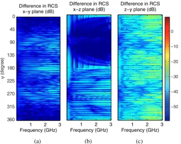
observed that, on the x-y, x-z, and y-z planes and in the 0– 3 GHz frequency range, the MLPO algorithm and direct PO evaluation results are in excellent agreement. Fig. 6 presents the RCS error, 10 log |RCSM LP O− RCSP O|, which is below

1%.

From Table I, it is observed that, as N increases, the number of triangles grows with O¡N2¢ _{for large N . Numbers of θ,}

ψ (degr ee) 0 45 90 135 180 225 270 315 360 Frequency Backscattering RCS x−y plane (dBms) 1 2 3 (a) Frequency Backscattering RCS x−z plane (dBms) 1 2 3 (b) Frequency Backscattering RCS z−y plane (dBms) 1 2 3 (c) −50 −40 −30 −20 −10 0

Fig. 5. Backscattering RCS pattern of the Flamme geometry: (a) x-y, (b) x-z, and (c) z-y planes.

ψ (degr ee) 0 45 90 135 180 225 270 315 360 Frequency (GHz) Difference in RCS x−y plane (dB) 1 2 3 (a) Frequency (GHz) Difference in RCS x−z plane (dB) 1 2 3 (b) Frequency (GHz) Difference in RCS z−y plane (dB) 1 2 3 (c) −50 −40 −30 −20 −10 0

Fig. 6. Absolute error of the MLPO algorithm: (a) x-y, (b) x-z, and (c) z-y planes.

φ, and frequency samples (Nθ, Nφ, and Nf, respectively)

increase with O (N ). Therefore, the total complexity of the direct PO evaluation turns out to be O¡N5¢_{. This can be}

verified from the computation times presented in Fig. 7. Since both axes are in log scale, slopes of the curves indicate the complexity. For instance, log¡N5¢ _{= 5 log (N ) and when}

plotted versus log (N ), the curve is a straight line with slope 5. Similarly, log¡N3_{log (N )}¢ _{= 3 log (N ) + log (log N ) ≈}

3 log (N ) and when plotted versus log (N ), the curve is approximately a straight line with slope 3.

For the 48λ problem presented in Table I and Fig. 7, computing the scattering pattern with the memory-efficient MLPO algorithm takes approximately 53 hours. Computation time of the same problem with the direct PO integration is estimated to be 180,000 hours. Thus, a speed-up of nearly 3000 can be achieved with the MLPO algorithm. On the other

101 102 103 10−2 100 102 104 106 108 1010 N

CPU time (minutes)

CPU times of different PO evaluations Direct evaluation MLPO Memory−efficient MLPO (a) 101 102 103 10−2 100 102 104 106 108 N Memory Requirement (MB)

Memory requirement of the MLPO algorithm MLPO

Memory−efficient MLPO

(b)

Fig. 7. Efficiency of the MLPO algorithm: (a) CPU time. (b) Memory requirement. Dashed curves represent estimated values.

hand, conventional MLPO algorithm would require 388 GB of memory, whereas the memory-efficient MLPO algorithm requires only 5 GB of memory, which is 77 times more efficient.

V. CONCLUSIONS

For 3-D problems, a memory-efficient MLPO algorithm is proposed to evaluate the PO integral, so that the memory complexity of O¡N3¢ _{is reduced to O}¡_N2_{log N}¢_{. The}

backscattering RCS pattern of a stealth geometry is calculated via the proposed algorithm and the results are compared with the direct PO evaluation in order to verify the accuracy and efficiency of the algorithm. For a 48λ problem, it is shown that the MLPO algorithm can achieve a speed-up of more than 3000 at the cost of requiring 388 GB of memory. In addition to achieving a similar speed-up, the memory-efficient MLPO

algorithm can further reduce the memory requirement by a factor of 77, thus enabling the solution of the same problem with 5 GB of memory.

ACKNOWLEDGMENT

This work was supported by the Scientific and Technical Re-search Council of Turkey (TUBITAK) under ReRe-search Grant 105E172, by the Turkish Academy of Sciences in the frame-work of the Young Scientist Award Program (LG/TUBA-GEBIP/2002-1-12), and by contracts from ASELSAN and SSM.

REFERENCES

[1] A. Boag, “A fast physical optics (FPO) algorithm for high frequency scattering,” IEEE Trans. Antennas Propagat., vol. 52, pp. 197–204, Jan. 2004.

[2] A. Boag and E. Michielssen, “Fast physical optics (FPO) algorithm for double-bounce scattering,” IEEE Trans. Antennas Propagat., vol. 52, pp. 205–212, Jan. 2004.

[3] W. B. Gordon, “Far-field approximations to the Kirchhoff-Helmholtz representation of scattered fields,” IEEE Trans. Antennas Propagat., vol. 23, pp. 590–592, July 1975.

[4] A. Manyas and L. G¨urel, “Multilevel PO algorithm for non-uniform triangulations,” European Conference on Antennas and Propagation

(EuCAP 2006), Nice, France, Nov. 2006.

[5] L. G¨urel, H. Ba˘gcı, J. C. Castelli, A. Cheraly, and F. Tardivel, “Validation through comparison: measurement and calculation of the bistatic radar cross section (BRCS) of a stealth target,” Radio Science, vol. 38, no. 3, pp. 12-1–12-10, June 2003.