Generating 3D thumbnails for 3D contents

a thesis

submitted to the department of computer engineering

and the institute of engineering and science

of b˙ilkent university

in partial fulfillment of the requirements

for the degree of

master of science

By

Yeliz Yi˘

git

August, 2010

Asst. Prof. Dr. Tolga C¸ apın(Advisor)

I certify that I have read this thesis and that in my opinion it is fully adequate, in scope and in quality, as a thesis for the degree of Master of Science.

Prof. Dr. B¨ulent ¨Ozg¨u¸c

I certify that I have read this thesis and that in my opinion it is fully adequate, in scope and in quality, as a thesis for the degree of Master of Science.

Asst. Prof. Dr. Tolga Can

Approved for the Institute of Engineering and Science:

Prof. Dr. Levent Onural Director of the Institute

Yeliz Yi˘git

M.S. in Computer Engineering Supervisor: Asst. Prof. Dr. Tolga C¸ apın

August, 2010

Creating effective thumbnails is a challenging task because finding important features and preserving the quality of the content is difficult. Additionally, as the popularity of 3D technologies is increasing, the usage area of 3D contents and the 3D content databases are expanding. However, for these contents, 2D thumbnails are insufficient since the current methods for generating them do not maintain the important and recognizable features of the content and give the idea of the content.

In this thesis, we introduce a new thumbnail format, 3D thumbnail that helps users to understand the content of the 3D graphical scene or 3D video + depth by preserving the recognizable features and qualities.

For creating 3D thumbnails, we developed a framework that generates 3D nails for different 3D contents in order to create meaningful and qualified thumb-nails. Thus, the system selects the best viewpoint in order to capture the scene with a high amount of detail for 3D graphical scenes. On the other hand, this process is different for 3D videos. In this case, by a saliency-depth based ap-proach, we find the important objects on the selected frame of the 3D video and preserve them. Finally, after some steps such as placement, 3D rendering etc., the resulting thumbnails give more glorified information about the content.

Finally, several experiments are presented which show that our proposed 3D thumbnail format is statistically (p <0.05 ) better than 2D thumbnails.

Keywords: 3D thumbnails, 3D contents, best viewpoint selection, viewpoint

en-tropy, saliency, computer graphics.

RES˙IMLER YARATMA

Bilgisayar M¨uhendisli˘gi, Y¨uksek Lisans Tez Y¨oneticisi: Asst. Prof. Dr. Tolga C¸ apın

A˘gustos, 2010

Bir i¸cerik i¸cin anlamlı, etkili k¨u¸c¨uk resimler yaratmak zordur ¸c¨unk¨u bir i¸ceri˘gin ¨

onemli ¨ozelliklerini bulmak ve kalitesini korumak bazı problemleri beraberinde ge-tirmektedir. Buna ek olarak, 3B teknolojilerin pop¨uleritesi arttık¸ca, 3B i¸ceriklerin ve bu i¸ceriklerin veritabanlarının kullanım alanı artmaktadır; ancak bu i¸cerikleri temsil eden 2B k¨u¸c¨uk resimler, bu i¸ceriklerin ¨onemli ¨ozelliklerini ve kalitelerini koruyamadıkları ve kullanıcıya ilk bakı¸sta i¸cerik hakkında bilgi veremedikleri i¸cin yeterli de˘gillerdir.

Bu ¸calı¸smada, yeni bir k¨u¸c¨uk resim formatı sunulmu¸stur, 3B k¨u¸c¨uk resim. Bu format, kullanıcıların 3B grafiksel sahnelerin veya 3B derinli˘gi olan videoların i¸ceriklerini, bu i¸ceriklerin farkedilebilir ¨ozelliklerini ve kalitelerini koruyarak an-lamasını sa˘glamaktadır.

Bu tezde, farklı i¸cerikler i¸cin anlamlı ve kaliteli 3B k¨u¸c¨uk resimler yaratan bir sis-tem geli¸stirilmi¸stir. Bu sissis-tem, farklı i¸cerikler i¸cin farklı ¸sekilde ¸calı¸smaktadır. 3B grafiksel sahneler i¸cin, sahne hakkında en ¸cok bilgiyi i¸ceren bakı¸s a¸cısı se¸cilmektedir. 3B derinli˘gi olan videolar i¸cin ise videonun bir karesi alınarak, ¨

uzerindeki ¨onemli nesneleri bulmak ve onları korumak i¸cin ¸cıkıntı-derinleme ta-banlı bir yakla¸sım izlenmektedir. Daha sonra, nesne yerle¸stirmesi, 3B sahneleme gibi ba¸ska i¸slemler uygulanmaktadır. Sonu¸cta yaratılan k¨u¸c¨uk resimler daha kaliteli ve anla¸sılabilirdir.

Son olarak bu tezde, ¨onerilen 3B k¨u¸c¨uk resim formatının 2B k¨u¸c¨uk resimlerden istatiksel olarak (p <0.05 ) daha ba¸sarılı oldu˘gunu g¨osteren bazı testlere de yer verilmektedir.

Anahtar s¨ozc¨ukler : 3B k¨u¸c¨uk resimler, 3B i¸cerikler, en iyi bakı¸s a¸cısı se¸cimi, bakı¸s

To my family,

Firstly, I would like to express my gratitude to my supervisor Asst. Prof. Dr. Tolga C¸ apın for his support, guidance and encouragement.

I would also like to thank Prof. Dr. B¨ulent ¨Ozg¨u¸c and Asst. Prof. Dr. Tolga Can for serving as members of my thesis committee, accepting my invitation without hesitation and evaluating this thesis.

I want to thank to my beautiful parents, and my lovely sister Yelda, for their support, patience, encouragement and invaluable love through all of my life. They are the meaning of my life. Without their everlasting love and support, this thesis would never be completed.

Furthermore, I am grateful for the support and encouragement of my sunshine, Mehmet Esat Ba¸sol and my best friend and sister, ¨Ozge Dermanlı, who were very understanding and patient while writing my thesis and depressive moments. I am also grateful to all of my friends who filled my life with joy.

Special thanks to my friends for their patience during user experiments. Es-pecially, thanks to S. Fatih ˙I¸sler and Bertan G¨undo˘gdu for their support and help.

Finally, I would like to acknowledge the European Commission’s Seventh Framework Programme project, “All 3D Imaging Phone“ for the financial support of this work.

1 Introduction 1

2 Related Work 5

2.1 Viewpoint Selection Methods . . . 5

2.1.1 Computer Graphics . . . 6

2.1.2 Viewpoint Selection in Other Research Areas . . . 7

2.2 Thumbnail Generation Methods . . . 9

2.3 3D Video Formats . . . 10

2.3.1 Conventional Stereo Video (CSV) . . . 11

2.3.2 Video Plus Depth (V+D) . . . 13

2.3.3 Multiview Video Plus Depth (MVD) . . . 13

2.3.4 Layered Depth Video (LDV) . . . 14

3 Thumbnail Generation System 17 3.1 System Overview . . . 17

3.1.1 Content Analysis . . . 18

3.1.2 Object Ranking . . . 18

3.1.3 Transformation Modeling . . . 19

3.1.4 3D Rendering . . . 20

4 Thumbnail For 3D Graphical Scenes 22 4.1 Overview . . . 22

4.2 Content Analysis . . . 23

4.2.1 Best Viewpoint Selection . . . 23

4.3 Object Ranking . . . 33

4.4 Transformation Modeling . . . 34

4.4.1 Scaling . . . 34

4.4.2 Positioning . . . 36

4.5 Results . . . 39

5 Thumbnail For 3D Videos 40 5.1 Overview . . . 40

5.2 Selected 3D Video Format . . . 41

5.3 Content Analysis . . . 42

5.3.1 Video Frame Selection . . . 42

5.3.2 Image Segmentation . . . 43

5.4 Object Ranking . . . 44

5.5 Transformation Modeling . . . 47

5.5.1 Background Resynthesis . . . 47

5.5.2 Pasting of Visually Significant Objects . . . 48

5.5.3 3D Mesh Generation . . . 48

5.6 Results . . . 49

6 Thumbnail Format and Layouts 51 6.1 Thumbnail Format . . . 51

6.1.1 For 3D Graphical Scenes . . . 51

6.1.2 For 3D Videos + Depth . . . 52

6.2 Layouts . . . 54

7 Experiments and Evaluation Results 56 7.1 2D Thumbnails vs. 3D Thumbnails for 3D Graphical Scenes . . . 56

7.2 2D Thumbnails vs. 3D Thumbnails for 3D Videos + Depth . . . . 59

7.3 3D Meshes vs. Parallax Shading . . . 64

7.4 General Discussion . . . 67

7.4.1 Performance . . . 67

7.4.2 Analysis . . . 69

8 Conclusion and Future Work 71

A.1 Mean-Shift Image Segmentation . . . 81

2.1 Three exploration trajectories followed by the method by Dorme

[15]. . . 6

2.2 A comparison between existing image resizing techniques and au-tomatic image retargeting method[49]. . . 10

2.3 CSV - left and right view. (ballet sequence is used by the courtesy of Interactive Visual Media Group at Microsoft Research.) . . . . 12

2.4 V+D - color video and depth map. (ballet sequence is used by the courtesy of Interactive Visual Media Group at Microsoft Research.) 13 2.5 MVD with 8 views. (ballet sequence is used by the courtesy of Interactive Visual Media Group at Microsoft Research.) . . . 15

2.6 LDV format. (ballet sequence is used by the courtesy of Interactive Visual Media Group at Microsoft Research.) . . . 16

3.1 General 3D thumbnail system. . . 17

3.2 Content analysis. . . 18

3.3 Object ranking. . . 19

3.4 Transformation modeling. . . 20

3.5 3D effects. . . 21

4.1 Shannon’s third requirement[58]. . . 25

4.2 The camera positions that represents viewpoints[58]. . . 28

4.3 Color-coded complex objects. . . 30

4.4 Comparison of viewpoint entropy calculation methods[10]. . . 31

4.5 Results of viewpoint selection by using entropy[59]. (From Pere Pau V´azquez. Reproduced with kind permission of AKA Verlag Heidelberg from the Proceedings of the Vision Modeling and Vi-sualization Conference 2001 ISBN:3-89838-028-9.) . . . 31

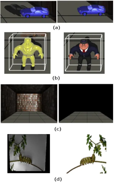
4.6 Figure (a), (b), (c), and (d) show rendered objects from a set of viewpoints. Figure (d) illustrates the best viewpoints. . . 33

4.7 Scaling results. . . 36

4.8 Positioning layout. . . 37

4.9 3D thumbnails. . . 39

5.1 Overview of the 3D thumbnail generation for 3D videos. . . 41

5.2 Saliency-based frame selection: Frame 0, 77, 103 and 211. The most salient one is the frame 103. . . 43

5.3 Mean-shift segmentation with different parameters. (a) Original Image; (b) hs = 7, hr = 6 and M = 800, number of regions: 31, 15, 19; (c) hs = 6, hr = 5 and M = 50, number of regions: 214, 268, 246; (d) hs= 32, hr = 30 and M = 150, number of regions: 1, 7, 6. . . 45

5.4 Graph-based saliency map. a) Original image; b) salient parts of the image (red - most salient); c) resulting saliency map. . . 46

6.1 Thumbnail format for 3D graphical scenes. . . 53

6.2 3D grid layout. . . 54

6.3 2D grid layout. . . 55

6.4 3D grid layout with inclination. . . 55

7.1 2D thumbnail vs. 3D thumbnail for 3D graphical scenes - (based on search time). . . 58

7.2 2D thumbnail vs. 3D thumbnail for 3D graphical scenes - (based on number of clicks performed in order to reach the target thumbnail). 59 7.3 2D thumbnail vs. 3D thumbnail for 3D videos + depth - (based on search time). . . 62

7.4 2D thumbnail vs. 3D thumbnail for 3D videos + depth - (based on number of clicks performed in order to reach the target thumbnail). 62 7.5 3D meshes vs. parallaxshaded images for 3D videos + depth -(based on search time). . . 65

7.6 3D meshes vs. parallaxshaded images for 3D videos + depth -(based on number of clicks performed in order to reach the target thumbnail). . . 65

4.1 Model summary used in 3D thumbnails. . . 39

5.1 3D thumbnails for 3D videos + depth. . . 50

7.1 Results of the paired t-test for all experiments. . . 59

7.2 Categories, 2D and 3D thumbnails in Experiment 1. . . 60

7.3 Targets, 2D and 3D thumbnails in Experiment 2. . . 63

7.4 Targets, 3D meshes and parallax-shaded images in Experiment 3. 66 7.5 Performance results of 3D thumbnails for 3D graphical scenes. . . 68

7.6 Performance results of 3D thumbnails for 3D videos + depth. . . . 68

Introduction

Motivation

Thumbnail representation is used to provide a quick overview of images/videos in order to allow a quick scanning over a large number of images/videos. For images, generally thumbnails are generated by shrinking the original image and this makes objects illegible and unrecognizable. On the other hand, for videos the thumbnail generally shows the first frame of the video. Since neither the first frame nor the shrunk image gives the general idea of the content, users should download and open the content and this leads time and efficiency loss. Thus, in this point the aim of the thumbnail is not satisfied and more meaningful thumbnails should be created.

In spite of the existence of 3D content databases, there is no thumbnail repre-sentation for 3D contents such as 3D graphical scenes and 3D videos while they are being used in games, movies and considerable number of research areas such as Computer Graphics, Animation, Motion Capture, Object Modeling etc.

Thus, the thumbnail representation is very essential to get a quick overview of the 3D content rather than downloading from the database and processing it. Therefore, we propose a thumbnail generation system for 3D contents in order to create meaningful, illustrative thumbnails.

Overview of the System

Our system is a framework that aims to create 3D thumbnails for 3D graphical scenes and 3D videos + depth. The framework is divided into two subsystems according to the type of input and the methodology used for generation:

• 3D thumbnail generation system for 3D graphical scenes: The

subsystem creates 3D thumbnails by selecting the best viewpoint based on viewpoint entropy, conserving the important parts of the scene and giving the highest amount of information of the input 3D scene.

• 3D thumbnail generation system for 3D videos + depth: The

sub-system’s goal is to create 3D thumbnails from 3D video + depth content without losing perceivable elements on the selected video frame by using saliency-depth based approach.

Challenges

Creating effective thumbnails is a challenging task because finding important features, preserving the quality of the content and adapting them are difficult. It is necessary to solve these issues according to different kinds of 3D contents in order to create effective thumbnails. For 3D graphical scenes, the best view should be selected in order to help users identify and understand the displayed scene and recognize features of it. However, in several fields such as Computer Graphics, Computational Geometry, Computer Vision etc., there is no proper definition of the ’best view’. For instance, in Computational Geometry, ’best view’ refers to the view with minimum number of degenerated faces, while in Computer Graphics, it gives the highest amount of information of the scene. Another problem for 3D graphical scenes is to decide and find the important features of them. ’How can

we decide the importance? ’ or ’Can it be based on saliency or the geometrical properties of the scene?’ are essential questions to be answered.

On the other hand, for 3D videos, problems are different than 3D graphical scenes. As there are various different ways of storing them such as CSV, MVD, LDV, the selection of the suitable 3D video format is crucial. Moreover, finding

salient parts of a frame of the video, extracting, filling the gaps, pasting important objects are the necessary steps for creating efficient thumbnails and each step is challenging.

Moreover, we select a single frame in order to generate a static 3D thumbnail for 3D videos. We have also considered the selection of multiple frames and generation of the 3D thumbnail in an animated GIF format. However, when a large number of thumbnails are displayed to the users, the continuous animating objects on the thumbnail lead to a focal loss. Also, the procedure of image retargeting should be applied to every frame of the animated GIF and this is a costly operation. Another challenge is the selection of keyframes for 3D videos that form the animated GIF thumbnails, since the camera position is not fixed and finding the important objects is problematic with the camera in motion. Due to these problems, animated thumbnails are not preferred for this work.

Finally, deciding the new thumbnail format, 3D thumbnail, is another chal-lenge in this work. As current methods for generating 2D thumbnails for images and videos do not serve the purpose, preserving the important and recognizable features of the content by using the third dimension is needed. Thus, we should answer the questions: ’What is the advantage of the third dimension for

thumb-nails?’ and ’How can be the third dimension more informative?’.

Summary of the Contributions

The contributions of this thesis can be summarized as follows:

• A system that proposes a new thumbnail format, 3D thumbnail.

• A thumbnail generation approach that helps users to understand the content

of the 3D graphical scene or 3D video by preserving the recognizable features and qualities.

• Two different methodologies for creating 3D thumbnails for 3D videos and

3D graphical scenes.

objects or scenes.

• An experimental study to evaluate the effectiveness of thumbnail types that

are created by using different kinds of algorithms.

Outline of the Thesis

The organization of the thesis is as follows:

• Chapter 2 reviews the previous work on thumbnail generation, viewpoint

selection, and 3D video formats, which are essential components of our system.

• Chapter 3 describes the proposed approach and general overview of the 3D

thumbnail generation system for 3D contents.

• Chapter 4 presents our methodology for creating 3D thumbnails for 3D

graphical scenes.

• In Chapter 5, 3D thumbnail generation approach for 3D videos is explained

in detail.

• In Chapter 6, our thumbnail format and layouts are represented.

• Chapter 7 contains our results and an experimental evaluation of the

pro-posed system.

• Chapter 8 concludes the thesis with a summary of the current system and

Related Work

This chapter is mainly divided into three sections. The first section analyzes the related work on viewpoint selection (Section 2.1). The second section reviews the methods of thumbnail generation (Section 2.2), and the background of 3D video formats is summarized in the final section (Section 2.3).

2.1

Viewpoint Selection Methods

Viewpoint selection is a key issue in several research areas such as 3D scene exploration [2][53], scene understanding [44][59][45], image-based modeling[60], and volume visualization[8][55][61]. It also has an important role in other areas such as object recognition, robotics and graph drawing. However, the ”good

view” has not a proper meaning and the question of ”what is a good viewpoint?”

is not a simple question to be answered. Thus, in this section, previous methods for describing the good viewpoint and the selection methods are presented in computer graphics and other research areas.

2.1.1

Computer Graphics

For Kamada and Kawai [33], the good viewpoint is the one which has the mini-mum number of degenerated faces under orthographic projection [59]. However, this method does not guarantee the high amount of details of the content. On the other hand, Plemenos and Benayada [44] propose a definition that is an extension of Kamada and Kawai’s work: if the view minimizes the angle between a normal of a face and the sight vector of the viewer, it provides a high level of detail and the view is predicted as a good view. The extended parameter is the number of visible faces from a viewpoint. Barral et al. [6] offer a method for automatic exploration of objects and scenes based on the good view definition in [44]. How-ever, the good view is calculated by a new function that depends on the visible pixels of each polygon of the scene. OpenGL rendering is used to color each face of the scene differently in an item buffer, and a histogram is used in order to find the pixels identifying each color. Using this method, the exploration path can be calculated. Dorme[15] adds an extra exploration parameter to Barral’s work. By using this parameter, the faces that have already been shown to the user are avoided in the calculation. Nevertheless, for different factors, they accept that they cannot find a good weighting scheme and this leads inaccurate capture of the objects containing holes. For instance, Figure 2.1 shows a subset of Dorme’s results and Figure 2.1-b indicates the inner part of the glass is never visited.

Figure 2.1: Three exploration trajectories followed by the method by Dorme [15].

The other work for viewpoint selection is based on image-based rendering. Hlavac et al. [25] use a method which selects a set of reference images that are

captured from different positions and the images that are between the reference views are obtained by interpolation. However, since the processing time depends on the complexity of the scene, it is not suitable for very complex scenes.

Another approach is based on a metric that allows measuring the good view-point of a scene from a camera position, viewview-point entropy. This metric refers to the amount of information captured from a point on projected areas of faces. Thus, the best viewpoint will be the one with maximum viewpoint entropy. V´azquez et al. [59] use this metric to compute the best viewpoint and also select a set of good views for scene exploration. Moreover, viewpoint entropy is also used in many areas such as scene understanding and virtual world exploration to calculate suitable positions and trajectories for a camera exploring a virtual world [6][5][43][2][60], Monte Carlo radiosity and global illumination to improve the scene subdivision in polygons and the adaptive ray casting [32][17][46] and image-based modeling to compute a minimum optimized set of camera positions. Our viewpoint selection approach is based on V´azquez’s method and explained in detail, in Chapter 4.

2.1.2

Viewpoint Selection in Other Research Areas

There are three main areas apart from computer graphics that use good viewpoint selection: object modeling, object recognition and robotics. For object modeling, it is important to show the 3D object by placing the camera in the correct position in order to help 3D model designers[58]. The main goal of object recognition is to identify the object from a database of known models by inquiring several views of the object[58]. Finally, in robotics, viewpoint selection is used to guide the robot through a series of positions, which best fit the expected amount and quality of the information that will be revealed at each new location[22].

The main problem in object recognition is to identify objects that are captured by camera automatically. There are two ways that can solve this problem[7]: model-based methods and class-based invariance. In model-based approach, a limited number of object models are stored and the comparison takes place by

the given image that should be recognized and the stored models [56]. Arbel and Ferrie use a model-based method in their approach[3]. They define the viewpoint which has the high probability of the possibility to match the given image to the stored models and this viewpoint is named as informative viewpoint. In their later works, they build entropy maps that are used to encode prior knowledge about the objects as a function of viewing position[4]. On the other hand, in class-based invariance, the given image’s properties are extracted and these properties should be invariant to the view position. To achieve this, a class of objects are recognized at first and then in the next stage, the invariant properties of the recognized class are used for identification[57]. Deinzer et al.’s approach[14] is an example of class-based invariance method. In order to get good views, a comparison takes place between the objects that are in the database and each class. Then, a function is defined that determines the next best view of an object.

In robotics, sensor planning is important in order to select the position of cam-eras that capture all object surfaces. The major problem, called Next Best View

problem, is about determining where to position the (N+1)st camera given N

pre-vious camera locations. Two different approaches are proposed for this problem: search-based approaches that use optimization criteria to search a group of view-points for the next best view; and silhouette-based methods that use silhouette of objects to determine the quality of the certain view. There are a number of pro-posed solutions based on the search-based approach. One of the propro-posed work is Wong’s approach[62]. Their algorithm chooses the next best view according to the area of the empty space voxels by searching all possible viewpoints. On the other hand, Abidi[1] uses silhouette-based approach in order to solve Next Best View problem. He segments a silhouette of the object into equal lengths for each given view. Then, for each segment, geometric and photometric entropy are cal-culated which represents information measures. The segment with the minimum entropy is stated as the next best view because it is assumed that by moving the camera to observe the better segment which has the least information, we can obtain more information about the scene[58]. When the comparison takes place between silhouette-based and search-based methods, silhouette-based methods are generally faster.

2.2

Thumbnail Generation Methods

A part of our approach is creation of thumbnails from 3D video + depth and 3D graphical scenes without losing perceivable elements in the scene or on the selected original video frame. It is essential to preserve the perceivable visual ele-ments in an image for increasing recognizability of the thumbnail. Our thumbnail representation involves the computation of important elements, and performing non-uniform scaling to the image. This problem is similar to the recently in-vestigated image retargeting problems. Various automatic image retargeting ap-proaches have been proposed [49].

Firstly, retargeting can be done by standard image editing algorithms such as uniform scaling and manual cropping by standard tools such as [27][26]. However, these techniques are not efficient ways of retargeting: with uniform scaling, the important regions of the image cannot be preserved; and with cropping, input images that contain multiple important objects leads to contextual information loss and image quality degrades.

Secondly, automatic cropping techniques have been proposed, taking into ac-count the visually important parts of the input image, which can only work for a single object [54]. The technique is based on visual attention can be done by two algorithms[54]: saliency maps[30] and face detection [47][48][63][9]. However, multiple important features cannot be obtained by these algorithms.

Another approach is based on the epitome, in which the image representation is the miniature and condensed version of the original image, containing the most important elements of the original image[31]. This technique is suitable even when the original image contains repetitive unit patterns.

For creating meaningful thumbnails from 3D videos + depth, we have adopted a saliency-based system that preserves the image’s recognizable features and qual-ities from Setlur’s work[49]. The image retargeting method segments the input image into regions, identifies important regions, extracts them, fills the resulting gaps, resizes the remaining image and re-inserts the important regions. We have

selected this method because it works for multiple objects without losing images’ recognizable features by maximizing the salient content. Figure 2.2 shows some results of Setlur’s work[49] and a comparison between other image retargeting algorithms.

Figure 2.2: A comparison between existing image resizing techniques and auto-matic image retargeting method[49].

2.3

3D Video Formats

3D video is a kind of a visual media that satisfies 3D depth perception that can be provided by a 3D display. 3D display technologies ensure specific different views for user’s each eye [35] and these views must be consistent with human eye position. Then, 3D depth perception is calculated by the human brain, which has been studied extensively over decades. Besides, 3D display system’s background comes from 2D cinematography when the users had to wear extra hardware such as glasses in order to provide left and right views [29].

Wearing extra hardware is not a big problem in a 3D cinema environment as a result of the limited time spent in cinemas. Thus, they offer an excellent visual quality and has become popular recently. Besides, capturing technology is also progressing and for the next years, 3D cinema is expected to be more popular.

As well as 3D cinema, home user living room applications also use 3D video in 3DTV broadcast, 3D-DVD/Blu-ray, Internet etc, and there are different kinds of 3D display systems for home user applications with/without glasses such as classical two-view stereo systems, multiview auto-stereoscopic displays.

Particularly related to varieties of 3D displays, there are different kinds of 3D video formats: classical two-view stereo video, multiview video (two or more), video plus depth, multiview video plus depth and layered depth video. Addition-ally, different kinds of compression and coding algorithms are proposed for these 3D video formats. Some of these formats and coding algorithms are standardized by MPEG, since standard formats and efficient compression are crucial for the success of 3D video applications [29]. However, MPEG is currently searching for a new generic 3D video standard that should be generic, flexible and efficient and serve a wide range of different 3D video systems. Finally, in this section, different kinds of 3D video formats that are available and under investigation is going to be briefly described without going into much detail.

This section’s 3D video sequences, “ballet” are provided by the courtesy of Interactive Visual Media Group at Microsoft Research ( copyright of 2004 Mi-crosoft Corporation) and the associated depth data of the sequence is generated for the research provided in [64].

2.3.1

Conventional Stereo Video (CSV)

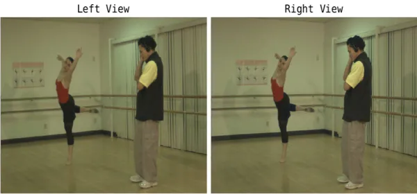
The least complex and the most popular 3D video format is the conventional stereo video (CSV). It is represented by two views (two color videos) of the same scene with a certain differenced angle of view. After capturing the scene with two cameras, video signals are processed under normalization, color correction,

rectification etc. Then, since it does not provide scene geometry information, captured video signals are directly displayed on a 3D display. Figure 2.3 shows an example of a stereo image that is captured by two cameras for CSV.

The algorithms of CSV are the least complex as it is mentioned since two steps are necessary: encoding and decoding the multiple video signals. The only difference between 2D video and CSV is the amount of data processed. However, the amount can be fixed by degradation of resolution.

Figure 2.3: CSV - left and right view. (ballet sequence is used by the courtesy of Interactive Visual Media Group at Microsoft Research.)

The coding and encoding algorithms are not going to be explained because the focus of this thesis is the choice of an appropriate 3D video representation format. CSV is not suitable for our system, since it does not represent a depth and geometry information of the system. However, the thumbnail of CSV can be generated by traditional methods such as automatic retargeting, scaling or cropping.

2.3.2

Video Plus Depth (V+D)

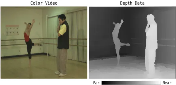
The next 3D video format is video plus depth (V+D) which provides a color video and an associated depth map data that stands for geometry-enhanced information of the 3D scene. The color video is similar with one of the views of CSV and the depth map is a monochromatic, luminance-only video. The depth range changes between two extremes: Znear as a 8-bit value 255 and Zfar as 0 that stand for the minimum and maximum distance of the corresponding 3D point from the camera respectively. Figure 2.4 shows an example of V+D.

Thus, for creating saliency-depth based 3D thumbnail generation, we use V+D format since it satisfies a depth map associated color video and is simple to use.

Figure 2.4: V+D - color video and depth map. (ballet sequence is used by the courtesy of Interactive Visual Media Group at Microsoft Research.)

2.3.3

Multiview Video Plus Depth (MVD)

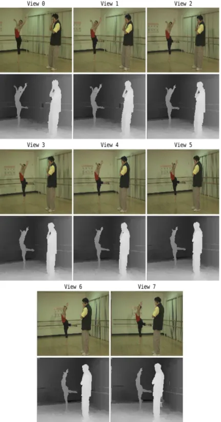
Multiview video plus depth (MVD) is an extension of V+D. As it is referred from its name, it has more than one view and associated depth maps for each views. This format is mainly used in free viewpoint applications, since it provides a number of different viewpoints. However, it is the focus of a new standardization

effort, which is dependent on the 3D display technologies and the goal of this format is to provide high-resolution videos, thus the complexity of MVD is high. Figure 2.5 shows an example of MVD format with eight views.

2.3.4

Layered Depth Video (LDV)

Layered depth video(LDV) is an alternative to MVD and extension of (V+D). Like V+D, it uses one color video with associated depth map. On the other hand, an extra component called background layer and the associated depth map of this layer is also used by LDV. The background layer is an image content which has foreground objects on it, as illustrated in Figure 2.6.

Figure 2.5: MVD with 8 views. (ballet sequence is used by the courtesy of Interactive Visual Media Group at Microsoft Research.)

Figure 2.6: LDV format. (ballet sequence is used by the courtesy of Interactive Visual Media Group at Microsoft Research.)

Thumbnail Generation System

3.1

System Overview

Our 3D thumbnail generation system is used to create 3D thumbnails from differ-ent types of 3D media such as 3D synthetic scenes and 3D natural videos. General architecture of the proposed system is shown in Figure 3.1. The system has four main components: Content Analysis, object ranking, transformation modeling and 3D rendering. The content analysis step is used to analyze the content, as explained in Section 3.1.1. In the next step, objects are ranked, and an im-portance map is extracted (Section 6.1.2). After the ranking process, objects are placed and scaled according to their importance (Section 3.1.3). Finally, for enhancing the depth perception, 3D rendering effects are applied to 3D meshes (Section 3.1.4).

Figure 3.1: General 3D thumbnail system.

3.1.1

Content Analysis

The first part of the system is the content analysis. It is executed differently according to the input type. For 3D videos, the selected frame is segmented into regions by mean-shift segmentation[13] in order to identify and process objects on the input image.

On the other hand, for 3D graphical contents, the best viewpoint of the scene is selected in order to give more information of the scene. Viewpoint entropy[59] is used to calculate the best viewpoint. The overview of this step is shown in Figure 3.2.

Figure 3.2: Content analysis.

3.1.2

Object Ranking

The second step is object ranking. In this level, the importance values of the objects in the scene or the segmented image are assigned and an importance map is created. As the previous step, it is processed differently for 3D videos and 3D graphical contents,as illustrated in Figure 3.3. For 3D videos, we use saliency and depth based methodology in furtherance of finding the importance of each object. While the saliency has been proposed to locate the points of interest, depth is

also another factor to decide whether an object is important or not. In other words, closer objects should be more salient due to proximity to the eye position. Therefore, we also use the depth map in order to assign importance values of objects for 3D videos. Furthermore, for 3D graphical scenes, this process is different. Since there are a lot of factors of affecting the importance of 3D meshes of 3D graphical contents such as size, dimension, mesh saliency, depth etc., we leave the determination of the importance values to the user. In such manner, for 3D graphical contents, user should assign the importance values of the objects.

Figure 3.3: Object ranking.

3.1.3

Transformation Modeling

In the transformation modeling step, the position and scale of important objects that appear on the thumbnail are determined. For 3D videos, the process is different from 3D graphical scenes because image retargeting is applied to the selected frame of the input video. On account of 3D videos, essential objects are extracted from the segmented image which is based on the importance map. Then, the resulting gaps are filled on the background. After pasting of important objects on the retargeted image, 3D mesh is created by using the associated depth map. For 3D graphical scenes, only the scales and positions of important objects

are determined with the importance map. Figure 3.4 shows the transformation modeling step.

Figure 3.4: Transformation modeling.

3.1.4

3D Rendering

The last step’s aim is to enhance depth perception by using 3D effects while rendering 3D thumbnails. Firstly, we use shadow mapping technique since the effect of shadows according to light source, background and viewpoint is useful for aiding the shape and depth perception (Figure 3.5-a). Besides, the parallax mapping (Figure 3.5-d) is applied in order to provide the parallax effect and for selection of thumbnails, we use Gooch shading (Figure 3.5-b). For more information on enhancing depth perception, see [12].

Thumbnail For 3D Graphical

Scenes

4.1

Overview

In this chapter, we present the first subsystem that generates 3D thumbnails for 3D graphical scenes. We assume that the input 3D scene satisfies the following conditions:

• The geometry of the scene is known.

• The model of the scene should be upright when loaded. • The scene should not be a closed scene.

• 16 viewpoints that are above the scene are chosen. The number and the

position of views can be changed by the user.

• The distance of the camera is set to a default value, but it may be adjustable

by the user.

The organization of this chapter is as follows: Section 4.2 explains the best viewpoint selection approach, Section 4.3 provides information about object rank-ing and transformation modelrank-ing is described in Section 4.4. Finally, Section 4.5 concludes this chapter with initial results.

4.2

Content Analysis

4.2.1

Best Viewpoint Selection

In this step, we compute the best viewpoint selection for each object on the input 3D graphical scene.

4.2.1.1 Viewpoint Entropy

We have used V´azquez’s approach[59] in our work. It is based on a metric that allows measuring the good viewpoint of a scene from a camera position, which is called viewpoint entropy. This metric refers to the amount of information cap-tured from a point on projected areas of faces. Thus, the best viewpoint is the one with maximum viewpoint entropy[59]. Viewpoint entropy has been demon-strated in many areas such as scene understanding and virtual world exploration, for calculation of suitable positions and trajectories for a camera exploring a vir-tual world [6][5][43][2][60]. It has also been used for Monte Carlo radiosity and global illumination to improve the scene subdivision in polygons; for the adap-tive ray casting [32][17][46]; and for image-based modeling to compute a minimum optimized set of camera positions.

To define viewpoint entropy, V´azquez uses the basics of the Shannon Entropy. This metric is described below.

Shannon Entropy

Theory of Communication[50]. In this approach, a discrete information known as

Markov process is firstly represented; and a new metric that is measurable and holds the quantity of the information is proposed.

The starting point of this metric comes from the following induction[50]:

“Suppose we have a set of possible events whose probabilities of oc-currence are p1, p2, ..., pn. These probabilities are known but that is all we

know concerning which event will occur. Can we find a measure of how much choice is involved in the selection of the event or of how uncertain we are of the outcome? ”

Denoting such a measure by the function H(p1, p2, ..., pn), three requirements that should be satisfied are listed [42]:

1. Continuity: H(p, 1− p) is a continuous function of p. 2. Symmetry: H(p1, p2, ..., pn) is a symmetric function.

3. Recursion: For every 0≤ λ < 1, the recursion H(p1, ..., pn−1, λpn, (1− λpn)) =

H(p1, ..., pn) + pnH(λ, 1− λ) holds. The illustration of this requirement is shown in Figure 4.1[58]. In the left side of three possibilities are shown as

p1 = 1₂, p2 = 1₃, p3 = 1₆. In addition to this, as it is illustrated in the right

side of the figure, firstly, between two possibilities each with probability 1₂ is chosen and if the second probability occurs, make another choice with probabilities of 2₃,1₃. The final results have the same probabilities as before and the function is H(1

2, 1 3, 1 6) = H( 1 2, 1 2) + 1 2H( 2 3, 1 3). The coefficient is 1 2

Figure 4.1: Shannon’s third requirement[58].

The theorem is concluded as the function H which satisfies the three assump-tions above: H =−K n X i=1 pilogpi (4.1)

where K is a positive constant. This quantity is called Shannon entropy. Among a limited number of possibilities, it is the measure of information which is the impact of the selection.

Additionally, it is a metric of uncertainty or ignorance. As a result of this, for discrete random variable X with values X = {x1, x2, ..., xn}, the function of

H(X) is defined as follows: H(X) =− n X i=1 pilogpi (4.2)

where n =|X|, pi = Pr[X = xi] for i∈ 1, ..., n. V´azquez interchangeably uses the notation H(p) or H(X) for entropy, where p represents the probability distribu-tion pi. As −logpi represents the information associated with the result xi, the entropy gives the average information or the uncertainty of a random variable[58].

Hence, in order to calculate the quality of the view, Shannon entropy is applied to V´azquez’s proposed measure, viewpoint entropy. This measure is based on the

amount of geometric information of a scene from a viewpoint. He assumes that the scene/environment satisfies the following conditions:

• Scene’s geometry is known.

• Scene is constructed by flat polygons.

• The words “face”, “polygon” and “patch” are referred to the same geometric

object. If the object is segmented into any smaller polygons or patches, each segmented patch or polygon is considered as a different face.

For V´azquez’s, the quality of the viewpoint is related to the amount of the information provided of a scene. Furthermore, the information satisfied from a viewpoint is dependent on the angle of the viewpoint to the faces of the scene. Thus, the good view is the one which holds the maximum information of the scene.

Definition

The basic work behind the definition of viewpoint entropy is Shannon entropy equation 4.2. For a given scene S, and a viewpoint p, the viewpoint entropy can be defined as follows: I(S, p) =− Nf X i=0 Ai At logAi At (4.3)

where Nf is the number of faces of the scene; Ai is the projected area of face I over the sphere; A0 stands for the projected area of background in open scenes;

and At is the total area of the sphere. Note that, when the scene is closed , A0

equals to 0. The visibility of face I is represented as Ai

At from point p. We can

only reach the maximum entropy when all faces with the same relative projected area (Ai

4.2.1.2 Computation of Viewpoint Entropy

We apply the viewpoint entropy on every object in the input scene. Since the best view of an object is the most informative one and holds the maximum viewpoint entropy, the steps for computation of viewpoint entropy for an object are as follows: Calculation of bounding sphere of the object, coding of the object by giving different RGBA colors to each face and the application of the Equation 4.3.

Bounding Sphere

In the first step, the object is surrounded by a bounding sphere as illustrated in Figure 4.2, and the camera is placed over a number of viewpoints on this sphere. The calculation of the bounding sphere is as follows:

• Find the minimum and maximum vertices of the object.

• Find the center of the bounding sphere by getting the average of the sum

of minimum and maximum vertices.

• Find the radius of the bounding sphere as a scalar that defines the maximum

distance from the center of the sphere to any vertices of the object.

• Calculate the vertices and normals of the sphere.

Color Coding of Objects

In order to calculate the viewpoint entropy, the number of pixels covered for each visible triangle from a specific camera position on the bounding sphere (i.e. the projected area as in Equation 4.3) should be computed. There are three different methods for computing the projected area: OpenGL histograms, hybrid software and hardware histograms and occlusion queries[10].

OpenGL histograms analyze the color information of an image. For this method, it is required to give each face of the scene a different color. Since four RGBA color channels are used, the length of item table of four integer val-ues is 256 and this item table represents the number of pixels that are visible.

Thus, the main disadvantage of this method is the necessity of several numbers of rendering passes for a scene that has more than 255∗ 4(1020) triangles. However, the off-screen rendering can be achieved for complex scenes in interactive rates with powerful graphic cards.

Figure 4.2: The camera positions that represents viewpoints[58].

For highly complex scenes, OpenGL histograms are not flexible because more than one rendering passes are necessary. Thus, an alternative way to OpenGL histograms is the hybrid software and hardware histogram method. The buffer read operation is not a complex and expensive method in recent GPUs because of the new symmetric buses such as PCI Express. This new hardware technology allows us to get a histogram in only one rendering pass, by sending the whole complex object with each triangle color-coded to rendering. After buffer read operation, we can get information about color of the pixel data. Unlike OpenGL histograms, complex scenes that have up to 256∗ 256 ∗ 256 ∗ 256(4, 228, 250, 625) triangles can be processed in only one rendering pass.

The third method for calculating viewpoint entropy is processed with OpenGL’s occlusion queries. Occlusion queries are used in hidden surface re-moval; and with this method, the objects that are not visible should not be sent to rendering for optimization and efficiency. Besides, from a particular viewpoint,

the area of the visible triangles can be determined by this method since occlusion query returns the number of visible pixels. Using this method, with k number of triangles in an object, k + 1 rendering passes take place by sending the k -triangled object and each triangle independently to render process. However, when the number of triangles increases, the efficiency of this method decreases. Thus, it is not suitable for highly complex scenes.

Castello et al. [10] compares these three methods with 6 camera positions and 9 different models from the least to highest complexity by calculating the viewpoint entropy for each camera positions. The comparison takes place in two different machines with two families of graphics cards: NVIDIA and ATI. From the results of this work, the rendering passes of OpenGL histograms increases when the complexity increases. With hybrid software and hardware histogram only one rendering pass is needed even if the object is complex. In other words, this method has a low cost. However, the results from occlusion query are worse than results of hybrid software and hardware histograms because rendering passes increase proportionally with the complexity of the object. Figure 4.4 shows the comparison of three methods, which shows that the hybrid histograms have the best performance.

As a result, we use the hybrid software and hardware histograms in order to calculate viewpoint entropy since the comparison results show that it is the best and efficient way of determining entropy for complex scenes more than 100, 000 triangles. Thus, we need to assign each triangle of the scene a different RGBA color value. Figure 4.3 shows some complex objects with different color-coded faces.

Application of Viewpoint Entropy Equation

After rendering from several number of viewpoints on the bounding sphere and assigning each face of the object different RGBA values, the item buffer is read and viewpoint entropy is calculated by using equation 4.3. The whole process is shown in Algorithm 2.

Figure 4.5 shows the rendered scenes from different viewpoints on the bound-ing sphere.

Figure 4.3: Color-coded complex objects.

4.2.1.3 The Best Viewpoint Selection

After calculating the viewpoint entropy for each viewpoint, the best viewpoint of the object is selected. Algorithm 2 shows how to compute entropy from a set of viewpoints and select the best one. As it is mentioned before, our calculation is based on V´azquez’s viewpoint entropy equation (Equation 4.3) and the best viewpoint selection algorithm (Algorithm 1) and the entropy computation is done by hybrid software and hardware histograms.

Figure 4.6 shows some results of complex objects of the input scene and se-lected viewpoints from a set of 5 viewpoints and the last column of each row shows the best viewpoint.

Figure 4.4: Comparison of viewpoint entropy calculation methods[10].

Figure 4.5: Results of viewpoint selection by using entropy[59]. (From Pere Pau V´azquez. Reproduced with kind permission of AKA Verlag Heidelberg from the Proceedings of the Vision Modeling and Visualization Conference 2001 ISBN:3-89838-028-9.)

Algorithm 1 Computes the view with the highest entropy of an object[58].

Select a set of points placed in regular positions on a bounding sphere of the object.

maxI ← 0 viewpoint ← 0

for all the points do

aux ← Compute the viewpoint entropy

if aux > maxI then

maxI ← aux

viewpoint ← current points

end if end for

Write maxI and viewpoint

Algorithm 2 Computing viewpoint entropy for an object on the scene.

1. Assign each face of the object a different RGBA color. 2. For each viewpoint k from 0 to number of viewpoints do

2.1 entropy k ← 0

2.2. Render the object 2.3. Read the item buffer

2.4. Find the total projected area as A t

2.5. For each face i from 0 to number of faces of the object do 2.5.1. Find the projected area of the face as A i

2.5.2. Apply Equation 4.3 2.5.3. Add result to entropy k

Figure 4.6: Figure (a), (b), (c), and (d) show rendered objects from a set of viewpoints. Figure (d) illustrates the best viewpoints.

4.3

Object Ranking

For 3D graphical scenes, object ranking is realized by the user. There are a lot of factors that affect the importance of 3D meshes such as size, dimension, mesh saliency, depth etc., and these issues are out of this thesis’s focus. Thus, the user gives the importance value between 0.0 and 1.0. The object has a value of zero is not displayed on the thumbnail and the most important object has a value of 1.0.

4.4

Transformation Modeling

After the selection of the best viewpoint of each object on the scene, objects are scaled and placed according to their importance values.

4.4.1

Scaling

Determining the scale of each object on the 3D graphical scene is one of the key issues. Our algorithm for scaling starts with the most important object for maximizing the functionality of them. Scales of important objects are maintained according to their importance values. In other words, the most important object is the biggest object on the thumbnail.

Algorithm 3 shows our approach for the computation of the scales of each object. The algorithm greedily scales them, beginning with the most important object. The variables used in this algorithm are defined as follows:

• width, height: The width and height of the object’s bounding box. • xScale, yScale: The scale over the x and y axes.

• thumbnailWidth, thumbnailHeight: The width and height of the generated

thumbnail’s bounding box.

• scale: The overall scale of the object.

• importance: The importance value of the object defined by the user between

0.0 and 1.0.

Algorithm 3 Computing the scale of important objects.

1. For each object m from the most important to least important do 1.1 Find the bounding box of object m as bBox

1.2 width ← width of bBox 1.3 height ← height of bBox

1.4 Calculate xScale as thumbnailWidth / width 1.5 Calculate yScale as thumbnailHeight / height 1.6 If xScale < yScale

1.6.1 scale ← xScale 1.7 else

1.7.1 scale ← yScale

1.8 Calculate the scale according to object’s importance 1.8.1 scale = (scale * importance )/nbOfObjects

For each object in the scene, the first step is to find the bounding box of the object. Then, the scale over the x and y axes are determined. From these values, the smallest one is selected in order to have a distorted mesh. After that, the scaling amount is calculated according to a simple function as illustrated in the step 1.8.1 (Algorithm 3) by using the assigned importance value of the object.

Figure 4.7 displays the results of our scaling algorithm for an aircraft and a mill.

Figure 4.7: Scaling results.

4.4.2

Positioning

After the determination of the scales of the objects, they are placed on the thumb-nail according to their importance values. As the order in the algorithm that is used for scaling, the process takes place in the decreasing order of importance. The object that has the highest importance value is the biggest, foremost and leftmost object for our work. Subsequent objects are placed in a layout from left to right and front to rear as illustrated in Figure 4.8.

Figure 4.8: Positioning layout.

Algorithm 4 shows the computation of the position of each object that appears on the thumbnail. The algorithm greedily places each object, beginning with the one with the largest importance. The variables used in this algorithm are defined as follows:

• scale: The scale of the object.

• transX, transY, transZ : Translation amounts on the x, y and z axes. • transXPrev, transZPrev: Translation amount on the x-axis and z-axis of

the previous object.

• thumbMinX, thumbMinY, thumbMinZ : The bounding box of the

thumb-nail’s minimum x, y, z value in terms of vertices.

• bBoxMinX, bBoxMinY, bBoxMinZ : The bounding box of the object’s

min-imum x, y, z value in terms of vertices.

• widthPrev, depthPrev: Width and depth of the previous object.

Algorithm 4 Computing the position.

1. For each object m from the most important to least important do 1.1 Find the bounding box of object m as bBox

1.2 Find the initial scale as scale from Algorithm 3 1.3 If m is the first object

1.3.1 transX ← thumbMinX - bBoxMinX 1.3.2 transY ← thumbMinY - bBoxMinY 1.3.3 transZ ← thumbMinZ - bBoxMinZ 1.4 else

1.4.1 transX ← transX_prev + widthPrev 1.4.2 transY ← thumbMinY - bBoxMinY 1.4.3 transZ ← transZ_prev - depthPrev

1.5 If bBox overflows the thumbnail’s box on the x-axis 1.5.1 transX ← thumbMinX - bBoxMinX

1.6 If bBox overflows the thumbnail’s box on the z-axis 1.6.1 Change scale to scale = (1.0 - trial) * scale

of each object

1.6.2 Restart the algorithm

For each object in the scene, the bounding box and the initial scale of the object is computed by using Algorithm 3. Then, the translation values on the x,y and z axes are determined. The displacement algorithm proceeds from left to right in the descending order of the importance value of the objects in the scene. If one of the object is out of the thumbnail box on the x-axis, the object is taken to the leftmost side of the box behind the previous objects. Moreover, if one of the object is out of the thumbnail box on the z-axis, all objects’ scales are reduced by a specific ratio and the algorithm is restarted from the scratch with the recent calculated scaling amount.

We have followed the displacement algorithm from left to right, since the leftmost objects are more salient than the right ones.

4.5

Results

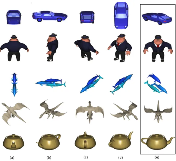
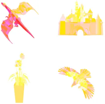
Figure 4.9: 3D thumbnails.

Figure 4.9 shows some results of our 3D thumbnail generation system for 3D graphical scenes. Cars, aircrafts, humans, animals, plants and houses are cate-gories that are represented in each thumbnail respectively. Moreover, Table 4.1 contains detailed information of 3D thumbnails illustrated in Figure 4.9. Number of models, vertices and faces that are displayed on the thumbnail are given in the Table 4.1.

Table 4.1: Model summary used in 3D thumbnails

Category Nb of Models Vertices Faces

Cars 2 5823 10142 Aircrafts 2 169085 295007 Humans 2 27457 48629 Animals 4 13380 26369 Plants 3 12938 14633 Houses 3 1824 3039

Thumbnail For 3D Videos

In this chapter, we present the second subsystem that generates 3D thumbnails for 3D videos + depth.

The organization of this chapter is as follows: Section 5.1 gives an overview of our system and Section 5.2 summarizes the selected 3D video format. Section 5.3 explains the content analysis step. Section 5.4 provides information about ob-ject ranking and transformation modeling is described in Section 5.5. Finally, Section 5.6 concludes this chapter with initial results.

5.1

Overview

The input of the framework is the selected video frame of a 3D video + depth as the RGB color map and the corresponding depth map of this frame.

Figure 5.1: Overview of the 3D thumbnail generation for 3D videos.

Figure 5.1 shows our approach for 3D thumbnail generation for 3D videos + depth. The input color map is first segmented into regions in order to calculate each regions’ importance, as explained in Section 5.3 and 5.4.1.Then, our method removes the important parts of the image, later to be exaggerated, and fills the gaps of the background using the technique described in Section 5.5.1. After-wards, the filled background is resized to standard thumbnail size of 192 x192. Then, important regions are pasted onto the resized background, as explained in Section 5.5.2. The final 3D thumbnail is generated by constructing a 3D mesh, as described in Section 5.5.3.

5.2

Selected 3D Video Format

As described in Chapter 2, a number of 3D imaging and video formats have recently been investigated. These formats can be roughly classified into two classes: N-view video formats and geometry-enhanced formats. The first class of

formats describes the multi-view video data with N views. For stereoscopic (two-view) applications, conventional stereo video (CSV) is the most simple format.

In the second class of 3D formats, geometry-enhanced information is added to the image. In the multi-view video + depth format (MVD) [52], a small number of sparse views is selected and enhanced with per pixel depth data. This depth data is used to synthesize a number of arbitrarily dense intermediate views for multi-view displays. One variant of MVD is Layered Depth Video (LDV), which further reduces the color and depth data by representing the common information in all input views by one central view and the difference information in residual views [39]. Alternatively, one central view with depth data and associated back-ground information for color and depth is stored in an LDV representation to be used to generate neighboring views for the 3D display. Geometry-enhanced formats such as MVD or LDV allow more compact methods, since fewer views need to be stored. The disadvantage however is the intermediate view synthesis required. Also, high-quality depth maps need to be generated beforehand and errors in depth data may cause considerable degradation in the quality of inter-mediate views. For stereo data, the Video + Depth format (V+D) is the special case. Here, one video and associated depth data is coded and the second view is generated after decoding.

Since the V+D format is more flexible for generating new views, the thumbnail representation is based on this format in this study.

5.3

Content Analysis

5.3.1

Video Frame Selection

There are several numbers of related works on video summarization and frame se-lection that are based on clustering-based[16], keyframe-based[40], rule-based[36]

and mathematically-oriented[21] methods. However, for our work, video summa-rization and frame selection issues are out of scope. Thus, we apply a saliency-based frame selection for our system. In this case, the saliency values of every frame of the input color video are computed and the most salient frame is selected in order to generate the 3D thumbnail. 3D videos are taken from FhG-HHI’s stereo-video content database[19].

Figure 5.2 shows some video frames, their saliency maps and the most salient frame.

Note that, the input color image/map refers to the selected video frame and the depth image refers to the depth map of the corresponding color map. Our method can be applied to single images with associated depth maps.

Figure 5.2: Saliency-based frame selection: Frame 0, 77, 103 and 211. The most salient one is the frame 103.

5.3.2

Image Segmentation

We use the mean-shift image segmentation algorithm for separating the input color image into regions. In addition to the mean-shift method [13], there are alternative segmentation methods such as graph-based [18] and hybrid segmen-tation approaches [41]. Pantofaru et al. [41] compares the three methods by considering correctness and stability of the algorithms. The results of this work suggest that both the mean- shift and hybrid segmentation methods create more

realistic segmentations than the graph-based approach with a variety of parame-ters. The results show that these two methods are also similar in stability. As the hybrid segmentation method is a combination of graph-based and mean-shift seg-mentation methods, it is more computationally expensive. Thus, we have chosen the mean-shift algorithm for its power and flexibility of modeling.

The mean-shift based segmentation method is widely used in the field of computer vision. This method takes three parameters together with the input image: spatial radius hs, color radius hr and the minimum number of pixels M that forms a region. The CIE-Luv color space is used in mean-shift algorithm, therefore the first step is to convert the RGB color map into Lαβ color space [38]. The color space has luminance, red-green and blue-yellow planes. These color planes are smoothed by Gaussian kernels.

Afterwards, for each pixel of the image with a particular spatial location and color, the set of neighboring pixels within a spatial radius hs, and color radius hr is determined and labeled. Figure 5.3 shows the image segmentation results for different values of hs, hr and M. In this work, we have chosen the parameters as shown in Figure 5.3-b.

For more information about mean-shift image segmentation, see Appendix A.

5.4

Object Ranking

5.4.1

Color and Depth Based Saliency Map

The next step computes an importance map from the input color and depth map. The aim of the retargeting algorithm is to resize images without losing the important regions on the input image. For this purpose, we calculate the importance of each pixel, as a function of its saliency in the color map and the depth map. We compute the saliency based on color and depth differently, as described below.

Figure 5.3: Mean-shift segmentation with different parameters. (a) Original Im-age; (b) hs = 7, hr = 6 and M = 800, number of regions: 31, 15, 19; (c) hs = 6,

hr = 5 and M = 50, number of regions: 214, 268, 246; (d) hs= 32, hr = 30 and

M = 150, number of regions: 1, 7, 6.

Computation of Saliency Based on Color Map

Most of the physiological experiments verify that human vision system is only aware of some parts of the incoming information in full detail. The concept of saliency has been proposed to locate the points of interest. In this work, we apply the graph-based visual saliency image attention model[23]. There are two steps for constructing the bottom-up visual saliency model: constructing activation maps on certain feature channels and normalization. This method is based on the bottom-up computation framework because in complex scenes that hold intensity, contrast and motion, visual attention is in general unconsciously driven by low-level stimulus.

Feature extraction, activation and normalization of the activation map are

• In the feature extraction step, the features such as color, orientation, texture,

intensity are extracted from the input image through linear filtering and the center-surround differences for each feature type are computed. In the classic algorithms, this step is processed by using biologically inspired filters.

• In the activation step, an activation map is formed from the feature maps

produced in step 1. A pixel with a high activation value is considered significantly different from its neighborhood pixels. At different scales such as henceforth, center, surround, the feature maps are subtracted in this step.

• In the last step, normalization of the activation map is performed, by

normalizing the effect of feature maps, and summing them into the final saliency value of the pixel based on the color map.

Figure 5.4: Graph-based saliency map. a) Original image; b) salient parts of the image (red - most salient); c) resulting saliency map.

Figure 5.4 shows sample results that are based on graph-based visual saliency image attention method. The detailed explanation of the algorithm can be found

in[23].

Computation of Saliency Based on Depth Map

We observe that depth is another factor to decide whether an object is of interest or should be ignored. In other words, closer objects should be more salient due to proximity to the eye position. Therefore, we also use the depth map to calculate depth saliency for each pixel in the input image. The function below for computing the depth importance map, adapted from the work of Longurst et al. [37], uses a model of exponential decay to get a typical linear model of very close objects. Therefore, in the equation, d and AD are constants to approximate the linear model by the overall rate of exponential decay where AD is 1.5 and d is 0.6: SD = 1 d√2π(exp− D2 d2 )AD (5.1)

Computation of Overall Saliency Map

For each region that was computed as the result of the earlier segmentation step, we compute the overall saliency of the region, by averaging the sum of the color-based and depth-color-based saliency of pixels belonging to the region.

5.5

Transformation Modeling

5.5.1

Background Resynthesis

The next steps after extracting important regions from the original color map are to resize the color map that has gaps to the standard thumbnail size, and to fill these gaps with the information extracted from the surrounding area. This step adopts Harrison et al. [24] inpainting method that reconstructs the gaps with the same texture as the given input image by successively adding pixels from the