Performance analysis of single structural break test with an empirical study on efficient market hypothesis"

(1)

"PERFORMANCE ANALYSIS OF SINGLE STRUCTURAL BREAK TEST WITH AN EMPIRICAL STUDY ON EFFICIENT MARKET HYPOTHESIS"

THE INSTITUTE OF ECONOMICS AND SOCIAL SCIENCES OF

BILKENT UNIVERSITY

The Institute of Economics and Social Sciences of

Bilkent University

by

İZZET YILDIZ

In Partial Fulfilment of the Requirements for the Degree of MASTER OF ARTS

in

THE DEPARTMENT OF ECONOMICS BİLKENT UNIVERSITY

ANKARA June 2005

(2)

I certify that I have read this thesis and have found that it is fully adequate, in scope and in quality, as a thesis for the degree of Master of Arts in Economics.

Asst. Prof. Taner Yiğit Supervisor

Asst. Prof. Ümit Özlale

Examining Committee Member

Asst. Prof. Aslıhan Altay-Salih Examining Committee Member

Approval of the Institute of Economics and Social Sciences

Prof. Erdal Erel Director

(3)

ABSTRACT

PERFORMANCE ANALYSIS OF SINGLE STRUCTURAL BREAK TEST WITH AN EMPIRICAL STUDY ON EFFICIENT MARKET HYPOTHESIS

Yıldız, İzzet Master of Economics Supervisor: Asst. Prof. Taner Yiğit

June, 2005

In this thesis, performance of the single structural break tests is examined. Since it has proved superiority of Sequential F test on other single break tests, it is chosen as single break test. Monte Carlo simulation is run for different scenarios and performances of the test with respect to estimating break points, and parameters, and rejecting or accepting the joint null hypothesis is observed. For all cases small sample bias is observed. The test estimates parameters correctly for large samples but for small samples it underestimates or overestimates parameters. Another common problem is about joint null hypothesis. When test rejects the joint null, it doesn’t identify which of the joint hypothesis is rejected. Therefore in this study, we utilize the t-statistic of the parameters to determine the individual hypothesis rejected. In addition to these common problems we illustrate other scenario specific problems in this study. We examine the implications of our Monte Carlo findings by applying the break test to real life data and investigate the efficient market hypothesis using stock market data on SP&500. Application of the sequential F test shows evidence against the efficient market hypothesis.

(4)

ÖZET

TEKLİ YAPISAL KIRILMA TESTİNİN VERİMLİ PİYASA HİPOTEZİ ÜZERİNDE AMPİRİK ÇALIŞMA İLE PERFORMANS ANALİZİ

Yıldız, İzzet

Yüksek Lisans, İktisat Bölümü Tez Danışmanı:Yrd. Doç. Dr. Taner Yiğit

Haziran, 2005

Bu tezde tekli yapısal kırılma testinin performansı incelenmiştir. Tekli yapısal kırılma testi olarak, diğer tekli yapısal kırılma testlerine üstünlüğü kanıtlandığı için, ardışık F testi seçilmiştir. Monte Carlo simulasyonları yapılarak çeşitli senaryolar hazırlanmış, ve bu senaryolarda testin kırılma noktasını ve parametreleri tahmin etmesine, boş hipotezi kabul veya red etmesine göre performansı incelenmiştir. Testin tüm durumlarda küçük örnekleme önyargısı gözlemlenmiştir. Test, büyük örneklemelerde parametreleri doğru tahmin ederken, küçük örneklemelerde düşük veya fazla tahmin etmiştir. Yapısal kırılma testinin diğer bir genel sorunu ise ortak boş hipotezlerin sınanmasıdır. Test ortak boş hipotezi red ederken, hangi hipotezi red ettiğini belirtmemektedir. Bu yüzden bu çalışmada hangi hipotezin red edildiğini belirlemek için parametrelerin t istatistikleri kullanılmıştır. Monte Carlo simulasyonları sonucundaki bulgularımızın anlamlılığını incelemek için kırılma testi, gerçek hayattan alınmış olan SP&500 borsa verileri üzerinde uygulanmış ve verimli piyasa hipotezi incelenmiştir. Ardışık F testi sonuçları, verimli piyasa hipotezine karşı kanıtlar göstermiştir.

(5)

ACKNOWLEDGMENTS

I would like to thank Asst. Prof. Taner Yiğit for his supervision and guidance through the development of this thesis. His patience and encouraging supervision brought my research up to this point.

(6)

TABLE OF CONTENTS

ABSTRACT...iii

ÖZET... iv

ACKNOWLEDGMENTS ... v

TABLE OF CONTENTS... vi

LIST OF TABLES ...viii

LIST OF FIGURES ... ix

CHAPTER 1:Introduction... 1

CHAPTER 2:Data and Methodology ... 4

2.1 Data Generation Process ... 4

2.2 Methodology: Sequential F test ... 5

CHAPTER 3:Results of Monte Carlo Simulation Under Different Scenarios ... 9

3.1 First Scenario: Data set is stationary and breaks are in both mean and trend... 9

3.2 Second Scenario: Data set is non-stationary and breaks are in both mean and trend... 12

3.3 Third Scenario: Data set is non-stationary and breaks are only in trend ... 15

3.4 Fourth Scenario: Data set is non-stationary and breaks are only in mean ... 18

3.5 Fifth Scenario: Stationary and non-stationary cases with no breaks... 20

3.6 Conclusion ... 23

CHAPTER 4:Empirical Study: Testing Efficient Market Hypothesis... 25

4.1 Introduction ... 25

4.2 Efficient Market Hypothesis ... 26

(7)

CHAPTER 5:Results of The Empirical Study... 30

5.1 Defining Lag Truncation Parameter... 30

5.2 Critical Value Determination ... 30

5.3 Results of Sequential Fmax Test... 31

5.3.1 Testing the whole sample... 31

5.3.2 Division of the Data Set ... 35

5.3.3 Testing Data set 1... 36

5.3.4 Testing Data set 2... 39

5.4 Conclusion ... 42

CHAPTER 6:Conclusion ... 45

(8)

LIST OF TABLES

1. Table 3.1 Results of Monte Carlo Simulations for Trend Break=0.06…………....…10 2. Table 3.2 Results of Monte Carlo Simulations for Trend Break=0.12………10 3. Table 3.3 Results of Monte Carlo Simulations for Trend Break=0.6…………..……11 4. Table 3.4 Results of Monte Carlo Simulations for the Second Scenario..…………...13 5. Table 3.5 Results of Monte Carlo Simulations for the Third Scenario………...….…16 6. Table 3.6 Results of Monte Carlo Simulations for the Fourth Scenario…………...18 7. Table 3.7 Results of Monte Carlo Simulations for the Fifth Scenario……..………...21 8. Table 5.1 Critical Values for the Sequential Maximum F Test...……….31 9. Table 5.2 Ordinary Least Square Estimation Results for the Sequential F Test…...34 10. Table 5.3 Ordinary Least Square Estimation Results for Data Set 1…………....….38 11. Table 5.4 Ordinary Least Square Estimation Results for Data Set 2………..…...…41

(9)

LIST OF FIGURES

1. Figure 5.1: Stock prices with respect to months………...………32

2. Figure 5.2: F values with respect to months………...………...32

3. Figure 5.3: Stock prices with respect to months………..…….……37

4. Figure 5.4: F values with respect to months ………...………….….…...37

5. Figure 5.5: Stock prices with respect to months ………...………...40

(10)

CHAPTER 1 INTRODUCTION

Unit root methodology is one of the most popular topics in the literature since unit root property is frequently observable in most of the economics data set. Because of this reason there is a large literature on this methodology. However structural breaks or in other words sudden and somehow persistent changes in time series because of wars, crises, policy changes etc..., are also observed in data sets frequently. And in the existence of structural breaks, classical unit root tests such as Dickey and Fuller (1979) t-statistics don’t give proper result about the unit root property. In his paper, Perron (1989) showed that when breaks exist Dickey and Fuller (1979) t-statistics fails to reject the null hypothesis of unit root too often for trend stationary data. Thus after the results of Perron (1989), studies focused on finding new unit root tests that are able to capture the structural breaks.

Starting point of the unit root test with structural breaks is also the paper of Perron (1989). In his paper, he presented three kinds of break model. 1) The crash model: allows break in intercept 2) The changing growth model: allows for break in the slope 3) The mixed model: allows for break both in intercept and in slope. For the subsequent structural break test literature, these models set the benchmarks. Perron proposed a methodology which was a motivation for the other break studies. He first determined the place of the break point by deriving the limiting distribution of the t-statistics and then estimated the parameters of the model.

(11)

This methodology was a motivation point for other studies because since the limiting distribution of t statistic depends on the location of break which is taken as a priori, it is criticized by other researchers. These criticisms led to the increase the number of studies on structural breaks and unit roots. One of the most detailed ones is Banerjee, Lumsdaine, and Stock (1992). They mentioned that taking the break point as a priori may cause to reject the unit root too often and it will be biased. They assert that methods for choosing the break point must depend on the whole data. Therefore they proposed sequential t and F tests for determining the break point in data. Also Christiano (1992), Zivot and Andrews (1992), Perron and Vogelsang (1992), Perron (1997) emphasized the need for a pretest for determining the location of break and they proposed sequential minimum t test and sequential maximum F tests. Finally Sen (2003) developed the technique in Banerjee, Lumsdaine, and Stock (1992) by expanding the regressor matrix and he is able to test joint null hypothesis of no break in mean and trend, and unit root property at the same time.

Although the literature on the single break tests and joint test of a single break with unit root is sizeable, in most studies two types of the tests are commonly used. These are sequential minimum t tests and sequential maximum F test. Murray(1998) and Murray and Zivot(1998) studied the power of the tests for the joint null hypothesis of unit root and no trend and mean break. Their results showed that power of the sequential maximum F test is more stable and greater than the sequential minimum t-statistics. Because of this reason in this study I will focus on sequential F tests mentioned in Sen (2003). I will try to explain the properties of this sequential F test for both small samples and large samples. I will examine the accuracy of the test for both

(12)

parameter estimation and break points locating under different scenarios, for different amount of mean and trend breaks. Finally, I will apply sequential maximum F-tests on stock price data of United States, and comment on the efficient market hypothesis in different periods.

The study is organized as follows. Chapter 2 gives information about data generation process and methodology of the sequential maximum F test. Chapter 3 presents the results of Monte Carlo simulations under different scenarios and makes evaluations on the performance of the test about the sequential F test. Chapter 4 and chapter 5 are empirical study part. Chapter 4 gives information about literature on efficient market hypothesis and previous studies. Chapter 5 includes the results of the joint break tests including the unit root tests for different periods in the stock price data and the results on the test of the efficient market hypothesis. Finally, Chapter 6 gives a general conclusion about the properties and usage area of the structural break test.

(13)

CHAPTER 2 DATA AND METHODOLOGY

2.1 Data Generation Process

In this chapter, properties of the single structural break test, sequential maximum F test in Sen(2003) is examined. In order to investigate the properties Monte Carlo simulations with different scenarios are performed. These scenarios are prepared by using different data set which is generated by the same process with Sen ( 2003);

1 3 (1 ) c c t _t _t _t L y DU DT e α µ µ − = + + t=1,2……T (2.1) In this data generation process, α is the first order auto regression parameter and in order to examine the properties of the test in case of unit root, data set with α=1 is generated. For the stationary cases data sets with α=0, α=0.3 and α=0.6 is prepared with equation (2.1). Three different sample size, T=100, T=200 and T=400 are used.

c t

DU is defined as the proposed mean break date and c

t

DT as the proposed trend break date in the processes. Break dates are defined in middle of the sample as T/2. In equation (2.1)µ1 is

defined as the amount of the break in the intercept and µ3 is defined as the shift in the

slope. While preparing the joint break scenarios, I try to figure out amount of mean and trend breaks with respect to their powers. I define the power of break as increase or decrease it causes in the area below the line graph of data. By using this definition I formulate the power of the breaks as follows;

(14)

2

Power of Trend Break = ∆trend*(T−T_b) / 2 (2.2)

Power of Mean Break = ∆mean*(T−T_b) / 2 (2.3)

where Tbis defined as point of break in the sample. Then ratio of the break powers are

formulated to determine the size of trend breaks for given mean breaks:

Mean Break = 0.003*T (2.4) Ratio of Trend B./Mean B.(Power ratio) = (∆trend/∆mean) *(T−Tb) / 2 (2.5) Given sample sizes of 100, 200, 400 and using power ratios of 0.5, 1 and 5 mean and trend breaks are determined. For the stationary cases, following combinations of (µ1, µ3,

T) are used; (3,0.06,100), (6,0.06,200), (12,0.06,400), (3,0.12,100), (6,0.12,200), (12,0.12,400), (3,0.6,100), (6,0.6,200) and (12,0.6,400). For the unit root scenarios in joint break cases, following combinations of (µ1, µ3, T) are used; (3,0.0064,100), (6,0.0064,200), (12,0.0064,400), (3,0.0128,100), (6,0.0128,200), (12,0.0128,400), (3,0.064,100), (6,0.064,200), (12,0.064,400). Also in order to measure the performance of the joint break test for single break data sets, scenarios including single break of both trend and mean are prepared. Combinations of (µ1, µ3, T) in these processes are; (0, 0.12, 100), (0, 0.12, 400), (3, 0, 100), (3, 0, 400), (0, 0.12, 100), (0, 0.12, 100).

2.2 METHODOLOGY: Sequential F test

In order to test the non stationary, we must choose a unit root test. One of the most popular unit root test is Dickey and Fuller (1979) t-statistics. But Perron (1989) showed that Dickey and Fuller (1979) t-statistics accepts null hypothesis of unit root too often for trend stationary data in case of breaks. Since probability of breaks in stock

(15)

markets may be high because of crisis and bubbles in markets, testing data with Dickey Fuller statistics will be useless. Test statistics allowing breaks in testing unit root as sequential F and sequential t tests is offered by Banerjee, Lumsdaine, and Stock (1992). Therefore I choose sequential tests for this study. There are three kinds of model for the break tests in Perron (1989):

1) The crash model: allows break in intercept

t 0 1 t 2 t-1 t 1 y = µ + µ DU (T ) + µ t + y + + e k c b j t j j c y α − = ∆

∑

(2.6)

2) The changing growth model: allows for break in the slope

t 0 1 t 2 t-1 t 1 y = µ + µ DT (T ) + µ t + y + + e k c b j t j j c y α ₋ = ∆

∑

(2.7)

3) The mixed model: allows for break both in intercept and in slope

t 0 1 t 2 t 3 t-1 t 1 y = µ + µ DU (T ) + µ DT (T ) + µ t + y + + e k c c b b j t j j c y α − = ∆

∑

(2.8) where Tc

b is the correct break-date, DUt is for the mean break and DUt( T c

b ) = 1(t> T c b),

DTt is for the trend break and DTt( Tbc) = (t - T c b) 1(t> T c b ), and 1(t> T c b) is an indicator

function that takes on the value 0 if t = Tc

b and1 if t > T c

b . Also in equation (2.8), µ0 is

the mean value before the possible mean break, and µ1 represents the amount of changes

in mean break, µ2 denotes value of slope before the possible trend break, µ3 is the amount

of changes in trend break, and finally α is the auto regression parameter. In order to eliminate the correlation in disturbance term, k additional regressors (

1 k j t j j c y₋ = ∆

∑

) is

(16)

added in the model. The value of the lag truncation parameter (k) is taken as unknown and it must be estimated from data before running the model. Parameter k must be given as input to the model.

Murray(1998) and Murray and Zivot(1998) studied on the power of the tests statistics for the joint null hypothesis of unit root and no trend and mean break Their results showed that power of the sequential maximum F test is more stable and greater than the sequential minimum t-statistics. Because of this reason, I will use sequential F tests to examine breaks.

Sequential maximum F test statistics presented in Sen (2003) as:

1 1 2 1 ( ) ( ( ) ) *( *( ( ) ( ) ) ) *( ( ) ) / ( ) T t b b t b t b b b t F T Rµ T r R X T X T − R − Rµ T r qσ T = ′ ′ ′ = −

_∑

− (2.9)

where µ( )Tb is the ordinary least square estimator of µ =(µ µ µ µ α0, 1, 2, 3, , ,..., )c1 ck ′in

equation (2.9).

X T

t

( ) (1,

b

=

DU T

t

( ), ,

b

t DT T

t

( ),

b

y

t−1

,

∆

y

t−1

,....,

∆

y

t−k

)

′

and (0, 0,1)

r= ′ r is the restriction matrix. Restriction matrix depends on the type of the test. If we want to test unit root in case of trend and mean break, in another word if our null hypothesis

0 : 1, 1 0, 3 0

H α = µ = µ = , restriction matrix isr=(0, 0,1)′. In equation (2.9), q is the number of restrictions and it is equal to 3 for the null hypothesis H0. Variance is

equal to 2 1 2 1 ( ) ( 5 ) ( ( ) ( )) T b _t _t b b t T T k y x T T

σ

−

µ

= ′

= − −

∑

− and r is equal to R*µ. Since in this study our interest is on joint tests of both mean break, trend break and unit root, our null hypothesis is

0 : 1, 1 0, 3 0

(17)

R = 0 1 0 0 0 0 0 0 1 0 0 0 0 0 1 k k k O O O

where Ok is the zero row matrix with the truncation lag k.

In sequential F test, F values of the each point for the given interval is calculated by the formula in (2.9). Then the maximum of these F values are chosen and the location of this maximum F value is taken as the candidate for the break point. If maximum F value is greater than the critical values, we can reject the null hypothesis as Sen (2003) does.

(18)

CHAPTER 3 Results of Monte Carlo Simulation Under Different Scenarios

Model given in the chapter 2 for the structural break test and data generation process is coded in GAUSS. All simulations are done for 2000 replications and average of the parameters and t-statistics are used in the results. Performance of the break test is examined under five different scenarios.

3.1 First Scenario: Data set is stationary and breaks are in both mean

and trend

In this scenario data set is generated as stationary and breaks are located in the middle of the data (T/2) for both mean and trend. AR parameter and amount of trend and mean breaks are changed to observe the performance of the test in different situations.

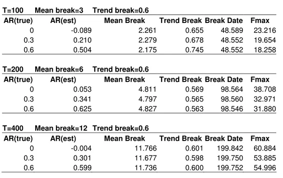
In Table 3.1, results of the test for trend break = 0,06 while AR parameter and mean break is gradually increasing is given. In Table 3.2 and Table 3.3 trend breaks are increased to 0,12 and 0,6 while AR parameters and mean break parameters are same as in Table 3.1.

(19)

Table 3.1 Results of Monte Carlo Simulations for Trend Break=0.06

T=100 Mean break=3 Trend break=0.06

AR(true) AR(est) Mean Break Trend Break Break Date Fmax

0 -0.089 3.177 0.066 48.997 22.312 0.3 0.220 3.251 0.068 49.034 17.788 0.6 0.530 3.336 0.073 49.038 14.125

0 0.068 5.402 0.056 98.723 35.910 0.3 0.354 5.353 0.056 98.706 29.054 0.6 0.637 5.305 0.054 98.659 24.637

T=400 Mean break=12 Trend break=0.06

0 -0.011 11.896 0.059 199.932 58.204 0.3 0.292 11.889 0.059 199.862 49.487 0.6 0.595 11.910 0.059 199.848 45.777

0 -0.084 3.093 0.131 48.962 22.132 0.3 0.214 3.166 0.136 48.980 17.922 0.6 0.529 3.235 0.144 48.949 14.138

0 0.065 5.341 0.112 98.694 36.030 0.3 0.355 5.278 0.111 98.661 29.216 0.6 0.635 5.267 0.109 98.657 24.853

0 -0.012 11.908 0.120 199.938 58.138 0.3 0.293 11.867 0.120 199.874 49.075 0.6 0.596 11.882 0.120 199.838 45.871

(20)

0 -0.089 2.261 0.655 48.589 23.216 0.3 0.210 2.279 0.678 48.552 19.654 0.6 0.504 2.175 0.745 48.552 18.258

0 0.053 4.811 0.569 98.564 38.708 0.3 0.341 4.797 0.565 98.560 32.971 0.6 0.625 4.827 0.563 98.546 31.880

0 -0.004 11.766 0.601 199.842 60.884 0.3 0.301 11.677 0.598 199.750 53.885 0.6 0.599 11.736 0.600 199.752 54.996

In all the cases given in Table 3.1, Table 3.2 and Table 3.3 F values are larger than the critical values at 1 percent significance level and null joint hypothesis, stationary with no mean and trend break, is rejected for all cases. Also break dates are estimated correctly as middle of the data set. Therefore sequential break test finds the break date correctly for the stationary cases and the mixed break model. In addition to this, structural break test estimated amount of breaks in trend and mean correctly. However estimation of trend parameters is estimated more accurately than mean parameters especially for small sample sizes as T=100. Another property of the structural break test is the that F values are increasing proportionally with T. For example maximum F values are doubled when T increases from 200 to 400. Therefore we can say that power of the test is increasing with T. For large samples, breaks are determined more easily. Another interesting property is that F values are not affected

(21)

from the amount of the trend breaks. For the same cases in Table 3.1, Table 3.2, and Table 3.3 only trend values are increased but f values are almost same. Finally, AR parameter estimation is accurate for the large sample sizes as T=400, but its accuracy is lower in small samples. For example in Table 3.3 for AR (true) =0.6 and T=100, break test estimated this parameter as 0.5 but when T increases to 400, test estimated AR parameter as 0.599 which is definitely same as the real value. In general performance of the test under this scenario is well since all parameters and breaks are estimated correctly, and their dates found as they are proposed.

3.2 Second Scenario: Data set is non-stationary and breaks are in both

mean and trend

Another situation which is important for the performance of the test in the real data applications is unit root cases. In order to evaluate the test, data set of scenario is generated as non-stationary and breaks are located in the middle of the data (T/2) for both mean and trend.

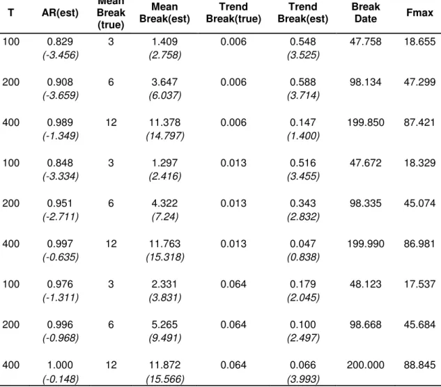
In Table 3.4, t-statistics are also calculated and given in italics in the second lines. For three different sample sizes, mean breaks and trend breaks totally 9 cases are simulated and results of these cases are given in Table 3.4.

(22)

Table 3.4 Results of Monte Carlo Simulations for the Second Scenario T AR(est) Mean Break (true) Mean Break(est) Trend Break(true) Trend Break(est) Break Date Fmax 100 0.829 3 1.409 0.006 0.548 47.758 18.655 (-3.456) (2.758) (3.525) 200 0.908 6 3.647 0.006 0.588 98.134 47.299 (-3.659) (6.037) (3.714) 400 0.989 12 11.378 0.006 0.147 199.850 87.421 (-1.349) (14.797) (1.400) 100 0.848 3 1.297 0.013 0.516 47.672 18.329 (-3.334) (2.416) (3.455) 200 0.951 6 4.322 0.013 0.343 98.335 45.074 (-2.711) (7.24) (2.832) 400 0.997 12 11.763 0.013 0.047 199.990 86.981 (-0.635) (15.318) (0.838) 100 0.976 3 2.331 0.064 0.179 48.123 17.537 (-1.311) (3.831) (2.045) 200 0.996 6 5.265 0.064 0.100 98.668 45.684 (-0.968) (9.491) (2.497) 400 1.000 12 11.872 0.064 0.066 200.000 88.845 (-0.148) (15.566) (3.993)

Note: Numbers in parenthesis are calculated t statistics for estimations. In t statistics, for mean and trend break no break case and for AR unit root is taken as null hypothesis

There are some similarities as in the first scenario observed before. First, break dates are found in their true location, the middle of the sample size. Another similar result is that F value is increasing with sample size T which is an evidence for that the test is more powerful in large samples.

(23)

In all cases, F values are significantly greater than the critical values and so null hypothesis of non stationary with no mean and trend break is rejected. But in this case we can not conclude that whether the reason of rejection is stationarity or breaks in trends and means or both. Because of this reason we also calculated t-statistics for the parameters of the model which is given also in Table 3.4. One of the interesting results is that accuracy of the AR parameter estimation increases with T. When T increases from 100 to 400, estimation of AR parameter converges to 1. Also when T increases also t-statistics of the AR parameter decreases, which means that for large T estimate of parameter is not significantly different than 1. Therefore we can conclude that for large samples model estimates AR parameter correctly, while for small T the model underestimates AR parameter under this scenario.

For the mean break parameter estimates, all t-statistics are significant at 1 percent level and we can say that amount of break is significantly larger than 0. Estimation values of mean break parameters for small samples as T=100 and T=200 are also underestimated in all cases. But for large samples as T=400, break test estimated values of mean break parameters correctly as they are set.

For trend break parameters performance of the test is not so good. Break test couldn’t estimate correct values for all of the cases (except T=400 trend break=0.064) and t-statistics for these cases are not consistent. In some cases, as T=200 and trend break=0.006, they are significant at 1 percent level while in some others, as T=400 and trend break= 0.013, they are not significant. One common factor observed in Table 3.4 is that distance between the correct values of the trend break and its estimation is getting closer as T increases. This is likely due to the increasing power of large sample sizes.

(24)

The only logical result for trend breaks is for the last case of T=400 trend break=0.064. In this case trend break parameter is estimated correctly as 0.066 but at the same time its t-statistic is significant at 1 percentage level. So we can conclude that performance of the test for trend breaks is not as good as its performance in mean breaks under this scenario. For small samples sizes and small amount of trend breaks, estimation of trend breaks is far away from their correct values.

Another important result for this scenario is that magnitude of F values is affected from only sample size T. Maximum F value is robust to the amount of trend breaks. For example, maximum f values of the simulations with sample size 100 and trend breaks of 0.006, 0.013, and 0.064 are 18.655, 18.329, and 17.537 respectively. F values are not changing with respect to trend breaks. However maximum f values for trend break of 0.006 and sample size 100, 200, and 400 are 18.655, 47.299, and 87.421 respectively. F values are sensitive to sample size and increasing with T.

3.3 Third Scenario: Data set is non-stationary and breaks are only in

trend

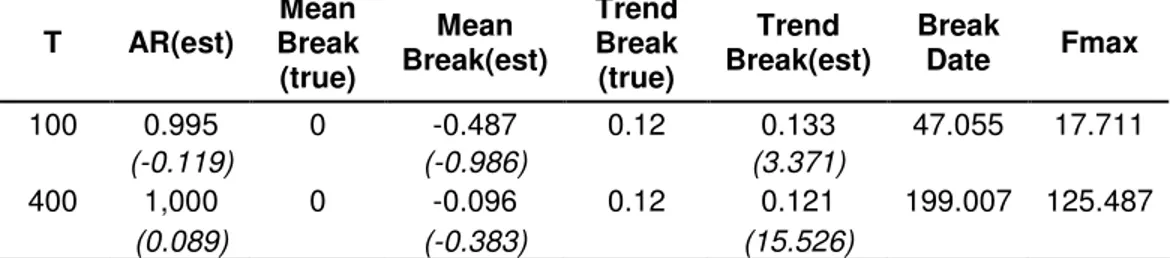
Another research area for the performance of the test is non stationary cases with only trend breaks. This scenario is necessary to investigate whether there is an influence of the mean break on trend break under scenario 2 and also to examine performance of the test for pure trend breaks. Data is generated with unit root and the trend break is set in the middle of the sample. Two sample sizes are used. T=100 is used to symbolize the small samples and T=400 is used to symbolize large samples. Results of the simulations are given in Table 3.5.

(25)

Table 3.5 Results of Monte Carlo Simulations for the Third Scenario T AR(est) Mean Break (true) Mean Break(est) Trend Break (true) Trend Break(est) Break Date Fmax 100 0.995 0 -0.487 0.12 0.133 47.055 17.711 (-0.119) (-0.986) (3.371) 400 1,000 0 -0.096 0.12 0.121 199.007 125.487 (0.089) (-0.383) (15.526)

Like in all other scenarios break dates are estimated correctly in the middle of the samples for both cases and maximum F values are significant at 1 percent level and null hypothesis of nonstationary with no mean and trend break is rejected. Again there is the critical question why test rejected the null hypothesis, because of break in trend or stationarity in data. Unfortunately break test couldn’t give a certain answer for this question, and the only thing we can do is to derive t-statistics to help us comment on that issue.

If we examine t-statistics given in parenthesis in Table 3.5, we can observe that values of t-statistics for AR estimation parameters are larger than Dickey Fuller critical values, meaning that AR estimation parameters are not significantly different than 1. Also value of the estimation for small sample size T=100 is 0.995 and for the large sample size T=400 is 1. Therefore by looking estimation values and t-statistics, we can say that nonstationarity is caught by the structural break test.

Since the data is generated without a mean break, we expect the simulations not to catch any mean breaks. This is confirmed in Table 3.5, absolute values of t-statistics of mean breaks are smaller than the critical values of the t distribution. If we look the estimated values they are -0.487 for small sample T=100 and -0.096 for the large sample

(26)

T=400 and they are not significantly different than 0. Also here small sample size property is again observed. Since absolute value of the t-statistics is smaller and the estimation value are almost zero for T=400, we can say that structural break test is more powerful for large samples.

Critical point under this scenario is the estimation of the trend values. As we can remember while there is also mean break in nonstationary case as in second scenario, break test couldn’t estimate trend values correctly. When we removed the mean break in this scenario, performance of the test for estimation of trend break increased significantly. If we notice the t-statistics for the trend break in Table 3.5, they are 3.371 for small sample T=100 and 15.526 for large sample T=400. These values are larger than the critical values given in t distribution tables at 1 percent significance level. Therefore we can say that trend breaks are significantly different than zero. In addition to the t-statistics estimated values of the trend break parameters are close to their true values.

Break is proposed as 0.12 and estimated value for small sample is 0.133 and for larger one is 0.121. Here again we can observe the effect of small sample size property. For small samples, estimation is not close to the correct values as they are in large samples and t-statistics are smaller than the ones in large samples. But in spite of small sample size property for both cases, different than the scenario 2, break test estimated the trend break accurately. This implies very important result for the structural break test, namely under the nonstationary case existence of mean break lowers the performance of the test while estimating the trend break. If the mean break is removed, performance of the break test estimating the trend break increases significantly.

(27)

3.4 Fourth Scenario: Data set is non-stationary and breaks are only in

mean

After examining performance of the test in nonstationary cases with only trend breaks, another interesting area will be the nonstationary cases with only mean breaks. As we noticed from the previous scenarios performance of the test for detecting trend break is being affected by the presence of the mean break. In order to find out whether mean breaks have an impact on break tests, we generate data with unit root and the mean break is set in the middle of the sample. As in scenario three, two sample sizes are used. T=100 is used to symbolize the small samples and T=400 is used to symbolize large samples. Results of the simulations are given in Table 3.6.

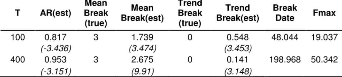
Table 3.6 Results of Monte Carlo Simulations for the Fourth Scenario

T AR(est) Mean Break (true) Mean Break(est) Trend Break (true) Trend Break(est) Break Date Fmax 100 0.817 3 1.739 0 0.548 48.044 19.037 (-3.436) (3.474) (3.453) 400 0.953 3 2.675 0 0.141 198.968 50.342 (-3.151) (9.91) (3.148)

Like in other scenarios again break dates are estimated correctly as in the middle of the samples for both cases and maximum F values are also significant at 1 percent level and null hypothesis of nonstationary with mean break and no trend break is rejected. As in the third scenario the same problem occurs again; we can not answer the question why test rejected the null hypothesis. We can not definitely know from the results whether it is because of break in mean or stationarity in data. Therefore again the

(28)

only thing we can do is to derive statistics and comment on that issue by the help of t-statistics.

If we examine statistics given in Table 3.6, we can observe that values of t-statistics for AR estimation parameter are significant at 5 percentage level with respect to the critical values given in Dickey Fuller table which means that AR estimation parameters are significantly different than 1. This result of the break test is wrong since data generation process of our model sets the AR parameter as 1. This is another interesting result of the structural break test that needs to be noticed. This problem is not observed in scenario three where there is only trend break and in that case t-statistics of the break tests are not rejecting unit root for the nonstationary data. But under this scenario with only mean break, t-statistics are rejecting unit root for the nonstationary data. On the other hand, value of the estimation for small sample size T=100 is 0.817 which is far away from 1, and for the large sample size T=400 is 0.953 which is less accurate than its similar case in scenario three. Therefore for scenario four by looking at estimation values and t-statistics, we can say that nonstationarity couldn’t be detected by the structural break test.

Another interesting point, despite there is no trend break in the data generation process, trend break values that comes out of the simulations regards for cases in Table 3.6, absolute values of t-statistics of trend breaks are significant at 1 percentage level. If we look at the estimated values they are 0.548 for small sample T=100 and 0.141 for the large sample T=400 and they are different than 0. The small sample size property is again observed since absolute value of the t-statistics and the estimation values are closer to zero for T=400. Therefore we can conclude that performance of break test

(29)

detecting the trend break while there is a mean break is low which is also observed during the evaluations in second scenario.

Another critical point under this scenario is the estimation of the mean values. As we can remember in previous scenarios break test estimates mean break values correctly. Since we don’t know what the break test rejected, whether stationarity or mean break; we must examine t-statistics values. If we examine the t-statistics for the mean break in Table 3.6, they are 3.474 for small sample T=100 and 9.910 for large sample T=400. These values are larger than the critical values given in t distribution tables at 1 percent significance level. Therefore we can say that mean breaks are significantly different than zero. In spite of t-statistics estimated values of the mean break parameters are not close to their preset values especially for small samples. Although proposed mean break value is 3, estimated mean break value for is 1.739 T= 100 and 2.675 for T=400. Especially for the small sample T= 100 estimated value is far away from the proposed value. But as T increases estimations are getting closer to the proposed value. This can be because of the power increase due to the larger sample sizes.

3.5 Fifth Scenario: Stationary and non-stationary cases with no breaks

Up to this point we consider stationary and nonstationary cases separately. In this scenario, our goal is to observe the performance of the test in detecting the stationarity of the data set for different sample sizes.

(30)

Table 3.7 Results of Monte Carlo Simulations for the Fifth Scenario T AR(true) AR(est) Mean Break (true) Mean Break(est) Trend Break (true) Trend Break(est) Break Date Fmax 100 1 0.773 0 0.024 0 0 49.733 6.739 (-3.765) (0.051) (0.016) 400 1 0.939 0 -0.007 0 0 197.406 6.510 (-3.807) (-0.034) (0.008) 100 0.9 0.709 0 0.008 0 -0.001 49.958 7.219 (-4.179) (0.017) (-0.05) 400 0.9 0.852 0 -0.01 0 0 195.913 10.794 (-5.566) (-0.043) (0.014)

Unlike the other scenarios while generating the data set, breaks are not allowed in order to examine the performance of the test for pure unit root and stationary cases. For the first two cases, since properties of the data set is the same with the null hypothesis of our break test which is the nonstationarity and no break in trend and mean, maximum F values are also average of the critical values. In the second case the only difference is the change in the AR parameter. And comparing the maximum F values, we can notice the increase in both cases. This is the sign of the break test detecting nonstationarity test. Also small sample size property is observed in this situation. Since the increase in the F value for large sample is much greater than the one in the small sample. In any case, we can say that by looking the F values break test detects a difference between stationary and nonstationary cases. We inspect the other parameters and their t-statistics to investigate these differences.

If we look at the t-statistics for the mean and trend break parameters, we can notice that for all cases their absolute vales are smaller than the critical values given in t distribution table and so they are insignificant. Since the null hypothesis of these t-statistics is no break in parameters, we conclude that there is no evidence for any break.

(31)

In addition to this, estimations of parameters are around the zero, which is supporting the conclusion of no break.

Since there is no break in mean and trend parameters, increase in maximum F values of the last two cases must be because of detecting the stationarity in the data set. In order to prove this fact, we must also examine the t-statistics for the AR parameters. For all the cases, t-statistics are larger than the critical values given in the Dickey Fuller table at 1 percentage level. Since the null hypothesis for the t-statistics is unit root, by rejecting the null hypothesis with t-statistics for all cases we also reject that AR parameter is equal to 1. But if we look t values carefully, we can observe that when generated data is stationary with AR=0.9, values of t-statistics are -4.179 and -5.566 for T=100 and T=400 and much smaller than the ones for the unit root cases (AR=1) which are -3.765 and -3.807 for T=100 and T=400. Therefore this can be the reason for increase in maximum F values. Test detects the changes in AR parameters with the increase in F values but it doesn’t distinguish so well between the AR parameters using the t-statistics.

Small sample size again impacts the estimates. While sample size is increasing estimation for AR parameters are getting closer to their true values. For example for the unit root case (AR=1), estimated AR value is 0.773 for T=100 and 0.939 for T=400. For T=400 estimated AR parameter is closer to the exact value of 1. Similar situation is valid for the stationary case too.

In conclusion, break test is successful for estimating no breaks in trend and mean and detecting the nonstationary with respect to the maximum F values. However, the t-statistics and the AR parameter estimates are less reliable in the case of small samples.

(32)

3.6 Conclusion

After running break test for five different scenarios, situations where break test performs well and situations where it fails are determined. Break test is performing quite well in certain aspects. These are mentioned below.

• Test is detecting the break dates accurately for every case.

• Maximum F values correctly reject cases that violate the joint null hypothesis of nonstationarity and no break in mean and trend.

• For stationary data AR parameters, trend break and mean break levels are estimated correctly.

• For nonstationary data, if there is only a trend break, performance of the test detecting the amount of trend break is well. In addition, the test performs quite well in detection of pure unit roots.

Situations where the break test doesn’t do so well are;

• In all cases, there is small sample size problem. For small samples, performance of the test is decreasing significantly.

• In all nonstationary cases, break test couldn’t catch the mean break and it underestimates the amount of mean break. In nonstationary cases, when both mean and trend breaks exist break test couldn’t estimate the amount of the trend break accurately.

(33)

• In nonstationary cases, for large samples break test is successful at detecting the AR parameter. But for small samples test couldn’t detect the AR parameter correctly.

• One of the most important problems with the break test occurs when there is joint hypothesis. Break test can’t identify which part of the hypothesis it rejected. In all scenarios, break test couldn’t tell whether it rejects the null hypothesis, because of stationarity in data or break in the trend or the mean. A partial solution could be to use the t-statistics for evaluating the significance of the parameter estimations. Using this method, one can make comments about whether there is a significant change in the levels of the trend and the mean. Consequently one can infer which part of the null hypothesis is rejected by the test

In this part of the study, I examined the performance of the structural break test by using Monte Carlo simulations under different scenarios. I define the cases where test performs accurately, and where it doesn’t do so well. Next, we put this test to work with real data and use our simulation results to interpret the estimation outcome.

(34)

CHAPTER 4 Empirical Study: Testing Efficient Market Hypothesis

4.1 Introduction

There are numerous studies about efficient market hypothesis. A generation ago, when proposed by Eugene Fama (1970), this view was widely accepted by financial economists. In this hypothesis, securities markets were accepted as efficient in reflecting information about the stock market. Therefore when information arises, it is reflected on stock prices without any delay. As proposed by Odean (1999) with efficient market hypothesis, technical analysis like studying the past stock data to forecast future prices and fundamental analysis like examining the balance sheets and financial situation of companies to detect undervalued stocks wouldn’t help investors to gain extra returns. Investors applying these techniques would not be any different from those that are choosing stocks for their portfolios randomly. Thus, efficiency hypothesis states the unpredictability of stock prices.

But there are also studies against to the view of the efficient market hypothesis. Poterba and Summers (1988) found that in the long run mean reversion in stock market returns can be seen for some periods which supports the inefficiency of the markets. In addition, Fluck, Malkiel and Quandt (1997) simulated a strategy of buying stocks. They found that stocks with very low returns over the past three to five years had higher returns in the next period, and that stocks with very high returns over the past three to five years had lower returns in the next period. Thus, they confirmed the very strong

(35)

statistical evidence about the return reversals and the inefficiency of the markets. Moreover, Lo, Mamaysky and Wang (2000) found evidence to reject random walk behavior in stock prices in the short run. They proposed that some of the stock price signals used by technical analysts like head and shoulders formations may have power and stock prices can be predictable. Malkiel (2003) proposed that markets are not perfectly efficient. He stated that stock prices are partially predictable so markets are partially efficient.

As it can be noticed from the studies in the literature above, there are serious discussions about the efficiency of the stock markets. Views against the efficient market hypothesis suggest that stock prices must be predictable therefore time series property of stock prices should not be random walk, or stationary around a deterministic trend. The motivation point for this empirical study is the discussions over the efficiency of stock markets. In this part, stationarity of stock price data will be tested with single structural break tests. Therefore, this part of the study can contribute to the discussions over the efficiency of the stock markets by using structural break tests with unit root property.

In this part of the study, I use the monthly index of the SP&500 data, taken from year 1959 to 2003 from CRSP.

4.2 Efficient Market Hypothesis

As mentioned in the introduction part in chapter 4 , efficient market hypothesis suppose efficient information reflection.When information arises, it is reflected on stock prices without any delay. In other words, returns on prices depend on only current news,

(36)

not previous news. Since news is unpredictable, returns also must be unpredictable. As Malkiel (2003) finds econometrically, returns follow a random walk process. Since stock returns are equal to the first difference of the log stock prices, with respect to efficient market hypothesis, stock prices fully reflect all known information and must have random walk property. Thus, in order to test the validity of the hypothesis, we must test the non stationary of the stock prices. However, there can also be structural breaks in the stock market data due to collapsing of bubbles, changes in the political system or other reasons. Since Perron (1989) showed that Dickey and Fuller (1979) t-statistics accepts null hypothesis of unit root too often for trend stationary data in case of breaks we have to use an alternative. Structural break tests allowing breaks in testing unit root as sequential F and sequential t tests are offered by Banerjee, Lumsdaine, and Stock (1992) and Sen (2003). Therefore in order to test the efficient market hypothesis in case of possible trend and mean breaks, use of these tests is called for.

4.3 Test Statistic: Sequential F test

While examining the efficient market hypothesis we must decide on the type of the break test. There are two main types of structural break test in the literature sequential maximum F test and sequential minimum t test. Murray(1998) studied the power of these tests statistics for the joint null hypothesis of unit root and no trend and mean break Their results showed that power of the sequential maximum F test is more stable and greater than the sequential minimum t-statistics. Because of this reason, I will use sequential F tests while testing the unit root hypothesis in stock market data.

(37)

While testing the US stock market data; since there is possibility of both mean and trend breaks because of bubbles and their collapses in stock market data, we use the mixed model which allows for breaks both in the intercept and in the slope as;

t 0 1 t 2 t 3 t-1 t 1 y = µ + µ DU (T ) + µ DT (T ) + µ t + y + + e k c c b b j t j j c y α ₋ = ∆

∑

(4.1) where Tc

b is the break-date, DUt is the dummy variable for the mean break with DUt(T c b )

= 1(t>Tc

b), DTt is the variable for the trend break and DTt(T c b ) = (t -T c b) 1(t>T c b ), and 1(t>Tc

b ) is an indicator function that takes on the value 0 if t = T c

b and value of the

function is 1 if t > Tc

b . Also in equation 4.1, µ0 is defined as the mean value of the series

before the possible mean break, µ1 refers to the amount of changes in the mean, µ2 is the

value of trend before a possible trend break, µ3 represents the amount of changes in the

trend break, and finally α is the auto regression parameter. In order to eliminate the correlation in disturbance term, k additional regressors (

1 k j t j j c y₋ = ∆

∑

) is added in the model. The value of the lag truncation parameter (k) is taken as unknown and it must be estimated from data before running the model. Parameter k must be given as input to the model.

Sequential maximum F test statistics presented in Sen (2003) and used in this part of the study is as mentioned below:

1 1 2 1 ( ) ( ( ) ) *( *( ( ) ( ) ) ) *( ( ) ) / ( ) T t b b t b t b b b t F T Rµ T r R X T X T − R − Rµ T r qσ T = ′ ′ ′ = −

∑

− (4.2)

(38)

where µ( )Tb is the ordinary least square estimator of µ =(µ µ µ µ α0, 1, 2, 3, , ,..., )c1 ck ′in

equation (3).

X T

t

( ) (1,

b

=

DU T

t

( ), ,

b

t DT T

t

( ),

b

y

t−1

,

∆

y

t−1

,....,

∆

y

t−k

)

′

and since for this empirical study we are using the mixed model, we want to test unit root in case of trend and mean breaks, In other words, for the possible null hypothesis

0 : 1, 1 0, 3 0

H α = µ = µ = , the restriction matrix isr=(0, 0,1)′. In equation (4.2), q is the number of restrictions and it is equal to 3 for the null hypothesis H0. Variance is

equal to 2 1 2 1 ( ) ( 5 ) ( ( ) ( )) T b _t _t b b t T T k y x T T

σ

−

µ

= ′

= − −

∑

− and R is equal to R.µ=r. Since in

this empirical study we are using the mixed model and our null hypothesis is

0 : 1, 1 0, 3 0

H α = µ = µ = , R matrix is equal to;

R = 0 1 0 0 0 0 0 0 1 0 0 0 0 0 1 k k k O O O

where Ok is the zero row matrix with the truncation lag k.

The GAUSS code is written for the sequential F test and its OLS estimators. In the program, F values of each point for the given interval is calculated by the formula 2.9. Then, the maximum of these F values are chosen and the data point for this maximum F value is determined as the break point. If maximum F value is greater than the critical values found from Monte Carlo simulations, we can reject the null hypothesis of nonstationarity with no break in mean and trend as Sen (2003) does.

(39)

CHAPTER 5 RESULTS OF THE EMPIRICAL STUDY

5.1 Defining Lag Truncation Parameter

Since efficient market hypothesis dictates in stock prices we first choose the null hypothesis

0 : 1, 1 0, 3 0

H α = µ = µ = , of equation (4.1) in the structural break tests. To estimate truncation lag for the degree of auto correlation, I follow the same method with Sen (2003), namely the data dependent method mentioned in NG Serena and Perron (1995). Applying the sequential test method; I first estimate the equation with OLS by choosing kmax as 6 since my data is monthly. Then, I decrease the truncation lag one by

one and check the significance of the last truncation parameter in OLS results. I choose the truncation lag where t-statistics of the lag is not significant at 10 percent. As 10 percent significance level is rejected for lag 5, I choose the lag parameter as 5 for monthly stock price data.

5.2 Critical Value Determination

While deriving critical values,I use the same data generating process with Sen (2003) as given in equation (5.1) .

1 3

(1−αL y) t=(µ DUt+µ DTt+et) (5.1) I set α = 1 and µ = 1 µ = 0 as under the null to generate the critical values. Programs for 3

(40)

I run 3000 simulations with sample sizes of 200 and 500. Results of simulations and critical values are given in Table 5.1.

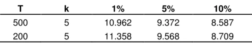
Table 5.1 Critical Values for the Sequential Maximum F Test

T k 1% 5% 10%

500 5 10.962 9.372 8.587 200 5 11.358 9.568 8.709

5.3 Results of Sequential Fmax Test

5.3.1 Testing the whole sample

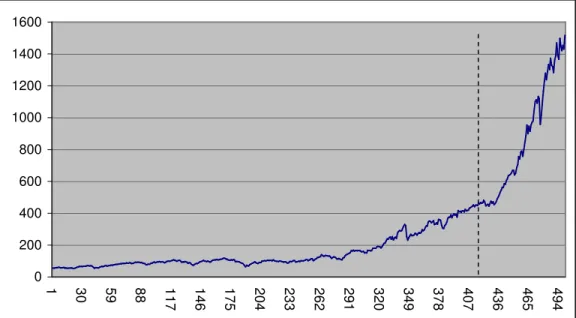
I apply the sequential maximum F test given in equation (4) to SP&500 monthly data. In the first part of the study, I test the complete sample. Results are given in Figure 5.1 and Figure 5.2.

Maximum F value is found as 15.638 and it’s larger than 10.962 which is the critical value of 1 percent significance level given in Table 5.1, null hypothesis is rejected at 1% significance level. Also break test found the break date on July 1993.

(41)

0 200 400 600 800 1000 1200 1400 1600 1 3 0 59 88 11 7 1 4 6 1 7 5 2 0 4 2 3 3 2 6 2 2 9 1 3 2 0 3 4 9 3 7 8 4 0 7 4 3 6 4 6 5 4 9 4

Figure 5.1 Stock prices with respect to months (dashed line mentions the break date) 0 2 4 6 8 10 12 14 16 18 1 3 1 61 91 12 1 1 5 1 1 8 1 2 1 1 2 4 1 2 7 1 3 0 1 3 3 1 3 6 1 3 9 1 4 2 1 4 5 1 4 8 1

Figure 5.2 F values with respect to months (dashed line mentions 1 percent significance level)

(42)

Visual inspection of Figure 5.1 shows two likely breaks in the data set at data points approximately 280 and 430 while the break point proposed by the test is at 415 between these two dates. Since the test used in this study is a single break test, its performance with multiple breaks is not known. When there is more than one break, as a characteristic of the test it finds the proposed single break point between these multi break points. There are multiple structural break tests that deal with this problem, but since they have so many problems in determining the break points and estimating the parameters, single break test is preferred in this empirical study. What we propose to deal with this problem is to separate the data set by using the break point found by the break test as a reference point. For this particular data set there seems to be two break points, and the proposed data point falls between these points. Dividing the sample into two at the proposed point might give single breaks in each part, which might increase the effectiveness of the test. Therefore when we apply the sequential F test, these smaller data sets separately we can get the correct result as there is only structural break in these sets.

One of the main problems about the test that I mentioned in the theoretical part of this study occurs again in the empirical section. Although the F test rejected the joint null hypothesis (nonstationarity, no break in mean and trend); we don’t know which part of this joint null hypothesis is rejected. Test may reject the nonstationarity or break in trend or break in mean or may be all of these three cases. We can’t determine which of these cases rejected by only looking the F values. However, we can supplement our results by examining the parameters and their t-statistics separately.

(43)

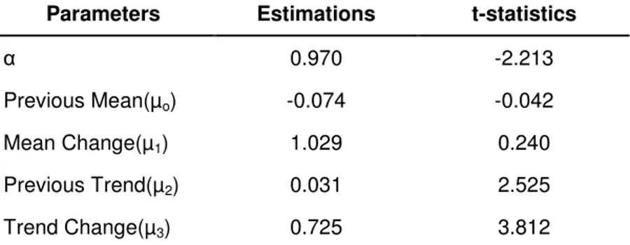
Table 5.2 Ordinary Least Square Estimation Results for the Sequential F Test

Parameters Estimations t-statistics

α 0.970 -2.213

Previous Mean(µo) -0.074 -0.042 Mean Change(µ1) 1.029 0.240 Previous Trend(µ2) 0.031 2.525 Trend Change(µ3) 0.725 3.812

Note: In t statistics, for mean and trend break no break case and for α unit root is taken as null hypothesis By looking over the results of the test in Table 5.2, we can see that mean change is insignificant since t statistic of mean change is smaller than the critical values for t distribution. Therefore we can’t reject that mean change is indifferent from 0. Thus we can conclude that there is not any significant mean change and rejection of null hypothesis is not because of mean break.

In addition to this, estimation of unit root parameter (α) is nearly 1. This can be an evidence for the unit root property in the stock market data. In addition, t statistic of this variable is -2.213 and its absolute value is smaller than the critical values in Dickey Fuller Distribution table. Therefore we can’t reject that α is one with respect to the t-statistics. Thus, t-statistics and estimation of parameters are supporting the unit root property and we can say that main reason under the rejection of the joint null hypotheses can’t be the rejection of the nonstationarity of the data set.

If we examine the trend change parameter, it is estimated as 0.725 and its t statistic is 3.812 as given in Table 5.2. Estimation of the parameter is much larger than the estimated previous trend (0.031) so we can say there can be a significant change in trend. Also t statistic is significant at 5 percent level with respect to the critical values given in Dickey Fuller table. Therefore, we can reject the no break case in trend with the

(44)

t-statistics. Thus, we can now say that real reason behind the rejection of the joint null hypothesis is trend break for the whole stock market data.

The formation of the whole stock price data resembles the third scenario, nonstationary case with only trend break. As it is noticed in theoretical part, results of the Monte Carlo simulations are quite good. Although small sample size problem is important, estimates of parameters are almost the same with the true values. Therefore, based on the simulations in the theoretical part, the test performs well for parameter estimation during the examination of the whole stock market data set.

The reliability of these results is still suspicious; however, because sequential break test used in this study is prepared for the single break, its results may not be correct for multiple breaks. So as I mentioned before, in order to tackle this problem, I divide the data set and test again. As mentioned before, one has to be aware of small sample size problems. For the whole data set since there are 500 observations there is not any small sample size problem, but if we separate the data set small sample becomes a relevant issue.

5.3.2 Division of the Data Set

As mentioned earlier in multiple break cases, single structural break test seems to find the break between the actual break points. Since in our stock market data there seems to be multiple break points, our single break test will detect the break between these two data points. Therefore, we can take the result of the single break test as a reference point for separation. Break point is found at data point of 415 while testing the whole data. By taking the first data set just after the 415 as 435, we can be on the safe

(45)

side to capture the single break between 0 and 435. Also by taking data set as large as possible we protect ourselves from the effects of small sample size problems. For the second data set again main problem is number of observations. If we take it between 415 and 500, sample size will be only 75 and there will large effects of small sample size. In order to avoid from the effects of the sample size and to cover only one break point sample size is chosen as 250 and the second data set is determined between the points of 250 and 500.

5.3.3 Testing Data set 1

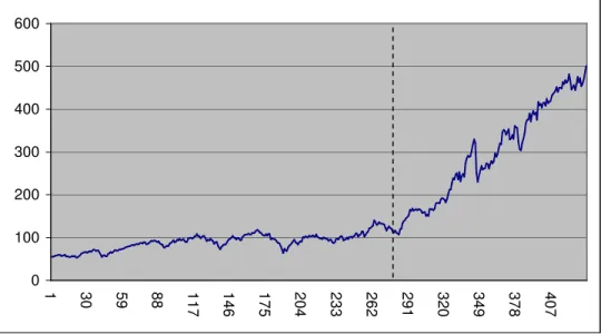
Data set 1 is determined as the set covering the data points 0 to 435 in the whole sample of 500 data points. After applying the sequential maximum F test given in equation (4.2) to the data set 1 which covers the monthly data of SP&500 from the year 1959 to 1994.

Maximum F value is found as 16.779 and it’s larger than 10.962 which is the critical value of 1 percent significance level given in Table 5.1, null hypothesis is rejected at 1% significance level. Also break test found the proposed break date on June 1982. The break date can also be seen in the Figure 5.3, which is marked with the dashed line. The main problem at this point is that although the maximum F values reject the joint null hypothesis (nonstationarity, no break in mean and trend); we don’t know which part of the joint null hypothesis is rejected. If we examine the Figure 5.3, at the break date we can notice the the change in the slope of the stock market data. However, until we examine the t-statistics and estimations of parameters we can’t say anything about the reason behind the structural break at the break point.

(46)

0 100 200 300 400 500 600 1 3₀ 5₉ 8₈ 1₁ 7 1 4 6 1 7 5 2 0 4 2 3 3 2 6 2 2 9 1 3 2 0 3 4 9 3 7 8 4 0 7

Figure 5.3 Stock prices with respect to months (dashed line mentions the break date) 0 2 4 6 8 10 12 14 16 18 3 2 5 84 70 92 11₄ 13₆ ₇15 17₉ 20₁ 22₃ ₄42 26₆ 28₈ 31₀ ₁33 35₃ 37₅ 39₇ 41₈

Figure 5.4 F values with respect to months (dashed line mentions 1 percent significance level)

(47)

Table 5.3 Ordinary Least Square Estimation Results for Data Set 1

Parameters Estimations t-statistics

α 0.807 -6.581

Previous Mean(µo) 12.919 6.469 Mean Change(µ1) 1.176 0.699 Previous Trend(µ2) 0.034 3.977 Trend Change(µ3) 0.440 6.508

Note: In t statistics, for mean and trend break no break case and for α unit root is taken as null hypothesis Estimations and related t-statistics are given in Table 5.3. By examining the results of the test in Table 5.3, we can observe that mean change is insignificant. So, we can’t reject that mean change is different from 0. Thus, we can conclude that there is not any significant mean change and rejection of null hypothesis is not due to a mean break. In addition to this, estimation of unit root parameter (α) is estimated as 0.807 and since this is not close to 1 it can not support unit root property. T-statistics of α is -6.581 and in absolute values it is larger than the critical value of -3.980 for 1 percent significance level as given in Dickey Fuller Distribution table. Therefore, we can reject that α is one and we can say that our data set is stationary with respect to the t-statistics and estimations. Thus, t-statistics and estimation of parameters are supporting the stationarity; we can say that one possible reason behind the rejection of the joint null hypotheses can be the stationarity of the data set.

The trend change parameter is estimated as 0.440 and its t-statistics is 6.508 as given in Table 5.3. Estimated change in trend is much larger than the estimated previous trend (0.034), so we can say there is a significant change in trend. Also t-statistics is significant at 1 percent level since tstatistics 6.508 is larger than the absolute value of -3.980 which is given in Dickey Fuller table. Therefore, we can reject the no break case