CO-EXPRESSION PAIRS AND MODULES (CoEX-PM): A SHINY
APPLICATION AND AN EXAMPLE CASE STUDY ON
CHROMOGRANINS
A THESIS SUBMITTED TO
THE GRADUATE SCHOOL OF ENGINEERING AND SCIENCE
OF BILKENT UNIVERSITY
IN PARTIAL FULLFILLMENT OF THE REQUIREMENTS FOR
THE DEGREE OF
MASTER OF SCIENCE
IN
NEUROSCIENCE
By
Tuğberk Kaya
September 2018
ii
CO-EXPRESSION PAIRS AND MODULES (CoEX-PM): A SHINY APPLICATION AND AN EXAMPLE CASE STUDY ON CHROMOGRANINS
By Tuğberk Kaya September 2018
We certify that we have read this thesis and that in our opinion it is fully adequate, in scope and in quality, as a thesis for the degree of Master of Science.
Özlen Konu Karakayalı (Advisor)
Michelle Marie Adams
Aybar Can Acar
Approved for the Graduate School of Engineering and Science:
Ezhan Karasan
iii
ABSTRACT
CO-EXPRESSION PAIRS AND MODULES (CoEX-PM): A SHINY
APPLICATION AND AN EXAMPLE CASE STUDY ON
CHROMOGRANINS
Tuğberk Kaya M.Sc. in Neuroscience Advisor: Özlen Konu Karakayalı
September 2018
Gene expression signatures have been proved to be effective biomarkers of tumorigenesis and metastasis especially when alternative methods are inconvenient or ineffective. Nevertheless, handling very large datasets obtained via high-throughput protocols to extract gene expression signatures may prove challenging. A great number of software packages that facilitate such analyses have been written in R programming language are publicly available and free. However, the relatively steep learning curve that is required to use R proficiently prevents the utilization of these packages. I have developed the Shiny application Co-expression Modules and Pairs
(CoEX-PM) using R programming language and the R package shiny. The CoEX-PM
application handles human Affymetrix microarray data and enables users to generate pairwise correlation plots, conduct meta-correlation analysis with user-selected GEO datasets along with co-expression module generation by WGCNA program for genes of interest. The CoEX-PM application provides the user with a GUI, therefore, does not require any coding knowledge to perform the analyses.
Pheochromocytoma (PCC) and neuroblastoma (NB) are neural-crest derived tumors, common in adults and children, respectively and are both associated with high-rate of morbidity and
mortality. In addition, both tumor types display neuroendocrine tumor (NET) characteristics. Chromogranin A (CgA) has been linked with NETs as a moderately sensitive and non-specific tumor marker. The chromogranin family consists of up to seven members, three of which are
iv
chromogranin (CgA), chromogranin B (CgB) and secretogranin II (SgII) or occasionally named as chromogranin C (CgC). However, it is not known whether chromogranin/secretogranin family members are differentially expressed in PCC and NB. Here, I investigate the degree of co-expression in gene networks by analyzing gene co-expression signatures of the
chromogranin/secretogranin paralogous gene family using CoEX-PM application on neuroendocrine tumor datasets. The findings indicate presence of concise and highly
v
ÖZET
KO-EKSPRESYON ÇİFTLERİ VE MODÜLLERİ (CoEX-PM): BİR
SHINY APLİKASYONU VE KROMOGRANİNLER ÜZERİNDE BİR
İNCELEME
Tuğberk Kaya Nörobilim, Yüksek Lisans Tez Danışmanı: Özlen Konu Karakayalı
Eylül 2018
Gen ekspresyon profillerinin, özellikle alternatif metodlar yetersiz ve etkisiz kaldığında, etkin tümörijenez ve metastaz bio-belirteçleri oldukları kanıtlanmıştır. Bununla birlikte, yüksek verimli protokoller aracılığıyla elde edilen büyük veri kümelerini analiz ederek gen ekspresyon profilleri bulmaya çalışmak zorlu olabilir. R programlama dilinde bu tip analizleri kolaylaştıran çok sayıda yazılım paketi ücretsiz kullanıma açık şekilde yer almaktadır. Fakat, R'yi etkili bir şekilde kullanmak için gerekli olan nispeten sarp öğrenme eğrisi, bu paketlerin kullanılmasını kimi zaman engellemektedir. Bu tez kapsamında R programlama dili ve shiny paketini
kullanarak CoEX-PM aplikasyonunu geliştirdim. CoEX-PM uygulaması, insan Affymetrix mikrodizi verilerini kullanır ve kullanıcıların çift yönlü korelasyon grafikleri oluşturmasına, kullanıcı tarafından seçilen GEO veri kümeleriyle meta-korelasyon analizi gerçekleştirmesine ve ilgili genler için WGCNA programı ile birlikte ko-ekpresyon gen modülleri oluşturmasına olanak tanır. CoEX-PM tüm bu analizleri gerçekleştirmesi için kullanıcıya bir arayüz sağlar, bu nedenle herhangi bir kodlama bilgisi veya tecrübesi gerektirmemektedir.
Pheochromocytoma (PCC) ve nöroblastoma (NB), sırasıyla yetişkinlerde ve çocuklarda sık görülen nöral-krest kaynaklı tümörlerdir ve her ikisi de yüksek oranda morbidite ve mortalite ile ilişkilidir. Ek olarak, her iki tümör tipi de nöroendokrin tümör (NET) özelliklerini gösterir. Kromogranin A (CgA), orta derecede hassas ve spesifik olmayan bir nöroendokrin tümör markörü olarak rapor edilmiştir. Kromogranin ailesinin 7 üyesi vardır, bunlardan üçü
vi
kromogranin (CgA), kromogranin B (CgB) ve sekretogranin II (SgII) veya kimi zaman kromogranin C (CgC) olarak adlandırılır. Kromogranin / secretogranin aile üyelerinin PCC ve NB'de farklı ko-ekspresyon şekilleri gösterip göstermedikleri bilinmemektedir. Bu tezde, nöroendokrin tümör veri kümeleri üzerinde CoEX-PM uygulaması kullanılarak kromogranin / secretogranin paralog gen ailesinin gen ekspresyon imzaları analiz edilmiş, gen ağlarındaki ko-ekspresyon derecesi araştırılmıştır. Bulgular, kromogranin ko-ekspresyon seviyesi ile bağlantılı, PCC ve NB'de özlü ve yüksek düzeyde birlikte ifade edilen fonksiyonel bileşenlerin varlığını göstermektedir.
vii
Acknowledgements
I acknowledge that I was financially supported in the form of monthly stipends by the Neuroscience Department affiliated with the Graduate School of Engineering and Science, Bilkent University.
I would like to express my deepest gratitude to my thesis advisor Dr. Özlen Konu for always supporting me even through the darkest times, pointing at the right direction and keeping me on track. I thank Drs. Michelle M. Adams and Aybar C. Acar for being members of my thesis committee and helpful comments they provided. I also thank Dr. Huma Shehwana for sharing her R codes when needed and Alperen Taciroğlu for valuable discussions on shiny applications. I thank all the members of Konu lab for their constant positivity and willingness to help each other without hesitation. Lastly, I’d like to thank my friends and family who are the ones that make it all worth it.
viii
Contents
1.
Introduction ... 1
Web tools using Shiny for gene expression analysis ... 1
Neuroendocrine tumors and their classification ... 2
Incidence and prevalence of NETs ... 3
Pheochromocytomas/Paragangliomas ... 4
Neuroblastoma ... 4
Microarray Technology ... 5
Meta-Analysis ... 6
Previous microarray studies focusing on Pheochromocytoma ... 8
Neuroendocrine Tumor (NET) Biomarkers ... 9
Biomarker limitations and issues ... 10
Chromogranins: structure and function and evolution ... 12
2. Aims ... 13
3. Methods ... 15
3.1. Data Acquisition and Normalization ... 15
3.2. Shiny Application Design ... 16
3.2.1. Tab 1: Pairwise correlation analysis. ... 17
3.2.2. Tab 2: Meta-analysis Tab ... 18
Metacor package ... 18
3.2.3. Tab 3: WGCNA Tab ... 18
4.
Results ... 20
4.1. COEX-PM Application ... 20
4.1.1 Gene-Correlation Tab ... 20
4.1.2. Meta-correlation Tab ... 24
4.1.3. WGCNA Tab ... 25
4.2. Case-study: Chromogranins in NETs ... 29
ix
4.2.2. Meta-correlation of CHGA and CHGB across transcriptome ... 39
4.2.3 Chromogranin and Secretogranin Co-expression modules using WGCNA Tab ... 61
Conclusions and Discussion ... 79
Future Prospects ... 85
x
Table of Figures
Figure 1:The screenshot of Sample Clustering part of the Two Gene Correlation Tab. ... 21 Figure 2: The screenshot of Plot part of the Two Gene Correlation Tab. ... 23 Figure 3: The screenshot of Meta-correlation Tab ... 24 Figure 4: The screenshot of WCGNA Tab: Limma Differential Gene Expression Analysis – Phenodata table. ... 25 Figure 5: The screenshot of WCGNA Tab: Limma Differential Gene Expression Analysis – limma table... 26 Figure 6: WGCNA Tab: Sample Clustering and Power Analysis – Sample clustering scheme ... 27 Figure 7: Network topology analysis plots for various soft-thresholding powers. ... 28 Figure 8: WGCNA Tab: Module Construction – Module dendrogram of genes, each color
represents a different module, grey color is reserved for genes that are not a member of any module... 28 Figure 9: CHGA-CHGB correlation plots for nine distinct datasets. GSE67066, GSE2841 – PCC; GSE13136, GSE16476, GSE16237, GSE12460 – neuroblastoma; GSE39612 – Merkel cell carcinoma; GSE35679 – lung carcinoid, GSE12667 – lung adenocarcinoma. ... 30 Figure 10: Correlation plots of chromogranins of interest (CHGA-CHGB) with secretogranin genes of interest (SCG2-3-5) for the GSE67066 dataset (PCC, pheochromocytoma). The color gradient implies the expression level. ... 31 Figure 11: Correlation plots of chromogranin of interest (CHGA-CHGB) with secretogranin genes of interest (SCG2-3-5) for the GSE2841 dataset. The color gradient implies the expression level. GSE2841 contains 76 pheochromocytoma samples of various genetic origin. ... 32 Figure 12: Correlation plots of chromogranin of interest (CHGA-CHGB) with secretogranin genes of interest (SCG2-3-5) for the GSE16476 dataset. The color gradient implies the
expression level. GSE16476 contains 88 human neuroblastoma samples. ... 33 Figure 13: Correlation plots of chromogranin of interest (CHGA-CHGB) with secretogranin genes of interest (SCG2-3-5) for the GSE13136 dataset. The color gradient implies the
expression level. GSE13136 contains 30 primary neuroblastoma samples. ... 34 Figure 14: Correlation plots of chromogranin of interest (CHGA-CHGB) with secretogranin genes of interest (SCG2-3-5) for the GSE12460 dataset. The color gradient implies the
expression level. GSE12460 contains 64 neuroblastic tumors (mainly neuroblastoma). ... 35 Figure 15: Correlation plots of chromogranin of interest (CHGA-CHGB) with secretogranin genes of interest (SCG2-3-5) for the GSE35679 dataset. The color gradient implies the
expression level. GSE35679 contains 13 primary lung carcinoid samples. ... 36 Figure 16: Correlation plots of chromogranin of interest (CHGA-CHGB) with secretogranin genes of interest (SCG2-3-5) for the GSE12667 dataset. The color gradient implies the
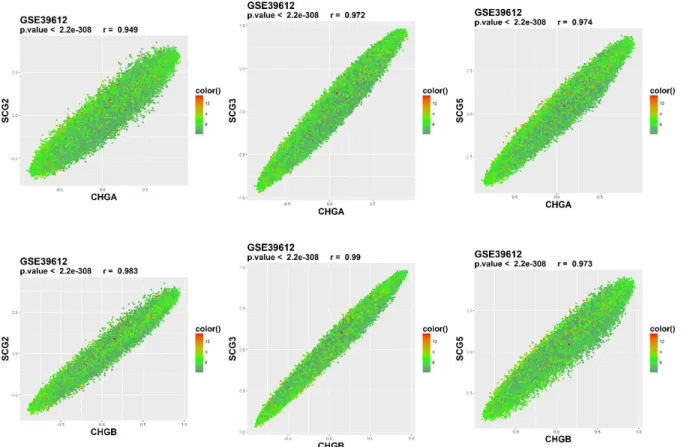
expression level. GSE12667 contains 75 lung adenocarcinoma samples... 37 Figure 17:Correlation plots of chromogranin of interest (CHGA-CHGB) with secretogranin genes of interest (SCG2-3-5) for the GSE39612 dataset. The color gradient implies the
expression level. ... 38 Figure 18: Histogram of r.mean values for CHGA (Left) and CHGB (right). The r.mean values was generated a result of the meta-correlation analysis using the GSE67066 and GSE2841 (PCC) datasets. ... 39 Figure 19:Correlation plot of the r.mean values for CHGA and CHGB. The r.mean values was generated a result of the meta-correlation analysis using the GSE67066 and GSE2841 (PCC)
xi
datasets. The color gradient represents the chromogranin divergence (chga - chgb). ... 40 Figure 20: Protein-Protein interaction network of genes selected after meta-correlation analysis of GSE16476_GSE12460_GSE13136_GSE73537_GSE16237 (neuroblastoma) for the CHGB gene. Genes with r.mean>0.55 and p value < 0.003 were selected for the STRING mapping. ... 43 Figure 21: Functional enrichment results for the selected genes mentioned in Figure 20. ... 44 Figure 22: Protein-Protein interaction network of genes selected after meta-correlation analysis of GSE16476_GSE12460_GSE13136_GSE73537_GSE16237 (neuroblastoma) for the CHGA gene. Genes with r.mean>0.48 were selected for the STRING mapping . ... 45 Figure 23: The functional annotation of CHGA PPI network in Figure 22. ... 46 Figure 24: Protein-Protein interaction network of genes selected after meta-correlation analysis of GSE16476_GSE12460_GSE13136_GSE73537_GSE16237 (neuroblastoma) for the SCG2 gene. Genes with r.mean>0.65 were selected for the STRING mapping ... 47 Figure 25: Functional annotation of Protein-Protein interaction network in Figure 24. ... 48 Figure 26: Protein-Protein interaction network of genes selected after meta-correlation analysis of GSE16476_GSE12460_GSE13136_GSE73537_GSE16237 (neuroblastoma) for the SCG3 gene. Genes with r.mean>0.6 were selected for the STRING mapping. ... 49 Figure 27: Functional annotation of PPI network in Figure 26. ... 50 Figure 28: PPI network of genes selected after meta-correlation analysis of GSE67066_GSE2841 (PCC) for the CHGA gene. Genes with r.mean>0.6 were selected for the STRING mapping .... 51 Figure 29: Functional annotation of PPI network in Figure 28. ... 52 Figure 30: PPI network of genes selected after meta-correlation analysis of GSE67066_GSE2841 (PCC) for the CHGB gene. Genes with r.mean>0.6 were selected for the STRING mapping. ... 53 Figure 31: Functional annotation of PPI network in Figure 30. ... 54 Figure 32: PPI network of genes selected after meta-correlation analysis of GSE67066_GSE2841 (PCC) for the SCG2 gene. Genes with r.mean>0.65 were selected for the STRING mapping. ... 55 Figure 33: Functional annotation of PPI network in Figure 32. ... 56 Figure 34: PPI network of genes selected after meta-correlation analysis of GSE67066_GSE2841 (PCC) for the SCG3 gene. Genes with r.mean>0.58 were selected for the STRING mapping. ... 57 Figure 35: Functional annotation of PPI network in Figure 34. ... 58 Figure 36: PPI network of genes selected after meta-correlation analysis of GSE67066_GSE2841 (PCC) for the SCG5 gene. Genes with r.mean>0.65 were selected for the STRING mapping. ... 59 Figure 37: Functional annotation of PPI network in Figure 36. ... 60 Figure 38: Sample clustering for GSE67066 with a cut-off line at 140. ... 61 Figure 39: Network topology analysis for filtered GSE67066. ... 62 Figure 40: Clustering dendrogram of probes, with dissimilarity based on topological overlap. Module colors are shown for their assigned probes... 64 Figure 41: Module-gene associations, first part. Rows correspond to module eigengenes,
columns to genes of interest. Each cell displays the corresponding correlation and p-value. Color coding is established by correlation according to the legend. ... 65 Figure 42: Module-gene associations, second part. Rows correspond to module eigengenes, columns to genes of interest. Each cell displays the corresponding correlation and p-value. Color coding is established by correlation according to the legend. ... 66 Figure 43: Scatterplot of Gene Significance (GS) for SCG2 and CHGA for Module Membership (MM) in the black and red modules, respectively. ... 68 Figure 44: Hierarchical clustering dendrogram of the eigengenes and the genes of interest. ... 69 Figure 45: The heatmap of eigengene adjacency with gene of interests added. ... 69
xii
Figure 46: PPI network of black module genes with top 200 Gene Significance. ... 72
Figure 47: PPI network of red module genes with top 200 GS. ... 74
Figure 48: PPI network of salmon module genes. ... 75
xiii
List of Tables
Table 1: The datasets that were acquired from the GEO database and used in further analyses. . 16 Table 2 : Functional annotation table for genes with high chga-chgb r.mean ... 41 Table 3: Functional annotation table for genes with low chga-chgb r.mean... 41 Table 4: Most correlated MEs for each gene of interest. ... 67
1
1. Introduction
Accumulation of massive amounts of high-throughput data in publicly open repositories such as Gene Expression Omnibus (GEO) and ArrayExpress have been crucial in enabling researchers to access and share data online for free. Over the last decades, microarray studies have provided great insight about the disease state with regards to tumorigenesis and metastasis; microarrays also provide researchers with ways to determine significant patterns of gene
expression that characterize the tumor state. However, there is still a need to integrate different data types to analyze co-expression of pairs of genes from high throughput expression datasets effectively yet tools that contain graphical user interfaces (GUI) on the WWW are scarce.
The characterization of elements underlying neuroendocrine tumors are of particular interest for this thesis. The origin of neuroendocrine tumors vary greatly and so does their physiological features, which make their prognosis and intervention dramatically difficult. Gene expression signatures have proved to be effective biomarkers of tumorigenesis and metastasis when other methods of diagnosis are inadequate. On the other hand, analyzing and manipulation of very large datasets obtained via high-throughput protocols poses multiple challenges.
Nevertheless, a great number of packages in R programming language have been written by expert programmers to assist researchers in handling very large biological datasets. However, there is a steep learning curve to overcome to use R effectively and this might make it difficult to utilize these valuable packages. The R package Shiny is a web application framework for R and lets the users to develop applications that conduct simple or complex analyses written in R.
Web tools using Shiny for gene expression analysis
There is a need in the literature for efficient tools that conduct gene expression analysis as well as bypass the coding process and convert the process to a customizable interface. There have been multiple studies addressing this problem; using Shiny to develop applications that facilitate high-throughput expression data analysis.
2
multiple GEO datasets. This application enables the parallel analysis of GEO datasets. It retrieves relevant datasets using the selected organism and an optional search term. For the differential gene expression part, a custom list of genes or a KEGG pathway is selected. The results consist of a list of most significant genes and a list of studies with the most number of significant genes.
Another Shiny application that handles GEO datasets is the shinyGEO 2 application.
When an accession number and platform name is entered, a table is obtained from the GEO, displaying a summary of the clinical data for the dataset. It is possible to conduct differential expression analysis or, if relevant to the dataset, survival analysis by inputting a probe ID of interest and a phenodata column to determine the groups for comparison. The output is the visualization of the log2 expression of the selected gene.
Differential gene expression analysis is not the only method implemented in Shiny applications. NAP: The network analysis profiler 3 is an online tool that automates network
profiling and topology comparison. Methylation plotter 4 enables dynamic visualization of
user-provided DNA methylation data. In the literature, there are various operations built-in Shiny applications, ranging from categorization to interactive plotting of expression data.
Neuroendocrine tumors and their classification
Neuroendocrine tumors (NETs) are a diverse group of neoplasms that involve various organs and display diverse biological characteristics. Due to the diffuse nature of the
neuroendocrine system, NETs vary greatly in their tissue of origin. Nonetheless, they share common pathological features regardless of anatomical site thus have been primarily classified accordingly and further specified with regards to tumor differentiation, hormones or amines secreted, and tumor grade and stage 5.
In some instances, excessive hormone secretion due to neuroendocrine nature of the tumor leads to clinical symptoms and syndromes; this phenomenon is referred to as tumor functionality and has been used in the literature for NETs secreting active bio-compounds 6.
3
types of NETs, the biological tendencies of a neuroendocrine tumor is mainly influenced by how far the tumor has progressed in terms of stage and grade. Thus, the diagnosis process for both non-functional and functional NETs that originated from the same organ is identical 5.
In general, NETs are slow-growing tumors. They can originate in various parts of the human body but they are more commonly seen in pancreas, GI tract, lung and some other organs that display endocrine characteristics. As mentioned earlier, it has been discovered that NETs are able to synthesize and secrete certain products; the peptides or amines secreted by the NETs often lead to pathological symptoms and are utilized as tumor markers 7.
Incidence and prevalence of NETs
NETs are seen in every five in a thousand of all cancers 8. The incidence rate is about two
in a million. This number has slowly increased from 19 to 52/100,0000 people per year
throughout the last 30 years 910. Among the tumors of the same organ, incidence of NETs have a
higher rate of increase 11. NETs increase with age and peak between 50-70 years. Modernization
of the diagnostic tools and accumulation of empirical data about the disease are implied to be the major factors driving the increase for incidence rate of NETs 12. Because NETs progress slowly,
their incidence correlate positively with their prevalence which has been estimated to be 35:100,000 a year.
NETs are observed with some differences but mostly similarities among different demographic groups. Incidence rates of NETs between men and women are very similar in the U.S. 13, however, there are exceptions to the rule, NETs that arise from rectal sites have a higher
rate of occurrence in men than women 14. Pancreatic NETs and the small intestinal NETs have
also slightly higher incidence rates in males but low-grade NETs and lung NETs appear with a higher rate of incidence in women 15.
4
Pheochromocytomas/Paragangliomas
Pheochromocytomas (PCCs) are rare types of tumors arising in neural crest tissue. When located at extra-adrenal tissue, they are designated as paragangliomas (PGLs). PCCs and PGLs share a common site of origin; they are both derived from neuro-ectoderm. In addition, PCCs are more correctly referred to as intra-adrenal paragangliomas 5. Pheochromocytomas and
paragangliomas show very similar fundamental histological characteristics. Parasympathetic PGLs more often arise from the head and neck tissues whereas sympathetic PGLs could be found in either adrenal medulla (namely PCCs) or at the thoracic, abdominal or pelvic area 16.
.
Neuroblastoma
Neuroblastoma is an early (childhood or embryonal) tumor that arises from the autonomic nervous system, mainly the peripheral sympathetic nervous system. Therefore, the tumor is derived from the neural-crest tissues while its site of origin is a precursor cell that is still developing 17. Since it is a disease of developing tissues, the affected demographics consist of
mostly children as young as 17 months 18. Typically, sympathetic nervous tissue is the site of
origin for these tumors, arising from the paraspinal ganglia and adrenal medulla; the tumors result in mass lesions that could be observed in chest, abdomen, pelvis and neck area. The clinical manifestation of the disease is highly prone to variability. The disease is highly common in very young children, in fact it is the most common cancer type that manifests during the first year of life 19.
Throughout many decades of clinical evidence and research, it has been noted that neuroblastomas are associated with unpredictable and dramatic clinical symptoms 20. In parallel
with its unusual nature, neuroblastoma is the leading cause for mortality among the childhood cancers, but at the same time, it is one of the cancers that has received significant improvement in survival rates in recent decades 21 Data collected by the Surveillance, Epidemiology, and End
1999-5
2005 increased from 52% to 74%, respectively 20. However, this improvement is mainly due to
better outcome in patients with more benign tumors; the survival or cure rates among the
children with aggressive neuroblastoma have seen only a moderate increase, despite the dramatic improvements in therapy technologies and methods 22.
Neuroblastoma has been widely considered to be an aggressive and abnormal representation of the developing sympathetic nervous system tissue, however, until the last decade, there has been a lack of knowledge in terms of the genetic basis of the condition. Similar to other cancer types, a group of cases has been identified to exhibit autosomal dominant
inheritance. The results of the study conducted by Mosse et al. showed that in most cases of hereditary neuroblastoma, activation of mutations are observed in the tyrosine kinase domain of anaplastic lymphoma kinase (ALK) 23. In addition, loss-of-function mutations in PHOX2B gene
is present in children with sporadic or familial neuroblastoma who are also diagnosed with Hirschsprung’s disease, congenital central hypoventilation syndrome, or both 24. Therefore, if a
patient has a family history of neuroblastoma or other clinical complications with a high-risk mutation, genetic screening for mutations in both of these risk genes, ALK and PHOX2B, should be considered. In addition, a recent study has implicated chromogranins in blood of
neuroblastoma patients with prognosis of the disease suggesting further research into chromogranin family is needed in this cancer type 25.
Microarray Technology
For a long time, molecular biologists could analyze one of few genes at a time since the techniques depended on methods using nucleic acid probes (in situ hybridization, Norther blotting, etc.) or antibodies (Western blotting, etc.). The emergence of genomic information and advancement of array-based profiling technologies have made it possible to obtain information about the state of thousands of genes in a single assay. The basis for the microarray concept is as follows; RNA isolation is performed using samples of interest to process the isolated RNA and produce the target sequence which is being tested in terms of abundance or identity. Next, the target binds to the probes that are in a pre-determined formation on the array and consist of sequences that correspond to certain genes. The hybridization taking place between the target
6
and the tethered probe enables a measurement by quantifying the hybridization affinity for each target. This quantitative data characteristic is obtained via software and processed through many pipelines in order to extract biological information 26. Microarrays have been primarily used to
measure gene expression levels.
An array is sensitive only to the sequences it was design to detect. In other words, if the solution that is to be hybridized contains sequences with no complementary sequence on the platform matrix, it is not possible to detect those sequences using an array platform with that particular set of probes. As far as gene expression analysis purposes are concerned, this basically implies that only genes who are members of previously annotated reference genomes will be present on the array. This can prove especially problematic for genomes with high variability such as bacteria 27. On the other hand, one critical advantage of microarray datasets is their
widespread and frequent usage allowing conductance of meta-analysis to obtain reliable conclusions based on transcriptomics in different species.
Meta-Analysis
Due to the advancement of high-throughput omics data generation technologies and their increasing availability, researchers from almost every medical field are able to utilize these methods. Nevertheless, robust data analysis methods are required to be able to wholly interpret the biological meaning in the massive data. The availability of the microarray technology
contributed to the cumulative abundance of transcriptomic data as well as RNA-seq experiments which have been especially significant in the last decade. In order to collect, store and share the growing body of large data publicly, online repositories Gene Expression Omnibus (GEO)28and
ArrayExpress 29, were established and proved tremendously useful in terms of availability and
accessibility of raw data.
More often than not, multiple transcriptomic studies that focus on a similar pathological state are available although, even more often, it is the case that each study is based on a small number of samples, therefore lacking significance for their findings. If the data used in each study were merged, the statistical power of the analysis and the significance of the findings would increase 30. Nevertheless, it is problematic to compare heterogeneous datasets directly
7
due to inherent complications in biological and experimental parameters 31.
Meta-analysis, which is composed of statistical tools and approaches to merge data from multiple studies is a practical solution to overcome the abovementioned challenges. Overall, meta-analysis is an invaluable tool for researchers who are interested in investigating existing datasets to identify potential biomarkers and pathways. Arguably, one of the biggest problems of microarray studies is that since there are thousands of probes, each representing a different hypothesis with relatively small number of samples, thus the statistical power of the analysis dramatically drops. Accepting a very conventional positive rate of 0.05 in array platform with over 50,000 probes would mean over 2500 genes are seen as a differential element due to mere chance only 32. Merging the data from multiple studies provides more robust results so that the
false positively significant genes will not be present whereas the true positives can still be observed.
In addition to random noise, another factor that contributes to false discovery is biological and experimental differences in the study design 30. There is no doubt that some
variation in gene expression levels identified by different studies are the result of true biological variation in samples. However, distinct experimental parameters such as use of different media at different concentrations could alter the results even when using identical cell lines. This type of experimental variation holds “true” in the context of those particular experimental conditions but still will not be reproducible in other studies with slightly altered conditions 30. Meta-analysis
helps prevent such experimental factors and presence of outliers from affecting the results and helps unmask the true and consistent significant findings.
While conducting a meta-analysis, it is required to control for additional systematic biases or effects other than biological and experimental factors – sometimes referred to as “lab effect” to emphasize the potential variability stemming from conditions in different laboratories – such as using data from different platforms (platform-effect) and even using samples from various species (species-effect) 33. Comparison or integration of data across platforms requires an
extra step. Due to the many-to-many relationship between genes and probes, in varying platforms the same gene may map to a different set of probes, therefore a common set of
8
identifiers should be constructed when mapping across platforms. 34. A robust cross-species
analysis is not among the purposes of this article, thus, no further details will be explained on the topic other than that an accurate knowledge of orthology is required and HomoloGene in NCBI and the Inparanoid 35 eukaryotic ortholog databases could be most useful 36.
Previous microarray studies focusing on Pheochromocytoma
There is a number of studies investigating the landscape of transcription profiling in PCC as well as NB. In this section, studies of significance to this article will be explained in brief fashion in terms of their methodology, hypotheses and findings. In addition, raw microarray data are available for almost all of the following studies and, those available, have been utilized for the purposes of this thesis as part of the datasets used for the meta-analysis (see methods for details).
In the study conducted by Dahia et al. 37,the researchers showed that there was a common
function shared by three genes thought to be responsible for hereditary PCCs. The authors of the study performed comparative analysis of expression profiling of 76 PCCs and PGLs with a variety of mutations that are representatives of distinct PCC syndromes, sporadic tumors and familial tumors without an identifiable mutation.
Until 2005, the year Dahlia et al. published their results, six independent genes were identified as inherited or sporadic mutation sites: RET, VHL, NF1 and subunits B, C and D of succinate dehydrogenase (SDH). To investigate the molecular interactions between the pathways that these aforementioned genes facilitate, Dahlia et al. conducted a microarray experiment using a large number of PCC samples 37. The results showed that, proteins encoded by specifically
VHL, SDHB and SDHD were important for the function of the transcription factor,
hypoxia-inducible factor 1 subunit alpha (HIF1) playing a facilitative role in adapting cells to low levels of oxygen or hypoxia. VHL has been linked to von Hippel-Lindau disease (VHL), the disease it is named after. VHL is an inherited disorder that makes individuals more susceptible to PCCs. It was reported in earlier studies that the absence of VHL leads to accumulation HIF1, and the lack of HIF1 degradation mimic a state of hypoxia 38.
9
Neuroendocrine Tumor (NET) Biomarkers
A fundamental and thorough knowledge of the nature of neoplasia structure is required to make further advancements in NET medical care 39. Nevertheless, another crucial unmet
requirement to investigate this class of tumors is the lack of robust biomarkers with proven statistical significance and biological convenience 40. Even with the diverse spectrum of
advancing technologies that contribute to modern medicine and therapeutic tools, detection of a disease state in the very early stages remains crucial. In addition, multi-utility tools that are able to track therapeutic efficacy and assess prognosis are needed to reveal robust biomarkers 41.
Single-analyte biomarkers have proved useful in the identification of distinct features of different disease states. The amount of information that single-analytes convey is not
comprehensive enough, failing to explain the diverse nature of NETs 41. It is required to acquire
and accumulate large omics datasets with a wide range of samples to create an understanding of NET diseases. Therefore, single-analyte measurements will become less reliable and the research paradigm is likely to shift towards the use of more comprehensive biomarkers such as multi-analytes. This turn of events represents an innovative step in establishing a system of
personalized medicine with the accumulation of multi-dimensional biological data. Similarly, using blood samples to acquire biological information compared to biopsy will enhance the robustness of the information and help avoid the potential risk factors involved in such invasive protocols 41.
Advancements in discovery-based approaches, such as microarray expression studies and proteomic approaches using mass spectrometry, have been critical in the identification of a number of candidate cancer biomarkers 42. The advent of microarray-based profiling along with
its rising availability has tremendously boosted the power to categorize cancers, notably breast tumors 43. But beyond the improvements on classification, these advances could be utilized for
solving fundamental problems in classification, such as presence of metastasis. A problem that often arises in clinical classification of metastatic tumors is determining the primary site of tumor origin. This problem, for example, could be solved by using classification techniques based on
10
gene expression signatures to predict the origin of the metastatic lesion based on its highest similarity to a tissue type. Accordingly, gene expression can provide more precise and extensive information about a tumor than histology could provide 42.
Scientific consensus on the validation of single-analyte biomarkers, for diagnosis and prognosis of NET, have shifted towards utilization of multi-analyte biomarkers based on the idea that a single-analyte test cannot account for the multidimensional pathophysiology of a
condition. In addition, the growing body of interdisciplinary research has contributed greatly to developing multi-analyte biomarkers by providing the necessary statistical power to analyze multi-variable complexes. NETs require secretion of neuroendocrine factors from vesicles and are associated with chromogranins 44. Accordingly, the multivariate nature of chromogranin
assemblies and the degree of divergence in these assemblies in between different cancers could be valuable to discover in the current biomarker field. However, there is no comprehensive study in the literature on this for PCCs and NBs or any other NETs. CgA, the protein encoded by the
CHGA gene is the major non-specific marker of NETs 44. CgA levels correlate with malignancy
and it has been reported that non-elevated levels of CgA could be an evidence leading to exclusion of PCC among the candidate for the disease state 45.
Biomarker limitations and issues
Ideally, a biomarker should be exclusively related to and representative of the particular disease state of interest while exhibiting an observable signal without background noise from irrelevant disease states. Gene expression profiling has been seen as a tool with great utility but its shortcomings should be evaluated as well. Although a vast number of genes, in scales of thousands, are detected to be highly expressed in malignant tissue compared to benign, a rather limited number of proteins or transcripts have been detected to have elevated states in tumor pathology 46. This problem does not necessarily make gene expression profiling a less significant
tool or obsolete but it shows that enhancements are needed. Development of analytically robust algorithms based on advanced statistics to detect abnormalities that are capable of discriminating among specific types of neoplasia as well as providing information about its pathological
11
To some extent, economic constraints have also been a discouraging factor in the
innovation of reliable markers. Most of the clinically established markers that have been studied are in the public domain and free of intellectual property protection. The absence of intellectual property protection discourages companies to pick up well-studied candidate biomarkers or assays to run clinical tests for further validation. Even protected assays often prove problematic for the company since it is a daunting challenge to develop a high grade, reproducible assay that is well beyond the conventional academical research ambitions to get FDA approval 41. FDA has
given approval for a very small number of biomarkers in the last ten years, and none were NET biomarkers, therefore, currently there are no NET biomarkers for the disease that are also recognized and approved by the FDA47.
Fundamentally, the robustness of a biomarker could be quantified in terms of its sensitivity as well as specificity. Although, these two terms are sometimes referred to as
“accuracy” melding both sensitivity and specificity together; the usage of the term accuracy fails to convey the effect size when sensitivity or sensitivity of a biomarker is lacking. Sensitivity measures the proportion of actual (true) positive cases, whereas, specificity measures the proportion of actual negative cases. Since a theoretically infinite sensitivity measure never fails to spot a false negative and an equally robust specificity measure never fails to classify a false positive, a test with such statistical power that is trying to distinguish between malignant and benign tumors would identify all malignant cases and also never classify an actual benign sample as malignant 31. However, this type of scenario of perfect sensitivity and specificity is not
12
Chromogranins: structure and function and evolution
Chromogranins, sometimes referred to as secretogranins or granins, are a class of acidic, secretory proteins. The granin family is composed by seven members; the three main members of the family are chromogranin (CgA), chromogranin B (CgB) and secretogranin II (SgII) or
otherwise named as chromogranin C (CgC). In addition, there are SgIII, VGF, 7B2 (also referred to as secretogranin V), NESP55, and proSAAS which are related proteins and together with the main proteins they form the granin family. However, the members and the exact function of the granin protein family is still up to debate and also is of interest for the aims of this thesis. Granins are found in a diverse range of neuroendocrine cells, inside the secretory granules 4950.
The granin family proteins are a major part of the regulatory scheme underlying the secretory pathway that facilitates neurotransmitters, hormones, growth factors and regulated delivery of peptides 51.
Phylogenetic analyses of CgA, CgB and SgII sequences showed that monophyletic groups were generated when using different sequences for alignment; and these groups were consistent and displayed precise classification for each granin 49. These results also identified
that CgA and CgB precursors together compose the two monophyletic groups that are related, implying that it is most likely the case that they have diverged from an ancestral common precursor , on the other hand, SCG2 sequences represent a distinct monophyletic group 52.
The human CgA, Cgb and SgII are cleaved at multiple sites by a spectrum of proteases, at 12, 18 and 9 pairs of basic aminoacids in CgA, CgB and SgII, respectively 53. Granins play a
functional role in various processes. In addition to their most abundant role in the formation of granules , they facilitate important functions in costorage and corelease of catechloamines 50,
regulating mechanisms of response to microbes 54, providing vasculature integrity 55, forming
13
2. Aims
Techniques that generate high-throughput data have become mainstream in biological sciences. Since the emergence of these techniques, it has become very difficult to conduct biological research without utilizing massive datasets. However, handling such magnitudes of biological data can be very computationally demanding, especially for biology-oriented researchers. It could be unfair and unrealistic to expect all biologists to be excellent bench researchers and expert programmers at the same time. Therefore, computational assistance in some form is needed to address the computational demands that arise from analyzing high-throughput biological data.
A common response to this problem has been the assembly of interdisciplinary research teams and collaborations. The idea is that, the complementary skill-sets that the team members possess would combine in such a way that all aspects of research roles are covered. In reality, this theory does not always hold true; some computational analyses are needed to be conducted with such frequency and emergency enabling all or most members to conduct them is essential to increasing efficiency. Therefore, setting up an internal infrastructure that makes it possible to conduct multiple analyses for multiple users makes a lot of sense. In addition, it is always preferable to depend on a program rather than a person, to perform complex repeated tasks to eliminate errors and elevate precision.
Previously in our lab, Huma Shehwana compared expression network of two paralogous genes, mineralocorticoid receptor (MR) and glucocorticoid receptor (GR), using a Shiny
application that she has develop focusing on multiple breast cancer microarray datasets 58. In
addition, she has performed meta-analysis using metacor program in R to obtain a more reliable measure of MR and GR correlated genes. However, the Shiny app was designed to accommodate breast cancer datasets and it did not allow analysis of any other collection of expression datasets and in a semiautomated fashion. In addition, there is still a need in the literature to automatize the widely used WGCNA program 59, explained in more detail in methods section, for network
14
Accordingly, the specific purposes of this thesis are as follows:
1. Design and generate a Shiny application called CoEX-PM using the R
programming language that facilitates analyses using available microarray data (GPL96 and GPL570 platforms) from the GEO database to analyze expression of gene pairs or modules. To accomplish this task, the application will be designed so that the users are able to construct correlation plots of co-expression vectors and meta-correlation analysis of co-expression correlation for selected pairs of genes as well as perform network module analysis using WGCNA with user-selected genes, based on GEO datasets and other changeable parameters on a reactive user interface using Shiny.
2. Demonstrate a case-study utilizing CoEX-PM for NET datasets acquired from the GEO database, mainly focusing on PCCs and NB, to identify chromogranin driven gene networks and functional modules underlying the disease state.
Chromo/secretogranins have been used as biomarkers for neuroendocrine tumors. However, their co-expression patterns in these cancers and how they diverge from each other is not known well. The outcome of this thesis will help clarify which chromo/secretogranins are likely to be expressed similarly or divergently and whether there are differences in between PCC and NB. Assessment in lung and Merkel’s cancers will also be performed. In addition, in the case study I will use STRING protein-protein interaction database and association functional analysis tools to identify the functions of the chromo/secretogranin associated
15
3. Methods
3.1. Data Acquisition and Normalization
The datasets were downloaded from the NCBI Gene Expression Omnibus (GEO)
repository 28. The datasets and their contents were explained in Table 1. For the purposes of this
study, raw data files were required to conduct the analyses within the CoEX-PM Shiny
application. The acquisition of the raw data was accomplished by using the GEOquery package and more specifically by the getGEOSuppFiles() function. Given the dataset ID (e.g. GSE2841 in platform GPL570), the function simply downloaded the supplementary files provided by the author. In the case that the raw data were available in GEO, they were downloaded in. CEL format, usually archived as a .tar file.
The normalization step is crucial to account for the technical variation between arrays. In this thesis, I have used the Robust Multi-array Average (RMA) method to normalize the raw data, specifically, the rma function from the affy package. There are different rma functions in several different R packages, the user should pick the most convenient one to use with regards to the data or R object type the user is operating on. The affy package enables the manipulation and analysis of Affymetrix data at the probe level 60. RMA is a normalization method widely used for
microarray data pre-processing. an algorithm utilized to construct an expression matrix from Affymetrix data. The steps in RMA normalization are as follows in order; background correction, log transformation and quantile normalization (across arrays), probe level intensity calculation by fitting a linear model to the processed data and probe set summarization. Since it works on all arrays simultaneously, RMA uses a lot of memory. However, this relatively high-memory usage is no longer considered a downside of the method because modern computers possess high enough computational power.
16
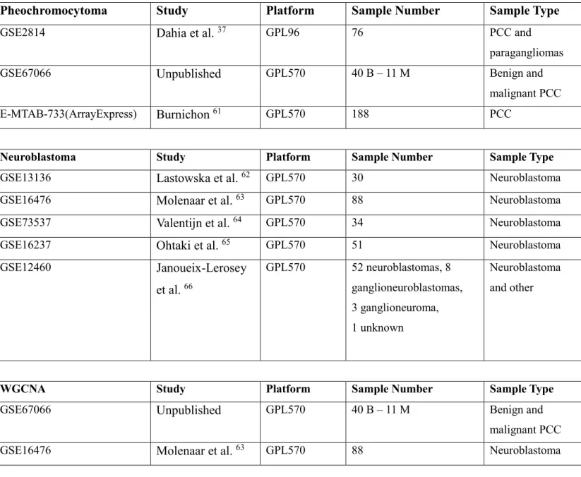
Table 1: The datasets that were acquired from the GEO database and used in further analyses.
3.2. Shiny Application Design
There are multiple ways to define a Shiny application, meaning that it could be formatted in multiple ways. A conventional Shiny application is made up of two parts; a server side and a user interface (UI) side 67. The UI part contains the information to be shown and parts for user
interaction, such as a numeric input box or a boxplot. The server part contains the code that does the computations needed to construct the outputs of the application. Depending on the type of the input/output, varying UI elements are available for use, for instance, using the renderUI()
Pheochromocytoma Study Platform Sample Number Sample Type
GSE2814 Dahia et al. 37 GPL96 76 PCC and
paragangliomas
GSE67066 Unpublished GPL570 40 B – 11 M Benign and
malignant PCC
E-MTAB-733(ArrayExpress) Burnichon 61 GPL570 188 PCC
Neuroblastoma Study Platform Sample Number Sample Type
GSE13136 Lastowska et al. 62 GPL570 30 Neuroblastoma
GSE16476 Molenaar et al. 63 GPL570 88 Neuroblastoma
GSE73537 Valentijn et al. 64 GPL570 34 Neuroblastoma
GSE16237 Ohtaki et al. 65 GPL570 51 Neuroblastoma
GSE12460 Janoueix-Lerosey et al. 66 GPL570 52 neuroblastomas, 8 ganglioneuroblastomas, 3 ganglioneuroma, 1 unknown Neuroblastoma and other
WGCNA Study Platform Sample Number Sample Type
GSE67066 Unpublished GPL570 40 B – 11 M Benign and
malignant PCC
17
command in the server side enables the construction of reactive inputs, according to the previous input given by the user.
There are also numerous ways to structure the layout of a Shiny application. A fairly simple option could be to have a sidebar for inputs and main area for output or a more complex and customizable layout could be accomplished by using the Shiny grid layout system. Another option is to build a segmented structure using the tabsetPanel() and navlistPanel() functions. In addition to the tab-based segmentation method, applications with multiple top-level components can be accomplished with the navbarPage() function. The CoEX-PM application in this thesis uses a hybrid of the aforementioned methods. There are three top-level components that are segmented into multiple tabs individually as described in the following sections.
3.2.1. Tab 1: Pairwise correlation analysis.
Correlation between any two genes can be calculated based on expression of mRNA levels obtained from a high-throughput study. This correlation can be obtained either in the form of parametric or nonparametric formulas, Pearson’s or Spearman’s correlations respectively 68.
The correlation coefficient reflects the degree of similarity in direction and/or relative magnitude of change from point to point (e.g., time to time, tissue to tissue). A positive correlation between a pair of two genes indicates the degree of similarity in co-expression whereas a negative
correlation may indicate opposing actions taking place on the expression of the genes.
In this tab, the aim has been to take as input the names of the genes of interest along with the GEO ID of a dataset before plotting the correlation between expressions of genes using the
cor() and cor.test() functions in tandem in R. The cor() function has been used to calculate the
correlation of a particular probe to all the other probes on the array, whereas the cor.test() function was utilized to establish an association between paired samples of the correlation coefficient vectors of the two genes of interest. The cor() function was the core element of a custom function that takes a gene symbol and a data frame as input returning a two-column data frame with the correlation co-efficient r and p-value as columns, respectively. For plotting purposes, generic plotting functions of R and relevant ggplot2 functions were used 69. In
addition, ggsave() function has been used to save plots in a preferred directory on the local machine.
18
3.2.2. Tab 2: Meta-analysis Tab
In CoEX-PM I have made available meta-analysis of a correlation coefficient between expression of a gene of interest with that of each of the remaining genes in the expression analysis platform from a selected set of GEO datasets. In the previous tabs the required datasets must have been acquired into the Shiny work environment so that the Meta-analysis tab can work.
The main R function used in this module/tab is metacor. This function has been deposited in the CRAN repository 70.
Metacor package
There are two core functions of the metacor package, metacor.DSL() and metacor.OP(). For this study, I have used the metacor.DSL() function which implements the DerSimonian-Laird (DSL) random-effect meta analytical approach where correlation coefficients are treated as effect sizes 71. The parameters of the function have been designed as follows:
metacor.DSL(r, n, labels, alpha = 0.05, plot = TRUE, xlim = c(-1, 1), transform = TRUE)
where r is a vector correlation and n is a vector of sample sizes. The function returns a number of values (mainly the mean effect sizes z.mean/r.mean and their confidence intervals) which are then structured into a data frame object to make it easier to manipulate and visualize the data. The construction of the data frame object as well as some other pre-processing and data acquisition steps have been done by a custom function written by Dr. Huma Shehwana, an alumna of our lab 58.
3.2.3. Tab 3: WGCNA Tab
Weighted gene co-expression network analysis (WGCNA) is a robust method for identifying biologically relevant expression patterns in highly multivariate and complex data, such as microarray datasets 59. Conventionally, network building methods quantify the pairwise
correlations for each gene individually but WGCNA also quantifies the extent to which these pairs of genes share the same neighbors. As a result, a topological overlap matrix is created. The overlap matrix is converted to a dissimilarity matrix which is then subjected to hierarchical clustering 59.
19
This line of computation results in a dendrogram which clusters genes with similar expression patterns into distinct branches and most highly connected nodes or “hubs” are located the branch tips. Furthermore, WGCNA provides ways to cluster these branches into separate “modules” that contain a group of genes with highly covarying expression patterns across the dataset. Each module contains an “eigengene” element corresponding to its expression pattern and genes that are highly correlated with the module eigengene are referred to as “hub” genes. Importantly, by enabling additional genetic, developmental or phenotypic traits to be associated with tens of modules, rather than tens of thousands of variables, WGCNA resolves the multiple testing problem as well as providing a direct way to detect experimental treatment effects in structured networks.
In CoEX-PM I have made available WGCNA analysis to be performed on the selected GEO datasets and identified the modules and found the co-expression clusters associated with the selected genes before performing the relevant plotting. In addition, the main R package to be used is the WGCNA package coupled with the limma package for the pre-processing step of identifying differentially expressed genes 7259.
I have incorporated WGCNA module into the CoEX-PM using a modified version of a conventional WGCNA workflow documented by the authors of the package 59. First of all, to
select the genes to be included in the WGCNA, a differential expression analysis has been conducted. As a result of this analysis, top 10K genes was selected to be included in the WGCNA analysis. This type of gene filtering is required since WGCNA operates optimally working with 10K-20K genes, also any number of genes higher than this band requires a lot of computational power. Therefore, it is not advisable and, in most circumstances, impossible to conduct WGCNA with the whole probe set of a microarray platform.
20
4. Results
4.1. COEX-PM Application
4.1.1 Gene-Correlation Tab
The CoEX-PM application has been uploaded online in the GitHub repository hosting service. It is freely available in GitHub where there are user’s guide documentations as well, explaining the work flow in detail.
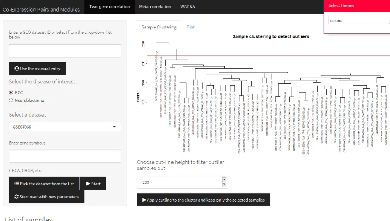
The main screen of the CoEX-PM is provided in Figure 1. The three tabs in this module can be accessed by clicking on the tabs. For exemplary purposes the dataset GSE67066 was selected and uploaded for analyzing one of the NET datasets already have been deposited in the
application. As it is possible to select an existing dataset (PCC or Neuroblastoma options) it is also possible to upload a new dataset to analyze using GSE ID number from GEO 28. Before
analysis of gene pairs this module performs a hierarchical clustering based on hclust function using the sample files starting with GSM allowing the user to select and filter out outliers, if any, from the whole dataset. This can be done by selecting a cut-off point on the branch lengths using
cutreeStatic function in R. In addition, the boxplots of normalized expression values can be
21
22
Once the clustering has been done and samples selected the user can perform the plotting of the genes (Figure 2). This can be done by clicking on the plot tab. On the left panel the gene names to be entered into the plot tab are provided with a ‘-‘ sign in between. As many genes as the user wants can be entered (Figure 2). Once the gene names are uploaded the program allows selection of two of them for doing a scatterplot between the correlation coefficients obtained from the expression values for the selected genes. This page provides relevant information about the procedures, and data used for the plotting, i.e., the probeset IDs, the GSE number, number of samples the dataset contains. In addition, there is an option for coloring using either the p-values or the expression values (mean expression for each probe across all selected samples) based on significance or intensity, respectively. This coloring has been done using the function
scale_colour_gradient2() which creates a diverging color gradient (low-mid-high). When the “Construct the correlation plot” button is pushed a scatter plot is generated by using the ggplot()
function in R. At this point it is important to emphasize that the points on the plot represent the correlation coefficients of selected genes with all the other probes on the array platform, not the signal intensity levels of selected genes. A vector for each inputted gene is created, containing the correlation values with the other genes and these two vectors are visualized on the scatterplot. Overall, the first tab investigates user-inputted gene pairs in terms of how correlated their
correlations with other genes are. A high r value would mean that the genes have a similar correlation pattern in terms of their correlation with other probes and vice versa.
The plot is interactive and this is established by the use of two Shiny functions;
nearPoints() and brushedPoints(). By adding click and brush input objects to a specific plot’s
output command, it is possible to print out the clicked and brushed regions on a plot. When clicked on a point on the plot, nearPoints() function searches the nearby pixels for points on the clicked spot, then returns a list of the relevant points. Similarly, brushedPoints() function searches inside the brushed region for points on plot and prints out the relevant points. For the
CoEX-PM application, r and p values of each clicked-on and/or brushed points are printed out
(Figure 2: Plot part of the Two-Gene Tab). Lastly, “the brushed points table” can be downloaded by pushing the download button at the bottom of the screen.
23
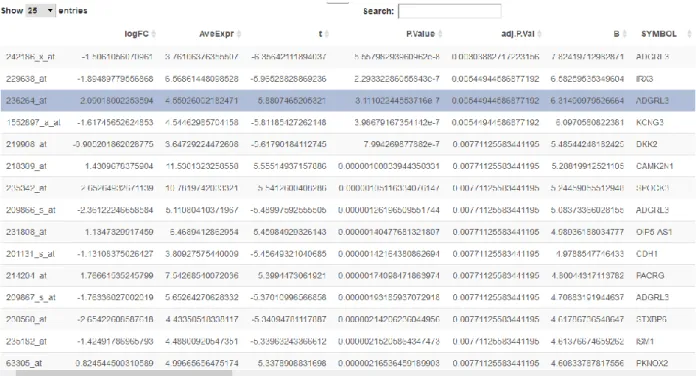
24 4.1.2. Meta-correlation Tab
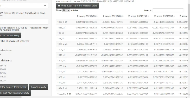
Figure 3: The screenshot of Meta-correlation Tab
The meta-correlation tab does not have sub-tabs unlike the other two main tabs of the application; the two-gene correlation tab and the WGCNA tab. The core output of this tab is the meta-correlation analysis table which is interactable in RStudio or a web browser (Figure 3). The table can be sorted by any selected column by clicking on the column name. In addition, there is a search box that enables quick filtering of the table. Especially for the content of the
“SYMBOL” column, the search box proves useful. The table result can be saved locally by clicking the button on top of table “Write a .csv file of the metacor table”. Consequently, the table is saved in .csv format which is a flexible format to investigate in multiple platforms.
There is a preset list of GEO datasets that the user can choose from or the user could enter a dataset ID manually. The user pushes either the “Use the manual entry” action button to make the manual entry the working dataset list or the “Pick the datasets from the list” action button to designate the preset list of datasets as the working dataset list. Once the gene of interest is also entered, the analysis can be started by clicking on the “Go when ready” button. An initial correlation analysis takes a certain amount of time due to downloading, pre-processing and
meta-25
analysis of fairly large datasets. Once a dataset is used, it is saved locally in a format that makes it faster to use the same dataset in another analysis. Overall, the meta-analysis results are
presented in a tabulated form in which the first column refers to the probeset ID and the metacor program results are provided for each probeset (Figure 3).
4.1.3. WGCNA Tab
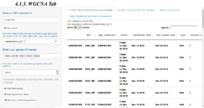
Figure 4: The screenshot of WCGNA Tab: Limma Differential Gene Expression Analysis – Phenodata table.
26
Figure 5: The screenshot of WCGNA Tab: Limma Differential Gene Expression Analysis – limma table.
Array platforms contain tens of thousands of probes and, more often than not, a great number of genes that correspond to these probes might be irrelevant to the researchers. In
addition, WGCNA pipeline computationally struggles when given a number of genes higher than 10-20K. Therefore, I have implemented a proven method of filtering genes by using the limma package. A straight-forward differential gene expression analysis has been conducted prior to WGCNA. Once a dataset ID has been entered, upon the activation the of the “Start pheno” action button, an interactive data table containing phenotypic data elements of the inputted dataset appears on the main panel. This table enables a quick examination of the phenodata to pick a column that is to be used as a grouping factor element for the limma analysis (Figure 4). After selecting a column and clicking on the “Start limma table” button on the side panel, limma analysis results are shown on the main panel (Figure 4). Similar to the phenodata table, the
limma table is also interactable and searchable with a search box (Figure 5). The user is able to
keep the preferred number of top genes (in terms of p-value) for the WGCNA. Lastly, a list of genes of interest are entered which are to be related to the modules in the following analyses. Once the aforementioned processes have been completed, clicking the ‘start expression matrix’
27
action button, the user can move on to the next tab. At this point, the raw data have been normalized, filtered semi-automatically by differential gene expression analysis and user input and a list of genes of interest have been obtained for later steps.
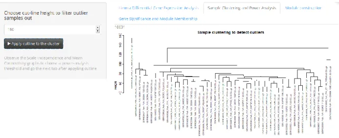
Figure 6: WGCNA Tab: Sample Clustering and Power Analysis – Sample clustering scheme
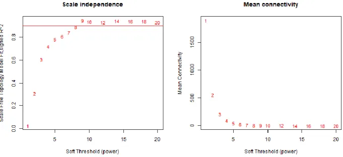
A filtering at the probe level has taken place up to this point but now the samples are clustered to detect any outliers. A cut-off line height can be used to omit the outlier samples (Figure 6). After the numeric input is given and “Apply cutline to the cluster” action button is activated, network topology analysis plots are created. One of the parameters needed to be determined is the soft thresholding power β to which co-expression similarity is raised to calculate adjacency 59. WGCNA package documents suggest that the soft thresholding power
could be selected based on the approximate scale free topology. For this, two plots, scale independence and mean connectivity, can be used to decide on the threshold (Figure 7). This is important since selecting a precise power threshold is required to optimize the sensitivity and specificity of this analysis (Figure 8).
28
Figure 7: Network topology analysis plots for various soft-thresholding powers.
Modules are generated by WGCNA and module colors are shown below the clustergram (Figure 8). The tabs in the WGCNA module also include graphics for gene significance and module membership (Figure 8).
Figure 8: WGCNA Tab: Module Construction – Module dendrogram of genes, each color represents a different module, grey color is reserved for genes that are not a member of any module.
29
4.2. Case-study: Chromogranins in NETs
As explained in detail in the introduction there are up to seven related
chromogranins/secretogranins, i.e., CHGA, CHGB, SCG2, SCG3, and SCG5, in the human genome. These proteins are transcribed from different loci and can form more complex structures post-translationally and take roles in secretion of molecules, including neurotransmitters. One of the primary aims I have focused in this thesis has been to find out whether the chromogranin family members are co-expressed differentially in different cancers in which there are neuroendocrine subtypes.
4.2.1. Pairwise correlations between secretogranin-chromogranin genes
These five secretory components, SCG2, SCG3, SCG5, CHGA and CHGB, have been studied in different GSEs. The expressions of CHGA and CHGB with each other (Figure 9) and with the expression of each of SCG2, SCG3, SCG5 have been identified using CoEX-PM (Figure 10 for GSE67066; Figure 12 for GSE16476; Figure 14 GSE12667; Figure 13 GSE13136; Figure 11 GSE2841).
30
Figure 9: CHGA-CHGB correlation plots for nine distinct datasets. GSE67066, GSE2841 – PCC; GSE13136, GSE16476, GSE16237, GSE12460 – neuroblastoma; GSE39612 – Merkel cell carcinoma; GSE35679 – lung carcinoid, GSE12667 – lung adenocarcinoma.
CHGA and CHGB genes were highly correlated in most of the datasets examined except GSE16476 and GSE16237, two of the neuroblastoma datasets (Figure 9). Interestingly
31
two highly paralogous genes might have diverged in their function based on their co-expression with different sets of genes (Figure 9). In the other datasets in which CHGA and CHGB were expressed the correlation between expression patterns of these genes were sustained.
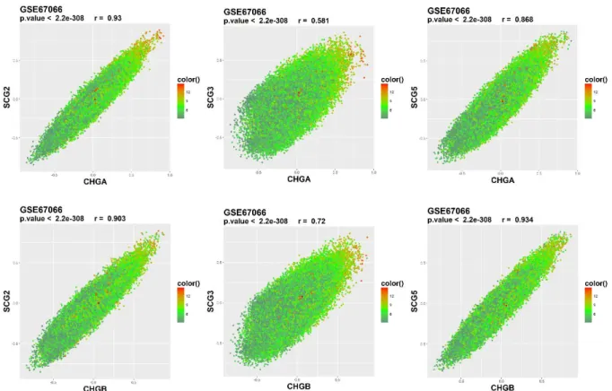
Figure 10: Correlation plots of chromogranins of interest (CHGA-CHGB) with secretogranin genes of interest (SCG2-3-5) for the GSE67066 dataset (PCC, pheochromocytoma). The color gradient implies the expression level.
To examine the correlation between the other three secretogranins in a pairwise fashion, the correlations coefficients of CHGA and CHGB with secretogranins was plotted against those of SCG2, SCG3, and SCG5, respectively. In GSE67066 PCC dataset SCG3 was not as highly correlated with CHGA and CHGB while SCG2 and SCG5 were relatively more correlated with either CHGA or CHGB. Similarly, SCG3 was slightly less correlated to CHGA and CHGB in the GSE2841 PCC dataset (Figure 10). This has suggested that the co-expression network of SCG3
32
could have diverged from the rest of the chromogranin/secretogranin family in PCC.
Figure 11: Correlation plots of chromogranin of interest (CHGA-CHGB) with secretogranin genes of interest (SCG2-3-5) for the GSE2841 dataset. The color gradient implies the expression level. GSE2841 contains 76 pheochromocytoma samples of various genetic origin.
Similarly, as in the other PCC dataset SCG3 behaves relatively less correlated when compared with the other two secretogranins suggesting divergence of expression between secretogranin 3 and the others (Figure 11).
33
Figure 12: Correlation plots of chromogranin of interest (CHGA-CHGB) with secretogranin genes of interest (SCG2-3-5) for the GSE16476 dataset. The color gradient implies the expression level. GSE16476 contains 88 human neuroblastoma samples.
Interestingly, as I have seen the dissociation between CHGA and CHGB co-expression scatterplots SCG2, SCG3, and SCG5 all were negatively correlated with CHGA co-expression values while positively correlated with CHGB co-expression values (Figure 12). This suggests that expression divergence taking place between CHGA and CHGB was mostly driven by the distinctly opposite behavior of CHGA in neuroblastoma while CHGB, SCG2, SCG3, and SCG5 were relatively similar in their co-expression networks.