IS S N 1 3 0 3 –5 9 9 1
SOLUTION OF NONLINEAR SINGULAR BOUNDARY VALUE PROBLEMS USING POLYNOMIAL-SINC APPROXIMATION
MAHA YOUSSEF AND GERD BAUMANN
Abstract. A new highly accurate algorithm for the solution of nonlinear sin-gular boundary value problems for ordinary di¤erential equations is presented. The algorithm uses a collocation technique based on polynomial approxima-tion at Sinc points. The scheme is tested for some nonlinear singular boundary value problems showing an exponential convergence rate. The examples are of second and higher order singular, nonlinear boundary value problems. For each example the error formula of the approximation is discussed and veri…ed in a comparison of the analytic solution.
1. Introduction
The topic of singular boundary value problems has been of rapidly growing in-terest in many applications in science and engineering. A singular problem is found in many important applications, e.g. boundary layer theory, the study of stellar interiors, and control and optimization theory. Some of these problems are linear and others are nonlinear. For the nonlinear singular boundary value problems, many numerical solutions have been discussed in literature [32, 33, 29]. One of the commonly used technique is the series solution [11]. Although this technique is a highly accurate solution it has to be modi…ed and adopted for each single problem according to the type of singularity. On the other hand authors used the shooting method [18] which is based on root …nding methods that need a large number of iterations to get a high accuracy solution. Also, many articles developed Adomian decomposition method [2, 4, 5, 24, 31], and the related modi…cations [21, 32, 33] to investigate various singular nonlinear models. The Adomian decomposition tech-niques have the same disadvantage as polynomial and series solutions that need to be adopted to each di¤erent model. One of the most accurate approximation methods is the use of Sinc approximation [29]. There are two techniques based on
Received by the editors July 21, 2014, Accepted: Sept. 30, 2014. 2010 Mathematics Subject Classi…cation. 34B15; 34B16.
Key words and phrases. Nonlinear singular boundary value problem, polynomial approxima-tion, exponential convergence rate.
c 2 0 1 4 A n ka ra U n ive rsity
Sinc approximation to solve singular boundary value problems, Sinc-Galerkin [29] and Sinc-Collocation methods [9, 29]. Both of these techniques show exponential convergence rate. But, Sinc approximation has a problem in approximating the derivative of the analytic functions on a …nite or semi-in…nite intervals [29]. In this paper, we present a polynomial approximation that overcomes this problem. More over, it keeps the same advantage as Sinc approximation, that it shows an exponential convergence rate.
Now, let us consider the nonlinear di¤erential equations of order m 2: L(u) u(m)+ l1(x; u)u(m 1)+ l2(x; u)u(m 2)+ ::: + (1.1)
lm 1(x; u)u 0
+ lm(x; u) = f (x); a x b
With the boundary conditions:
u(j)(a) = j; u(k)(b) = k; 0 j J; 0 k K and, J + K = m 2 (1.2)
where the functions li(x; u), 1 i m are functions of x and u which are analytic
in [a; b], nonlinear (or linear), and singular (or non-singular). The existence and uniqueness of the solution of (1.1-1.2) is discussed by Agarwal and Akrivis in [6].
2. Collocation of Poly-Sinc Method
In this section we introduce a collocation method based on the polynomial-like approximations at Sinc data. This collocation method reduce the boundary value problems to a system of nonlinear algebraic equations. Without any adaptation of the technique, the collocation method is able to deal with the singularity at the end-points.
It is well known that whitacker’s cardinal function can be used to approximate almost every calculus operation [29]. All of these approximations posses an excep-tionally fast rate of convergence [29]. One of the few shortcomings of Sinc approxi-mation is that it delivers a poor accuracy in the neighborhood of the …nite end-point when di¤erentiating the interpolation Sinc formula on a …nite or semi-in…nite inter-val. This problem has been solved in [27] by introducing polynomial-like methods of approximation. The fortune of this approach is the fact that polynomials as well as their derivatives converge rapidly on a …nite interval for functions that are analytic in a region containing this interval.
2.1. Sinc points and Lagrange polynomial notations. In Lagrange approxi-mation di¤erent sets of points fxk; f (xk)gnk=0are used as interpolation points. The
most famous set of points are the equidistant points but it is well known that these points deliver bad results [30]. To improve the accuracy of Lagrange approximation other sets of points are used, like Chebychev points and modi…ed Chebychev points [26]. Recently it has been shown that it is more e¤ective to use Sinc points as
interpolation points [28]. This sequence of points is created using a conformal map that redistribute the in…nite equidistant points of the real line on a …nite interval locating most of these points near the end-points of the …nite interval. Also, it is proved that using Sinc-points as interpolation points will give a high accurate approximation and allows an accuracy similar to the classical Sinc approximation [27].
To de…ne these interpolation points let Z denote the set of all integers. Let R be the real line, and C denote the complex plane. Let h denote a positive parameter and let k 2 Z, z 2 C.
Let d denote a positive number, and let denote the conformal map of a simply connected region D C onto the strip
Dd= fz 2 C : jIm(z)j < dg:
Let = 1(R) be an arc and let a = 1( 1) and b = 1(1) denote the end points of . Then we de…ne the set of Sinc points by zk = 1(kh), and set
= e (z).
Finally, let 2 (0; 1] and 2(0,1] denote …xed positive numbers, let us restrict d introduced above to the interval (0; ). Let L ; (D) denote the family of all
functions that are analytic in D, such that for all z 2 D, we have ju(z)j c1 j (z)j
[1 + j (z)j] + :
The space of functions M ; (D) denotes the set of all functions g de…ned on D
that have …nite limits g(a) = limz!ag(z) and g(b) = limz!bg(z), where the limits
are taken from within D, and such that u 2 L ; (D), where,
u=g g(a) + g(b)
1 + :;
now we are in position to de…ne a family of polynomial-like approximations that interpolate given Sinc data of the form fxk, u (xk)gNk= M where the xk are Sinc
points. This novel family of Lagrange polynomials was recently derived in [27]. The approximation is accurate, provided that the function u with uk = u (xk) belongs
to a suitable space of analytic functions.
Generally, Lagrange polynomial approximation over the interval [a; b] is de…ned in the following way.
Given a set of n = M + N + 1 distinct points fxkgNk= Mon the interval [a; b] and
function values, fu (xk)gNk= M. Let xk be the Sinc points that are de…ned using
the conformal map (x) = ln((x a)=(b x)) and so the Sinc points can be given by:
xk = 1(kh) =
a + bekh
At these points fxk, u (xk)gNk= M, there exists a unique polynomial p(x) of
degree at most n 1 satisfying,
p (xk) = uk; k = M; ...; N:
In this case p(x) can be expressed as:
p(x) = N X k= M bk(x)uk; (2.2) with, bk(x) = g(x) (x xk) g0(xk) ; (2.3) where, g(x) = N Y j= M (x xj) :
This approximation, like regular Sinc approximation, yields an exceptional ac-curacy in approximating the function that is known at Sinc points. Unlike Sinc approximation, it gives an exponential convergence rate when di¤erentiating the interpolation formula given in (2.2), [27].
For the sake of simplicity of our results, we shall assume here that M = N . Theorem 2.1. Let h = p
N, and let fxkg N
k= Ndenote the Sinc points as de…ned
in (2.1). Let u be in M ; (D), and let p(x) be de…ned as in (2.2). Then there exist
two constants A > 0 and B > 0, independent of N , such that
ju(x) p(x)j A p N B2N exp 2N1 2 2 ! ; (2.4)
Proof. For the proof of (2.4), see [27].
The space M ; (D) is connected with a Hardy space Hp(U), where U is the
unit disk. In Hp(U) the best approximation rate of the form o e cpN has been
obtained [7]. The constant c = 2 in our own estimate is not large as this optimal upper bound of the error discussed in [7] as c = , but it is still an excellent upper bound comparing with the upper bounds in Sinc approximations. The optimal distribution of the sequence of points to be chosen on the interval [a; b] is still an open problem till now [7, 13], but one can see that the approximation we introduced here gives an exceptional upper bound of error. In fact getting an exponential decaying rate of convergence is not only the privilege of this approximation, but dealing e¤ectively without any modi…cation with the singularity at the end points.
2.2. The Poly-Sinc Algorithm. In the next step we set up the collocation method based on the use of Lagrange interpolation at Sinc points. We will replace u(x) in equation (1.1) and (1.2) by the Lagrange polynomial de…ned in (2.2). This will reduce the problem to a system of nonlinear algebraic equations. In the approxi-mation u(x) p(x) = N X k= N bk(x) uk: (2.5)
The 2N + 1, coe¢ cients fukg are determined by substituting u(x) de…ned in
(2.5) into equation (1.1) and (1.2) and evaluating the results at the Sinc points xj= 1(jh); j = N + 1; ...; N 2. This delivers a nonlinear system of 2N 2
equations.
If we use the approximation (2.5) to solve di¤erential equations, not only the unknown function u is needed but also its derivatives. To de…ne an approximation for the …rst and second order derivative, we have to di¤erentiate formula (2.5) with respect to x twice. This results into two n n matrices A = [aj;k] and
C = [cj;k] ; j = N; ...; N and k = N; ...; N , representing the …rst order derivative
and the second order derivative, respectively. For the …rst order derivative, u0(xj) p0(xj) = N X k= N aj;kuk; (2.6) where aj;k= b 0 k(xj) = ( g0(x j) (xj xk)g0(xk) if k 6= j PN l= N;l6=j (xj1xk) if k = j: (2.7)
Theorem 2.2. Let h = =pN , and let fxkgNk= Ndenote the Sinc points as de…ned
in (2.1). Let u be in M ; (D), and let p0(x) be de…ned as in (2.6). Then there exist
two constants C > 0 and D > 0 independent of N , such that
max j= N;:::;Nju 0(x j) p0(xj)j C N D2N exp 2N1 2 2 ! : (2.8)
Proof. For the proof of (2.9), see [27]. For the second order derivative,
u00(xj) p00(xj) = N
X
k= N
cj;kuk: (2.9)
cj;k= b00k(xj) = 8 > > < > > : 2g0(xj) (xj xk)2g0(xk)+ g00(xj) (xj xk)g0(xk) if k 6= j PN n= N PN l= N l;n6=j 1 (xj xl)(xj xn) if k = j: (2.10)
Substituting Equations (2.5), (2.6), (2.8), and (2.10) in (1.1) and (1.2), the problem will be reduced to a nonlinear system of 2N + 1 algebraic equations for 2N + 1 unknowns that can be solved by using Newton’s root …nding method to get the coe¢ cients uk.
The substitution of the expansion coe¢ cients uk into (2.5) delivers the
approxi-mation of the BV problem (1.1) and (1.2).
Beside the given error formulas for the approximation in (6) and (10) we use for practical purposes the error norm relation to compare between two di¤erent solutions. This error formula can be given by:
= ku(x) us(x)k = [ Z b a (u(x) us(x))2dx] 1 2; (2.11)
where u(x) is the analytic solution and us(x) is the approximation obtained from
the Poly-Sinc algorithm.
3. Numerical Results
In this section, we demonstrate the e¤ectiveness of the Poly-Sinc algorithm with several illustrative nonlinear singular examples. For comparison reason, some prob-lems have homogeneous boundary conditions and some other probprob-lems have inho-mogeneous boundary conditions but all of them have a known analytic solutions. For each test example, the absolute error between the exact solution or the analytic approximate solution obtained in one of the references and the results obtained by the Poly-Sinc method.
Example 3.1. Consider the following nonlinear singular boundary value problem, eu(x)u00(x) + 1 x(x 1)u 0(x) + 1 1 xu 2(x) = f (x); 0 x 1; (3.1) u(0) = u(1) = 0; where, f (x) = 1 1 x[ 2x4 4x3+ x2+ 3x 1 x(x2 x + 1) + log 2(x2 x + 1)]:
The di¢ culty of this problem is not only the non linearity but also the existence of the singularity at the end points. This kind of singularity requires a speci…c distribution of interpolation points, to be clustered near the end points. This means
that using Sinc points as interpolation points in the collocation scheme might give a great help to overcome this singularity problem. Equation (3.1) has the exact solution u(x) = log(x2 x + 1).
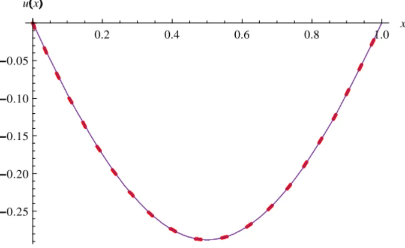
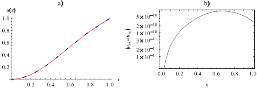
Fig. 1 represents the exact solution, solid line, and the approximate solution, dashed line. For the approximate solution we used n = 2N + 1 = 7 Sinc points.
0.2 0.4 0.6 0.8 1.0 x 0.25 0.20 0.15 0.10 0.05 u x
Figure 1. The exact and approximate solution of Eq. (14) using 7 Sinc points.
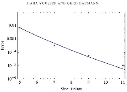
Example 3.2. using the square norm error de…ned in (13), we get an error of 10 4. It is obvious from this result that with a small number of Sinc-points we
get an excellent approximation with a small error. This property is one of the advantages of using Sinc-points as collocation points. To show the property of exponential convergence as regular Sinc method let us present the error function as a function of N only as, CpN E cpN, where C and c are constants. Fig. 2 shows that the norm error based on (13) calculated in this example for di¤erent number of Sinc-points n = 2N + 1 = 5; 7; 9; 11 is satisfying the exponential decaying error function.
If the singularities at the end points exist, it is well known that a large number of collocation points should be used to get an acceptable error. Using the collocation method de…ned in this paper we can see that using a small number of interpolation or collocation points delivers an excellent error. In addition, this error has the property of decaying exponentially as in the classical Sinc approximation.
As in example (3.1), example (3.2) will give another example of nonlinear equa-tions that is de…ned on …nite interval with singularities at the end points.
Figure 2. The error function pN E pN (solid) and the
calcu-lated norm error (dots) for n = 5; 7; 9; 11:
0.2 0.4 0.6 0.8 1.0 x 0.05 0.10 0.15 0.20 0.25 u x a 0.0 0.2 0.4 0.6 0.8 1.0 102 0 101 9 101 8 101 7 101 6 x uex uap b
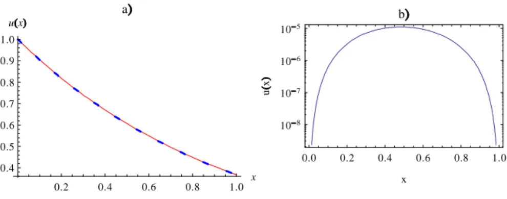
Figure 3. a. The exact and approximate solution of eq. (15) using n = 9, b. The local error juex uapj :
sin(u(x))u00(x) + 1 xp1 xu 0(x) + 1 1 xu 3(x) = f (x); 0 x 1; (3.2) u(0) = u(1) = 0; where, f (x) = 1 2x xp1 x+ r x 1 x 2sin(x x 2):
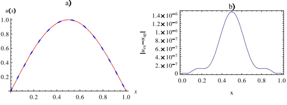
This nonlinear equation (3.2) has singularities at the end points, at x = 0 and x = 1. In addition it has the exact solution u(x) = x x2. As in example
(3.1), we still claiming that using a few number of collocation points will deliver an exponentially small error. To do so, we use n = 2N +1 = 9 Sinc points as collocation points to get, using square norm error (13), an error of 10 16 . In Fig. 3 a., we
represent the exact solution, solid line, and the approximate solution, dashed line. In Fig 3 b. the local error calculated asjuex uapj, where uex represents the exact
solution and uap represents the approximate one at n = 9.
Again in this example we show that using a few number of Sinc points guarantees a very e¢ cient approximate solution, with an error approximately zero.
Next we consider another example of nonlinear boundary value problems over a …nite interval with homogeneous Dirichlet boundary conditions.
0.2 0.4 0.6 0.8 1.0 x 0.2 0.4 0.6 0.8 1.0 u x a 0.0 0.2 0.4 0.6 0.8 1.0 0 2. 107 4. 107 6. 107 8. 107 1. 106 1.2 106 1.4 106 x uex uap b
Figure 4. a. The exact and approximate solution of eq. (16) using n = 9, b. The local error juex uapj :
Example 3.4. Consider the following nonlinear singular boundary value problem [15], p u(x)u00(x) + 30 sin3(x)(1 x2)2(x 0:4)2(x 0:6)u0(x) + (3.3) 1 1 x p
u(x) = f (x); 0 x 1 and u(0) = u(1) = 0;
where f (x) is compatible to the exact solution u(x) = sin( x). This equation contains a singularity at one of the end points, x = 1. To handle such kind of one sided singularity, we need to shift more collocation points near by the end point that includes the singularity. This can be done by using the Sinc points xk = ekh=(ekh+ q) where q = (1 + c)=(1 c) and c is an arbitrary constant in
( 1; 1) [27]. To cluster more Sinc points near by the end point x = 0 we simply choose c 2 (0; 1) and to dense them around x = 1 we choose c 2 ( 1; 0).
Fig. 4 a. represents the exact solution, solid line, and the approximate solution, dashed line. Fig 4 b. the local error calculated asjuex uapj, where uex represents
the exact solution and uap represents the approximate one at n = 9. In [15], Geng
used a reproducing kernel spaces to solve this singular nonlinear boundary value problems. Table 1 gives a comparison between the obtained error in [15] and the recent Poly-Sinc algorithm with the number of used collocation points.
Method Error n
Poly-Sinc (10) 7 9
Reproducing kernel, [15] (10) 5 26 Table 1: Error in example 3.3.
In the last three examples, we were dealing with homogeneous Dirichlet boundary conditions. The next example examines a nonlinear boundary value problems with inhomogeneous boundary conditions.
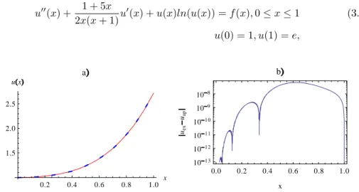
Example 3.5. Consider the following nonlinear singular boundary value problem [23] u00(x) + 1 + 5x 2x(x + 1)u 0(x) + u(x)ln(u(x)) = f (x); 0 x 1 (3.4) u(0) = 1; u(1) = e; 0.2 0.4 0.6 0.8 1.0 x 1.5 2.0 2.5 u x a 0.0 0.2 0.4 0.6 0.8 1.0 101 3 101 2 101 1 101 0 109 108 x uex uap b
Figure 5. a. The exact and approximate solution of eq. (16) using n = 15, b. The local error juex uapj :
Example 3.6. where f (x) is compatible to the exact solution u(x) = (1 x+x2)ex.
For the inhomogeneous boundary conditions, we can collocate the equation (3.4) using xk points where k : N + 1; :::; N + 1. This collocation will deliver 2N + 1
algebraic equations. Then we can add the two boundary equations represented by the polynomial approximation:
p(0) = 1; p(1) = e;
to have a system of 2N + 1 equations in 2N + 1 coe¢ cients.
Fig 5 a. represents the exact solution, solid line, and the approximate solution, dashed line. For the approximate solution we used 15 Sinc points. Fig 5 b. gives the local error calculated at n = 15. For the global error, we use the square norm error de…ned in eq. (13) to get an error of 10 7:
4. Higher Order BVPs
Higher order Boundary Value Problems arise in the mathematical modeling of many physical problems. For example, for a two-dimensional channel with porous walls, viscoelastic and inelastic ‡ows, deformation of beams, plate de‡ection theory, beam element theory and a number of other engineering and applied mathematics applications. Solving such type of boundary value problems analytically is possible only in very rare cases. Many authors worked on the numerical solutions of higher order boundary value problems [11, 15, 25, 16]. Some numerical methods such as …nite di¤erence method, di¤erential transformation method, Adomian’s decom-position method, homotopy perturbation method, variational iteration method, spline methods have been developed for solving such boundary value problems [25, 14, 23, 1]. For Sinc methods, there is not much information available in lit-erature for higher order boundary value problems solved by Sinc methods. For a sixth-order BV problem El-Gamel et al [12] discussed a Sinc-Galerkin method and for fourth-order BV problems Hajii discusses a nonlinear BV problem [19]. Both groups demonstrated the application to a speci…c problem and discuss the convergence properties for this speci…c type of equation. Bialecki in his paper [9] comments on higher order BV problems and states a general formula but does not discuss details of convergence or calculations.
Here we will use the already known algorithm for second order equations and extend this algorithm to an arbitrary higher order algorithm for 1D equations. The theoretical procedure follows the same line as presented for second order equations. However, the method for higher order is di¤erent from the second order method with respect to the incorporation of the boundaries and the discretization of derivatives. Mainly we will discuss four examples. The …rst example is Blasuis equation that is originally introduced in the study of the laminar ‡ow of a ‡uid. The second ex-ample is the fourth order beam equation. The third exex-ample is a nonlinear fourth order boundary value problem. Finally, we discuss the sixth order boundary value problem from [12]. In this example we compare the Poly-Sinc method with the Glarekin Sinc method that is introduced in [12]. This comparison will give an evi-dence that Poly-Sinc is better than some techniques based on Sinc approximations. Example 4.1. Blasius Equation [11]
The Blasius equation is a nonlinear third order di¤erential equation which is given by,
u000(x) + u(x)u00(x) = (u02(x) 1) (4.1) u(0) = u0(0) = 0; u0(x) ! k as x ! 1;
where is an arbitrary constant and k is a constant. When 0, Eq. (4.1) has a unique solution. The original problem with = 0 was solved by H. Blasius [10] who introduced it in the study of the laminar ‡ow of a ‡uid. He found an exact solution of boundary layer equation over a ‡at plate. A more general case 6= 0 has been solved by many authors, for example Howarth [22] solved it by means of numerical methods and many others like Hartree, Falkner, and Skan [11] . Recently, Asaithambi [8] used a …nite di¤erence method to solve Blasius equation. Some other techniques have been adopted to solve the Blasius equation, like Laplace transform and homotopy perturbation method [21] and Adomian decomposition method [1].
Since this equation occupies an important place in the boundary layer problem of hydrodynamics we will give a short background how the original equation of Blasius is constructed.
For a two-dimensional incompressible ‡ow with zero pressure gradient over a ‡at plate the stationary equations for the velocity …elds u and v are giving by:
@u @x+ @v @y = 0 (4.2) u@u @x+ v @v @y = v @2u @y2;
where x is the direction of ‡ow, y the direction of the normal to the plate, u and v the component of the velocity in the directions x and y respectively. The boundary conditions are:
u(x; y = 0) = v(x; y = 0) = 0; u(x; y = 1) = u1
where U is the velocity of the ‡uid. De…ne the following, z = y r U1 v x; = p v x U1f (z);
where f (z) is the dimensionless stream function. Now for the velocity component u, u = @ @y = p v x U1f0(z) r U1 v x = U1f0(z): (4.3)
Also the transverse velocity component can be expressed as, v = @x = 12 r v U1 x (zf 0(z) f (z)): (4.4)
f000(z) + f (z)f00(z) = 0; (4.5) with the boundary conditions:
f (0) = 0; f0(0) = 0; f0(z) ! k as z ! 1: Blasius provided an exact solution in the form,
f (z) = 1 X i=0 ( 1)i i+1 z 3i+2 (3i + 2)!Ai; (4.6)
where Ai is de…ned as:
A0= A1= 1; Ai = i 1 X r=0 3i 1 3r ArAi r 1; i 2;
and = f00(0). For k = 1, Blasius evaluated = 0:332 [10]. Later on Hartree
[20] gained a more accurate value = 0:4696. For k = 2 Howarth [22] computed a …ve decimal value of = 1:32824.
1 2 3 4 5 z 2 4 6 8 10 f z
Figure 6. The approximate(dashed) and analytic solution (solid) of eq. (22) using n = 9.
Example 4.2. Now using Lagrange-Sinc collocation to solve eq. (22) with k = 1. Fig. 6 represents the analytic solution, solid line, in [11] and the approximate solution, dashed line.
Now using equation (13) to calculate the error using the exact solution given in (4.6) as a reference to get an error 10 3 with 9 Sinc points.
Example 4.3. Beam problem
The beam equation which appears in the study of deformation of elastic beams on elastic bearing is a fourth order equations with nonlinear boundary conditions involving third order derivatives. This problem is given by,
u(4)(x) = h(x; u(x)); 0 x 1; (4.7)
u(0) = u0(0) = u00(0) = 0; u000(0) = g(u(1)):
The di¢ culty in this problem is to obtain its numerical solution due to the ap-pearance of third order nonlinear boundary conditions. The existence and unique-ness of the solution for eq. (4.7) has been discussed by Gupta in [17]. Recently, Geng [14] and Silva [25] introduced two di¤erent iterative methods for solving eq (4.7). We will solve this problem using the algorithm proposed in section 2 and showing, numerically, that using Poly-Sinc collocation method will produce much better approximation than these methods exist in [14] and [25]. To solve eq. (4.7) consider h(x; u) and g(u) as [14]:
h(x; u) = u2 x10+ 4x9 4x8 4x7+ 8x6 4x4+ 120x 48; g(u) = 12u: (4.8) Eq. (4.7) together with eq. (4.8) has the exact solution u(x) = x5 2x4+ 2x2 [14]. In Fig 7, we represent the exact solution, solid line, and the approximate solution, dashed. For the approximate solution we used 11 Sinc points.
0.2 0.4 0.6 0.8 1.0 x 0.2 0.4 0.6 0.8 1.0 u x a 0.0 0.2 0.4 0.6 0.8 1.0 1 101 1 2 101 1 5 101 1 1 101 0 2 101 0 5 101 0 x uex uap b
Figure 7. a. The exact and approximate solution of eq. (24) using n = 11, b. The local error juex uapj :
Example 4.4. Using the square norm error de…ned in eq (13), we get error of 10 10. Table 2 includes the errors obtained using Poly-Sinc and other techniques
Method Error
Poly-Sinc (10) 10
Contraction principle, [25] (10) 2 Reproducing kernel, [14] (10) 3
Table 2: Error in example 4.2.
Example 4.5. Consider the following fourth order boundary value problems [16]
u4(x) + 4u(x) = 1; 1 x 1; (4.9)
with the boundary conditions,
u( 1) = u(1) = 0;
u0( 1) = u0(1) = sinh 2 sin 2 4(cosh 2 + cos 2)
Gupta used cubic B-spline to solve this fourth order boundary value problems [16]. Here we will use the Poly-Sinc algorithm to solve (25).
0.2 0.4 0.6 0.8 1.0 x 0.4 0.5 0.6 0.7 0.8 0.9 1.0 u x a 0.0 0.2 0.4 0.6 0.8 1.0 108 107 106 105 x u x b
Figure 8. a. The exact and approximate solution of eq. (27) using n = 13, b. The local error juex uapj :
Example 4.6. Table 3 includes the obtained error using Poly-Sinc and the error obtained in [16].
Method Error
Poly-Sinc (10) 10
Cubic B-spline, [16] (10) 6
Table 3: Error in example 4.3.
u(6)(x) + e xu2(x) = e x+ ex; 0 x 1; (4.10) u(0) = 1; u0(0) = 1; u00(0) = 1; u(1) = 1 e; u 0(1) = 1 e; u 00(1) = 1 e:
this equation has the exact solution u(x) = e x. This Problem was discussed by
Zayed and Gamel [12]. They presented a Sinc-Glarekin method to solve nonlinear boundary value problems with di¤erent types of boundary conditions. For this example Zayed and Gamel used 33 Sinc-points to achieve an error 10 3. Here
we will use the Poly-Sinc technique to show that with much smaller number of Sinc-points we can achieve a better approximation.
Fig 9 represents the exact solution, solid line, and the approximate solution, dashed. For the approximate solution we used 13 Sinc points. Using the square norm error de…ned in eq (13), we get an error of 10 6. This means that we used less
than half of the points that Zayed used to double the accuracy of the approximate solution.
5. Conclusion
The Poly-Sinc collocation technique is used to obtain accurate numerical solu-tions of nonlinear boundary value problems with homogeneous and inhomogeneous boundary conditions. This technique needs very little computational e¤ort concern-ing only the solution of an algebraic nonlinear system of equations. Two advantages of this technique have been introduced here. The …rst advantage is that the tech-nique can deal easily with di¤erent types of singularity at the boundaries without any modi…cation of the technique. The second advantage is the exponential conver-gence of this solution that is reaching the optimal upper bound of that are discussed in all Sinc approximations. Finally, we demonstrated that this technique is much more e¤ective than the other techniques that are used to solve the equations dis-cussed in the examples.
References
[1] S. Abbasbandy, Numerical solutions of the integral equations: Homotopy perturbation method and Adomian’s decomposition method, Appl. Math. Comput., Vol. 173, pp. 493–500, (2006). [2] G. Adomian, A review of the decomposition method and some recent results for nonlinear
equation, Math. Comput. Modelling Vol. 13(7), 17-43, (1990).
[3] G. Adomian, Solving frontier problems of physics: The Decomposition Method, Kluwer, Boston, MA, (1994).
[4] G. Adomian and R. Rach, Noise terms in decomposition series solution, Com- put. Math. Appl., Vol. 24(11) (1992).
[5] G. Adomian, R. Rach and N.T. Shawagfeh, On the analytic solution of the Lane-Emden equation, Found. Phys. Lett., Vol. 8(2), 161-181, (1995).
[6] R.P. Agarwal, G. Akrivis, Boundary value problems occuring in plate de‡ection theory, Jour-nal of ComputatioJour-nal and Applied Mathematics, Vol. 8, pp. 145–154, (1982).
[7] J. E. Anderson, B.D. Bojanov, A Note on The Optimal Quadrature in Hp, Numer. Math., Vol. 44, 301-308, (1984).
[8] A. Asaithambi, A Finite-di¤ erence Method for the Falkner-Skan Equation, Appl. Math. Comp., Vol. 92, pp. 135–141, (1998).
[9] B. Bialecki, Sinc-Collocation Methods for Two-Point Boundary Value Problems, IMA J. Num. Anal., Vol. 11, 357-375, (1991).
[10] H. Balsius The boundary layers in ‡uid with little friction, Zeitschrift f•ur Mathematik und Physik, Vol. 56, no. 1,908, pp. 1-37 (1908).
[11] H.T. Davis, Introduction to Nonlinear Di¤ erential and Integral Equations, Dover, New York, (1962).
[12] M. El-Gamel, J. R. Cannon, A. I. Zayed, Sinc-Galerkin Method for Solving Linear Sixth-Order Boundary-Value Problems, Math. Comp., Vol. 73, 1325-1343, (2003).
[13] P. Erdös, Problems and results on the theory of interpolation. II, Acta Math. Hungar., Vol. 12, pp. 235-244, (1961).
[14] F. Geng Iterative reproducing kernel method for a beam equation with third-order nonlinear boundary conditions, Mathematical sciences, a springer open journal (2012)
[15] F. Geng and M. Cui, Solving Singular Nonlinear Two-Point Boundary Value Problems In The Reproducing Kernel Space, J. Korean Math. Soc., Vol. 45 , No. 3, pp. 631-644 (2008). [16] Y. Gupta and P. K. Srivastava, A Computational Method for Solving Two Point Boundary
Value Problems of Order Four, J. Comp. Tech. Appl., Vol 2(5), pp. 1426-1431, (2011). [17] C.P. Gupta, Existence and Uniqueness Theorems for the Bending of an Elastic Beam
Equa-tion, Applicable Anulvis., Vol. 26, pp. 289-304, (1988).
[18] S. N. Ha, A Nonlinear Shooting Method for Two-Point Boundary Value Problems, Int. J. Computers and Mathematics with Applications, Vol. 42, pp. 1411-1420, (2000).
[19] M. Hajji, K. El-Khaled, Numerical methods for non-linear fourth-order boundary value problems with applications, International Journal of Computer Mathematics, vol. 85, No.1, Jan.2008, 83-104.
[20] D. R. Hartree, On an Equation Occurring in Falkner and Skan’s Approximate Treatment of the Equations of the Boundary Layer, Proc. Cambridge Phil. Soc., Vol. 33, pp. 223-239, (1937).
[21] M. M. Hosseini, Adomian decomposition method with Chebyshev polynomials, Appl. Math. Comput., Vol. 175 , 1685-1693, (2006).
[22] L. Howarth, On the Solution of the Laminar Boundary Layer equation, Proc. Royal Soc. of London, Vol. 164 (A), pp. 547-579, (1937).
[23] M. Jafari, M. Hosseini and S. Mohyud-Din Solutions of nonlinear singular initial value prob-lems by modi…ed homotopy perturbation method, International Journal of the Physical Sci-ences, Vol. 6(6), pp. 1528-1534, 18 March, (2011).
[24] R. Rach, A. Baghdasarian and G. Adomian, Di¤ erential equations with singular coe¢ cients, Appl. Math. Comput., Vol. 47, 179-184, (1992).
[25] Ma, TF, Silva, JD: Iterative solutions for a beam equation with nonlinear boundary conditions of third order. Applied Mathematics and Computation., Vol. 159, 11–18 (2004).
[26] S.J. Smith, Lebesgue constants in polynomial interpolation, Ann. Math. Inform., Vol. 33, pp. 109-123, (2006).
[27] F. Stenger, M. Youssef, and J. Niebsch, Improved Approximation via Use of Transforma-tions : In: Multiscale Signal Analysis and Modeling, Eds. X. Shen and A.I. Zayed, NewYork: Springer, pp. 25-49, (2013).
[28] F. Stenger, H. A. El-Sharkawy and, G. Bauamnn, The Lebesgue Constant for Sinc Approxi-mations, New Perspectives on Approximation and Sampling Theory - Festschrift in the honor of Paul Butzer’s 85th birthday. Eds. A. Zayed and G. Schmeisser, Birkhaeuser, Busel, (2014). [29] F. Stenger, Handbook of Sinc Methods, CRC Press , (2010).
[30] P. V´ ertesi, On a problem of J. Szabados, Acta Mathematica Hungarica, Vol. 28(1), pp. 139-143, (1976).
[31] A. M. Wazwaz, A First Course in Integral Equation, World Scienti…c, Singapore, (1997). [32] A. M. Wazwaz, Analytical approximations and Pade approximations for Volterra’s population
model, Appl. Math. Comput., Vol. 100, 13-25, (1999)
[33] A. M. Wazwaz, A new method for solving singular initial value problems in the second-order ordinary di¤ erential equations , Appl. Math. Comput., Vol. 128, 45-57, (2002).
Current address : Maha Youssef :Mathematics Department, Faculty of Basic Science, German University in Cairo, New Cairo City 11835, Egypt
E-mail address : [email protected]