Image segmentation algorithms for land categorization

16. Image Segmentation Algorithms for Land Categorization

CONTENTS

16.1. Introduction

16.2. Spectrally-based Segmentation Approaches 16.2.1. Thresholding-based Algorithms 16.2.2. Clustering-based Algorithms 16.2.3. Support Vector Machines

16.3. Spatially-based Segmentation Approaches 16.3.1. Region Growing Algorithms

16.3.1.1. Seeded Region Growing

16.3.1.2. Split and Merge Region Growing

16.3.1.3. Hybrid of Spectral Clustering and Region Growing 16.3.1.4 Dissimilarity Criterion and Specialized Control Logic

16.3.1.5. Selection of a Single Segmentation from a Segmentation Hierarchy 16.3.2. Texture-based Algorithms

16.3.3. Morphological Algorithms 16.3.3.1. Watershed Algorithms 16.3.3.2. Morphological Profiles 16.3.4. Graph-based Algorithms

16.3.4.1. Optimal Spanning Forests 16.3.4.2. Normalized Cuts

16.3.5. MRF-based Algorithms

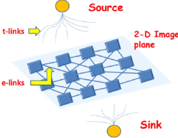
16.3.5.1. Simulated Annealing and Iterated Conditional Modes 16.3.5.2. Graph-cuts

16.4. Image Segmentation Quality Evaluation 16.5. Concluding Remarks

References

16.1. Introduction

Image segmentation is the partitioning of an image into related meaningful sections or regions. Segmentation is a key first step for a number of image analysis approaches. The nature and quality of the image segmentation result is a critical factor in determining the level of performance of these image analysis approaches. It is expected that an appropriately designed image segmentation approach will provide a better understanding of a landscape, and/or

significantly increase the accuracies of a landscape classification. An image can be partitioned in several ways, based on numerous criteria. Whether or not a particular image partitioning is useful depends on the goal of the image analysis application that is fed by the image segmentation result.

The focus of this chapter is on image segmentation algorithms for land categorization. Our image analysis goal will generally be to appropriately partition an image obtained from a remote sensing instrument on-board a high flying aircraft or a satellite circling the earth or other planet. An example of an earth remote sensing application might be to produce a labeled map that divides the image into areas covered by distinct earth surface covers such as water, snow, types of natural vegetation, types of rock formations, types of agricultural crops and types of other man created development. Alternatively, one can segment the land based on climate (e.g.,

temperature, precipitation) and elevation zones. However, most image segmentation approaches do not directly provide such meaningful labels to image partitions. Instead, most approaches produce image partitions with generic labels such as region 1, region 2, and so on, which need to be converted into meaningful labels by a post-segmentation analysis.

An early survey on image segmentation grouped image segmentation approaches into three categories (Fu and Mui, 1981): (i) characteristic feature thresholding or clustering, (ii) boundary detection, and (iii) region extraction. Another early survey (Haralick and Shapiro, 1985) divides region extraction into several region growing and region split and merge schemes. Both of these surveys note that there is no general theory of image segmentation, most image segmentation approaches are ad hoc in nature, and there is no general algorithm that will work well for all images. This is still the case even today.

We start our image segmentation discussion with spectrally-based approaches,

corresponding to Fu and Mui’s characteristic feature thresholding or clustering category. We include here a description of support vector machines, as a supervised spectral classification approach that has been a popular choice for analyzing multispectral and hyperspectral images (images with several tens or even hundreds of spectral bands). We then go on to describe a number of spatially-based image segmentation approaches that could be appropriate for land categorization applications, generally going from the simpler approaches to the more

complicated and more recently developed approaches. Here our emphasis is guided by the prevalence of reported use in land categorization studies. We then take a brief look at various approaches to image segmentation quality evaluation, and include a closer look at a particular empirical discrepancy approach with example quality evaluations for a particular remotely sensed hyperspectral data set and selected image segmentation approaches. We wrap up with some concluding comments and discussion.

16.2. Spectrally-based Segmentation Approaches

The focus of this section is on approaches that are mainly based on analyses of individual pixels. These approaches use an initial labeling of pixels using unsupervised or supervised classification methods, and then try to group neighboring pixels with similar labels using some form of post-processing to produce segmentation results.

16.2.1. Thresholding-based Algorithms

Thresholding has been one of the oldest and most widely used techniques for image

segmentation. Thresholding algorithms used for segmentation assume that the pixels that belong to the objects of interest have a property whose values are substantially different from those of

the background, and aim to find a good set of thresholds that partition the histogram of this property into two or more non-overlapping regions (Sezgin and Sankur, 2004). While the spectral channels can be directly used for thresholding, other derived properties of the pixels are also commonly used in the literature. For example, Akcay and Aksoy (2011) used thresholding of the red band to identify buildings with red roofs, Bruzzone and Prieto (2005) performed change detection by thresholding the difference image, Rosin and Hervas (2005) used thresholding of the difference image for determining landslide activity, Aksoy, et al. (2010) applied thresholding to the normalized difference vegetation index (NDVI) for segmenting vegetation areas, and Unsalan and Boyer (2005) combined thresholding of NDVI and a shadow-water index to identify potential building and street pixels in residential regions.

Selection of the threshold values is often done in an ad hoc manner usually when a single property is involved, but optimal values can also be found by employing exhaustive or stochastic search procedures that look for the values that optimize some criteria on the shape or the

statistics of the histogram such as minimization of the within-class variance and maximization of the between-class variance (Otsu, 1979). A stochastic search procedure is particularly needed for finding multiple thresholds where an exhaustive search is not computationally feasible due to the combinatorial increase in the number of candidate values. For example, a recent use of multilevel thresholding for the segmentation of Earth observation data is described in (Ghamisi, et al., 2014) where a particle swarm optimization based stochastic search algorithm was used to obtain a multilevel thresholding of each spectral channel independently by maximizing the

corresponding between-class variance.

Even when the selected thresholds are obtained by optimizing some well-defined criteria on the distributions of the properties of the pixels, they do not necessarily produce operational

image segmentation results because they suffer from the lack of the use of spatial information as the decisions are independently made on individual pixels. Thus, thresholding is usually applied as a pre-processing algorithm, and various post-processing methods such as morphological operations are often applied to the results of pixel-based thresholding algorithms as discussed in the following section.

16.2.2. Clustering-based Algorithms

The clustering-based approaches to image segmentation aim to make use of the rich

literature on data grouping and/or partitioning techniques for pattern recognition (Duda, Hart and Stork, 2001). It is intuitive to pose the image segmentation problem as the clustering of pixels, and thus, pixel-based image analysis techniques in the remote sensing literature have found natural extensions to image segmentation. In the most widely used methodology, first, the spectral feature space is partitioned and the individual pixels are grouped into clusters without regard to their neighbors, and then, a post-processing step is applied to form regions by merging neighboring pixels having the same cluster label by using a connected components labeling algorithm.

The initial clustering stage commonly employs well-known techniques such as k-means (Aksoy and Akcay, 2005), fuzzy c-means (Shankar, 2007), and their probabilistic extension using the Gaussian mixture model estimated via expectation-maximization (Fauvel, et al., 2013). Since no spatial information is used during the clustering procedure, pixels with the same cluster label can either form a single connected spatial region, or can belong to multiple disjoint regions that are assigned different labels by the connected components labeling algorithm. This reduces the significance of the difficulty of the user's a priori selection of the number of clusters in many popular clustering algorithms as there is no strict correspondence between the initial number of

clusters and the final number of image regions. However, it still has a high potential of producing an oversegmentation consisting of noisy results with isolated pixels having labels different from those of their neighbors due to the lack of the use of spatial data.

Therefore, a following post-processing step aims to produce a smoother and spatially

consistent segmentation by converting the pixel-based clustering results into contiguous regions. A popular approach is to use an additional segmentation result (often also an oversegmentation), and to use a majority voting procedure for spatial regularization by assigning each region in the oversegmentation a single label that is determined according to the most frequent cluster label among the pixels in that region (Fauvel, et al., 2013). An alternative approach is to use an iterative split-and-merge procedure as follows (Aksoy, et al., 2005), (Aksoy, 2006):

1) Merge pixels with identical labels to find the initial set of regions and mark these regions as foreground,

2) Mark regions with areas smaller than a threshold as background using connected components analysis,

3) Use region growing to iteratively assign background pixels to the foreground regions by placing a window at each background pixel and assigning it to the class that occurs the most in its neighborhood.

This procedure corresponds to a spatial smoothing of the clustering results. The resulting regions can be further processed using mathematical morphology operators to automatically divide large regions into more compact sub-regions as follows:

1) Find individual regions using connected components analysis for each cluster, 2) For all regions, compute the erosion transform and repeat:

b) Find connected components of the thresholded image, c) Select sub-regions that have an area smaller than a threshold, d) Dilate these sub-regions to restore the effects of erosion,

e) Mark these sub-regions in the output image by masking the dilation using the original image,

until no more sub-regions are found,

3) Merge the residues of previous iterations to their smallest neighbors.

Even though we focused on producing segmentations using clustering algorithms in this section, similar post-processing techniques for converting the pixel-based decisions into

contiguous regions can also be used with the outputs of pixel-based thresholding (Section 16.2.1) and classification (Section 16.2.3) procedures (Aksoy, et al., 2005).

It is also possible to pose clustering, and the corresponding segmentation, as a density estimation problem. A commonly used algorithm that combines clustering with density estimation and segmentation is the mean shift algorithm (Comaniciu and Meer, 2002). Mean shift is based on nonparametric density estimation where the local maxima (i.e., modes) of the density can be assumed to correspond to clusters. The algorithm does not require a priori knowledge of the number of clusters in the data, and can identify the locations of the local maxima by a set of iterations. These iterations can be interpreted as the shifting of points toward the modes where convergence is achieved when a point reaches a particular mode. The shifting procedure uses a kernel with a scale parameter that determines the amount of local smoothing performed during density estimation. The application of the mean shift procedure to image segmentation uses a separate kernel for the feature (i.e., spectral) domain and another kernel for the spatial (i.e., pixel) domain. The scale parameter for the spectral domain can be estimated by

maximizing the average likelihood of held-out data. The scale parameter for the spatial domain can be selected according to the amount of compactness or oversegmentation desired in the image, or can be determined by using geospatial statistics (e.g., by using semivariogram-based estimates) (Dongping, et al., 2012). Furthermore, agglomerative clustering of the mode estimates can be used to obtain a multi-scale segmentation.

16.2.3. Support Vector Machines

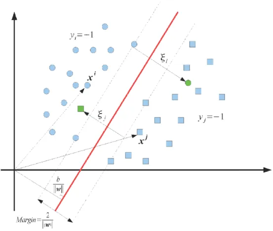
Output of supervised classification of pixels can also be used as input for segmentation techniques. In recent years, support vector machines (SVM) and the use of kernels to transform data into a new feature space where linear separability can be exploited have been proposed. The SVM method attempts to separate training samples belonging to different classes by tracing maximum margin hyperplanes in the space where the samples are mapped. SVM have shown to be particularly well suited to classify high-dimensional data (e.g. hyperspectral images) when a limited number of training samples is available (Camps-Valls, 2005), (Vapnik, 1998). The success of SVM for pixel-based classification has led to its subsequent use as part of image segmentation methods. Thus we discuss the SVM approach in detail below.

SVM are primarily designed to solve binary tasks, where the class labels take only two values: 1 or -1. Let us consider a binary classification problem in a B-dimensional space ℝ , with N training samples, ∈ ℝ , and their corresponding class labels = ±1 available. The SVM technique consists in finding the hyperplane that maximizes the margin, i.e., the distance to the closest training data points in both classes (see Figure 16-1). Noting ∈ ℝ as the vector normal to the hyperplane and ∈ ℝ as the bias, the hyperplane H is defined as

Figure 16-1. Schematic illustration of the SVM binary classification method. There is one non-linearly separable sample in each class.

If ∉ then

( ) = | ∙ + |

∥ ∥

defines the distance of the sample x to H. In the linearly separable case, such a hyperplane must satisfy:

The optimal hyperplane is the one that maximizes the margin 2/∥ ∥. This is equivalent to minimizing ∥ ∥/2 and leads to the quadratic optimization problem:

min ∥ ∥ , subject to (16-1). (16-2)

To take into account non-linearly separable data, slack variables are introduced to deal with misclassified samples (see Figure 16-1). Equation (16-1) becomes

( ∙ + ) > 1 − , ≥ 0, ∀ ∈ [1, ]. (16-3) The final optimization problem is formulated as

min ∥ ∥ + ∑ , subject to (16-3). (16-4)

where the constant C is a regularization parameter that controls the amount of penalty. This optimization problem is typically solved by quadratic programming (Vapnik, 1998). The classification is further performed by computing = ( ∙ + ), where ( , b) are the hyperplane parameters found during the training process and is an unseen sample.

One can notice that the pixel vectors in the optimization and decision rule equations always appear in pairs related through a scalar product. These products can be replaced by nonlinear functions of the pairs of vectors, essentially projecting the pixel vectors in a higher dimensional space ℍ and thus improving linear separability of data:

ℝ ⟶ ℍ ,

⟶ Φ( ) , (16-5) ∙ ⟶ Φ( ) ∙ Φ( ) = ( , ).

Here, Φ(∙) is a nonlinear function to project feature vectors into a new space, (∙) is a kernel function, which allows one to avoid the computation of scalar products in the transformed space [Φ( ) ∙ Φ( )] and thus reduces the computational complexity of the algorithm. The

kernel K must satisfy Mercer's condition (Burges, 1998). The Gaussian Radial Basis Function (RBF) kernel is the most widely used for remote sensing image classification:

( , ) = exp[− ∥ − ∥ ], (16-6) where is the spread of the RBF kernel.

To solve the K-class problem, various approaches have been proposed. Two main approaches combining a set of binary classifiers are defined as (Smola, 2002):

 One versus all: K binary classifiers are applied on each class against the others. Each pixel is assigned to the class with the maximum output ( ).

 One versus one: ( − 1)/2 binary classifiers are applied on each pair of classes. Each pixel is assigned to the class winning the maximum number of binary

classification procedures.

As a conclusion, SVM directly exploit the geometrical properties of data, without involving a density estimation procedure. This method has proven to be more effective than other

nonparametric classifiers (such as neural networks or the k-Nearest Neighbor classifier (Duda, Hart, & Stork, 2001)) in terms of classification accuracies, computational complexity and robustness to parameter setting. SVM can efficiently handle high-dimensional data, exhibiting low sensitivity to the Hughes phenomenon (Hughes, 1968). Finally, it exhibits good

generalization capability, fully exploiting the discrimination capability of available training samples.

Pixel-based supervised classification results, such as those obtained using an SVM classifier, are often given as input to segmentation procedures that aim to group the pixels to form

16.3. Spatially-based Segmentation Approaches

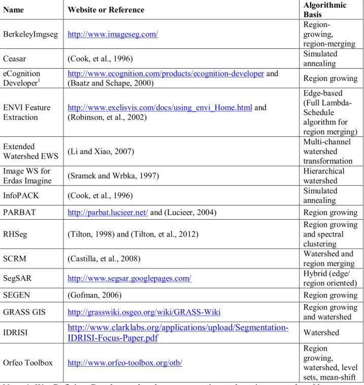
We cannot possibly discuss myriad of spatially-based image segmentation approaches that have been proposed and developed over the years. Instead we will focus on approaches that have achieved demonstrated success in remote sensing land categorization applications. A compilation of such approaches can be found in a series of papers published by a research group based at the Leibniz Institute for Ecological and Regional Development (IOER) that present comparative evaluations of image segmentation approaches implemented in various image analysis packages (Meinel and Neubert, 2004), (Neubert, et al., 2006), (Neubert, et al., 2008), (Marpu, et al., 2010). Table 16.1 provides a summary listing of most of the remote sensing oriented image analysis packages whose image segmentation approach was evaluated in these papers, plus image segmentation approaches from three additional notable remote sensing oriented image analysis packages (GRASS GIS, IDRISI and the Orfeo toolbox).

We note from Table 16.1 that region growing is the most frequent image segmentation approach utilized by these remote sensing oriented image analysis software packages. Further, several packages combine region growing with other techniques (RHSeg with spectral clustering, SCRM and GRASS GIS with watershed, SegSAR with edge detection). Watershed segmentation (an approach based on region boundary detection) is the next most popular approach. Simulated annealing is often utilized in analysis packages oriented towards analyzing Synthetic Aperture Radar (SAR) imagery data (Ceasar and InfoPACK).

The next several sections describe various spatially-based image segmentation approaches, starting with region growing algorithms, and continuing with texture-based algorithms,

Table 16.1. The algorithmic basis of image segmentation approaches in remote sensing oriented image analysis packages. Most of these image segmentation approaches were evaluated in a series of papers by the Leibnitz IOER group.

Name Website or Reference Algorithmic

Basis

BerkeleyImgseg http://www.imageseg.com/

Region-growing, region-merging

Ceasar (Cook, et al., 1996) Simulated

annealing eCognition

Developer1

http://www.ecognition.com/products/ecognition-developer and

(Baatz and Schape, 2000) Region growing

ENVI Feature Extraction http://www.exelisvis.com/docs/using_envi_Home.html and (Robinson, et al., 2002) Edge-based (Full Lambda-Schedule algorithm for region merging) Extended

Watershed EWS (Li and Xiao, 2007)

Multi-channel watershed transformation Image WS for

Erdas Imagine (Sramek and Wrbka, 1997)

Hierarchical watershed

InfoPACK (Cook, et al., 1996) Simulated

annealing

PARBAT http://parbat.lucieer.net/ and (Lucieer, 2004) Region growing

RHSeg (Tilton, 1998) and (Tilton, et al., 2012)

Region growing and spectral clustering

SCRM (Castilla, et al., 2008) Watershed and

region merging

SegSAR http://www.segsar.googlepages.com/ Hybrid (edge/

region oriented)

SEGEN (Gofman, 2006) Region growing

GRASS GIS http://grasswiki.osgeo.org/wiki/GRASS-Wiki Region growing

and watershed

IDRISI

http://www.clarklabs.org/applications/upload/Segmentation-IDRISI-Focus-Paper.pdf Watershed

Orfeo Toolbox http://www.orfeo-toolbox.org/otb/

Region growing, watershed, level sets, mean-shift

Note: 1. Was Definiens Developer – but the remote sensing package is now marketed by Trimble, and the Definiens product is now oriented to biomedical image analysis.

16.3.1. Region Growing Algorithms

In the region growing approach to image segmentation an image is initially partitioned into small region objects. These initial small region objects are often single image pixels, but can also be nn blocks of pixels or another partitioning of the image into small spatially connected region objects. Then pairs of spatially adjacent region objects are compared and merged together if they are found to be similar enough according to some comparison criterion. The underlying

assumption is that region objects of interest are several image pixels in size and relatively homogeneous in value. Most region growing approaches can operate on either grey scale, multispectral or hyperspectral image data, depending on the criterion used to determine the similarity between neighboring region objects.

A very early example of region growing was described in (Muerle and Allen, 1968). Muerle and Allen experimented with initializing their region growing process with region objects consisting of 22 up to 88 blocks of pixels. After initialization, they started with the region object at the upper left corner of the image and compared this region object with the neighboring region objects. If a neighboring region object was found to be similar enough, the region objects were merged together. This process was continued until no neighboring region objects could be found that were similar enough to be merged into the region object that was being grown. Then the image was scanned (left-to-right, top-to-bottom) to find an unprocessed region object, i.e., a region object that not yet been considered as an initial object for region growing or merged into a neighboring region. If an unprocessed region object was found, they conducted their region growing process from that region object. This continued until no further unprocessed region objects could be found, upon which point the region growing segmentation process was considered completed.

Many early schemes for region growing, such as Muerle and Allen’s, can be formulated as logical predicate segmentation, defined in (Zucker, 1976) as:

A segmentation of an image X can be defined as a partition of X into R disjoint subsets X1, X2, …, XR, such that the following conditions hold:

1) ⋃ = ,

2) Xi, i = 1, 2, …, R are connected,

3) P(Xi) = TRUE for i = 1, 2, …, R, and

4) P( ⋃ ) = FALSE for i ≠ j, where Xi and Xj are adjacent.

P(Xi) is a logical predicate that assigns the value TRUE or FALSE to Xi, depending

on the image data values in Xi.

These conditions are summarized in (Zucker, 1976) as follows: The first condition requires that every picture element (pixel) must be in a region (subset). The second condition requires that each region must be connected, i.e. composed of contiguous image pixels. The third condition determines what kind of properties each region must satisfy, i.e. what properties the image pixels must satisfy to be considered similar enough to be in the same region. Finally, the fourth

condition specifies that any merging of adjacent regions would violate the third condition in the final segmentation result.

Several researchers in this early era of image segmentation research, including Muerle and Allen, noted some problems with logical predicate segmentation. For one, the results were very dependent on the order in which the image data was scanned. Also, the statistics of a region object can change quite dramatically as the region is grown, making it possible that many adjacent cells that were rejected for merging early in the region growing process would have been accepted in later stages based on the changed statistics of the region object. The reverse was

also possible, where adjacent cells that were accepted for merging early in the region growing process would have been rejected in later stages.

Subsequently, an alternate approach to region growing was developed that avoids the above mentioned problems, and approach that eventually became to be referred to as best merge region growing. An early version of best merge region growing, hierarchical step-wise optimization (HSWO), is an iterative form of region growing, in which the iterations consist of finding the most optimal or best segmentation with one region less than the current segmentation (Beaulieu and Goldberg, 1989). The HSWO approach can be summarized as follows:

i. Initialize the segmentation by assigning each image pixel a region label. If a pre-segmentation is provided, label each image pixel according to the pre-pre-segmentation. Otherwise, label each image pixel as a separate region.

ii. Calculate the dissimilarity criterion value, d, between all pairs of spatially adjacent regions, find the smallest dissimilarity criterion value, Tmerge, and merge all pairs of

regions with d = Tmerge.

iii. Stop if no more merges are required. Otherwise, return to step ii.

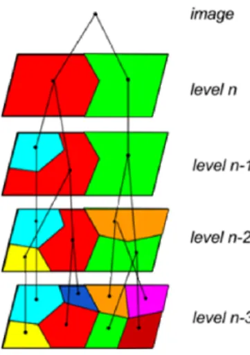
HSWO naturally produces a segmentation hierarchy consisting of the entire sequence of segmentations from initialization down to the final trivial one region segmentation (if allowed to proceed that far). For practical applications, however, a subset of segmentations needs to be selected out from this exhaustive segmentation hierarchy. At a minimum such a subset can be defined by storing the results only after a preselected number of regions is reached, and then storing selecting iterations after that such that no region is involved in more than one merge between stored iteration until a two region segmentation is reached. A portion of such a

segmentation hierarchy is illustrated in Figure 16-2. (The selection of a single segmentation from a segmentation hierarchy is discussed in Section 16.3.1.5.)

Figure 16-2. The last four levels of an n level segmentation hierarchy produced by a region growing segmentation process. Note that when depicted in this manner, the region growing process is a “bottom-up” approach.

A unique feature of the segmentation hierarchy produced by HSWO and related region growing segmentation approaches is that the segment or region boundaries are maintained at the full image spatial resolution for all levels of the segmentation hierarchy. The region boundaries are coarsened in many other multilevel representations.

Many variations on best merge region growing have been described in the literature. As early as 1994, Kurita (1994) described an implementation of the HSWO form of best merge region growing that utilized a heap data structure (Williams, 1964) for efficient determination of best merges and a dissimilarity criterion based on minimizing the mean squared error between the region mean image and original image. Further, several of the image segmentation

approaches studied in the previously referenced series of papers published by the Liebniz Institute are based on best merge region growing (see Table 16-1). As we will discuss in more detail later, the main differences between most of these region growing approaches are the

dissimilarity criterion employed and, perhaps, some control logic designed to remove small regions or otherwise tailor the segmentation output.

16.3.1.1. Seeded Region Growing

Seeded region growing is a variant on best merge region growing in which regions are grown from pre-selected seed pixels or seed regions. Adams and Bischof (1994) is an early example of this approach. In seeded region growing, the best merges are found by examining the pixels adjacent to each seed pixel of region formed around each seed pixel. As described by Adams and Bischof (1994), the region growing process continues until each image pixel is associated with one of the pre-selected seed pixels or regions.

16.3.1.2. Split and Merge Region Growing

In the split and merge approach, the image is repeatedly subdivided until each resulting region has a sufficiently high homogeneity. Examples of measures of homogeneity are the mean squared error between the region mean and the image data values, or the region standard

deviation. After the region-splitting process converges, the regions are grown using one of the previously described region growing approaches. This approach is more efficient when large homogeneous regions are present. However, some segmentation detail may be lost. See (Horowitz and Pavlidis, 1974), (Cross, et al., 1988), and (Strasters and Gerbrands, 1991) for examples of this approach.

16.3.1.3. Hybrid of Spectral Clustering and Region Growing

Tilton (1998) and Tilton, et al. (2012) describe a hybridization of HSWO best merge region growing with spectral clustering, called HSeg (for Hierarchical Segmentation). We remind the

reader that HSWO is performed by finding a threshold value, Tmerge, equal to the value of a

dissimilarity criterion of the most similar pair of spatially adjacent regions, and then merging all pairs of regions that have dissimilarity equal to Tmerge. HSeg adds to HSWO a step following

each step of adjacent region merges in which all pairs of spatially non-adjacent regions are merged that have dissimilarity <= SwTmerge, where 0.0 <= Sw <= 1.0 is a factor that sets the

priority between spatially adjacent and non-adjacent region merges. Note that when Sw = 0.0,

HSeg reduces to HSWO.

Unfortunately, the inclusion of the step in HSeg of merging spatially non-adjacent regions adds significantly to the computational requirements of this image segmentation approach. This is because comparisons must now be made between all pairs of regions instead of just between pairs of spatially adjacent regions. A recursive divide-and-conquer approach (called RHSeg), along with a parallel implementation, was developed to help overcome this problem (Tilton, 2007). The computational requirements of this approach were further reduced by a refinement in which the non-adjacent region merging was limited to between regions of a minimum size, Pmin

(Tilton, et al., 2012). In this refinement the value of Pmin is dynamically adjusted to keep the

number of “large regions” (those of at least Pmin in size) to a range that substantially reduces the

computational requirements without out significantly affecting the image segmentation results.

16.3.1.4. Dissimilarity Criterion and Specialized Control Logic

Muerle and Allen (1968) experimented with various criteria for determining whether or not pairs of region objects were similar enough to be merged together. They concluded that an optimal criterion would be a threshold of a function of the mean and standard deviation of the gray levels of the pixels contained in the compared region objects.

In our image segmentation research, we have implemented and studied several region merging criteria in the form of dissimilarity criteria (Tilton, 2013). Included among these dissimilarity criteria are criteria based on vector norms (the 1-, 2-, and ∞–norms), criteria based on minimizing the increase of mean squared error between the region mean image and the original image data, and a criterion based on the Spectral Angle Mapper (SAM) criterion (Kruse, et al., 1993). We briefly describe these dissimilarity criteria here.

The dissimilarity criterion based on the 1-Norm of the difference between the region mean vectors, ui and uj, of regions Xi and Xj, each with B spectral bands, is:

d1-Norm







where μib and μjb are the mean values for regions i and j, respectively, in spectral band b, i.e., ui =

(i1, i2, …, iB)T and uj = (j1, j2, …, jB)T.

The dissimilarity criterion based on the 2-Norm is:

d2-Norm









_

and the dissimilarity criterion based on the ∞-Norm is:

d-Norm









   (16-9)

As noted above, a criterion based on mean squared error minimizes the increase of mean squared error between the region mean image and the original image data as regions are grown. The sample estimate of the mean squared error for the segmentation of band b of the image X into R disjoint subsets X1, X2, , XR is given by:

 

 



 

_









X

MSE





is the mean squared error contribution for band b from segment Xi. Here, xp is a pixel vector (in

this case, a pixel vector in data subset Xi), and pb is the image data value for the bth spectral band

of the pixel vector, xp. The dissimilarity function based on a measure of the increase in mean

squared error due to the merge of regions Xi and Xj is given by:

dBSMSE











∆MSEb(Xi,Xj) = MSEb(Xi



BSMSE refers to “band sum MSE.” Using 10b) and exchanging the order of summation, (16-11b) can be manipulated to produce an efficient dissimilarity function based on aggregated region features (for the details, see (Tilton, 2013)):

dBSMSE















The dimensionality of the dBSMSE dissimilarity criteria is equal to the square of the dimensionality

of the image pixel values, while the dimensionality of the vector norm based dissimilarity criteria is equal to the dimensionality of the image pixel values. To keep the dissimilarity criteria

dimensionalities consistent, the square root of dBSMSE is often used.

The Spectral Angle Mapper (SAM) criterion is widely used in hyperspectral image analysis (Kruse, et al., 1993). This criterion determines the spectral similarity between two spectral vectors by calculating the “angle” between the two spectral vectors. An important property of the SAM criterion is that poorly illuminated and more brightly illuminated pixels of the same color

will be mapped to the same spectral angle despite the difference in illumination. The spectral angle  between the region mean vectors, ui and uj, of regions Xi and Xj is given by:











where μib and μjb are the mean values for regions i and j, respectively, in spectral band b, i.e., ui =

(i1, i2, …, iB)T and uj = (j1, j2, …, jB)T. The dissimilarity function for regions Xi and Xj,

based on the SAM distance vector measure, is given by:

dSAM



 



vectors.

A problem that can often occur with basic best merge region growing approaches is that the segmentation results contain many small regions. We have found this to be the case when employing dissimilarity criteria based on vector norms or SAM, but not a problem for

dissimilarity criteria based on minimizing the increase of mean squared error. This is because the mean squared error criterion has a factor, ⁄ − , where ni and nj are the number of

pixels in the two compared regions, that biases toward merging small regions into larger ones. We have found it useful to add on a similar “small region merge acceleration factor” to the vector norm and SAM based criterion when one of the compared regions is smaller than a certain size. See Tilton, et al. (2012) for more details.

Implementations of best merge region growing often add special control logic to reduce the number of small regions or otherwise improve the final classification result. An example of this is SEGEN (Gofman, 2006), which uses the vector 2-norm (otherwise known as Euclidean distance) for the dissimilarity criterion. As noted in Tilton, et al. (2012), SEGEN is a relatively pure implementation of best merge region growing, optimized for efficiency in performance, memory utilization, and image segmentation quality. SEGEN adds a number of (optional) procedures to best merge region growing, among them a low-pass filter to be applied on the first stage of the segmentation and outlier dispatching on the last stage. The latter removes outlier pixels and small segments by imbedding them in neighborhood segments with the smallest dissimilarity. SEGEN also provides several parameters to control the segmentation process. A set of “good in average” control values is suggested in (Gofman, 2006).

The best merge region growing segmentation approach employed in eCognition Developer utilizes a dissimilarity function that balances minimizing the increase of heterogeneity, f, in both color and shape (Baatz and Schape, 2000), (Benz, et al., 2004):

= ∙ ∆ℎ + ∙ ∆ℎ (16-14)

where wcolor and wshape are weights that range in value from 0 to 1 and must mutually sum up to

1.

The color component of heterogeneity, Δhcolor, is defined as follows:

∆ℎ = ∑ ∙ _, − ∙ _, + ∙ _, (16-15)

where nx is the number of pixels, with the subscript x=merge referring to the merged object, and

subscripts x = 1 or 2 referring to the first and second objects considered for merging. σc refers to

the standard deviation in channel (spectral band) c, with the same additional subscripting denoting the merged or pair of considered objects. wc is a channel weighting factor.

The shape component of heterogeneity, Δhshape, is defined as follows: ∆ℎ = ∙ ∆ℎ + ∙ ∆ℎ (16-16) where ∆ℎ = ∙ − ∙ √ + ∙√ (16-17) ∆ℎ = ∙ − ∙ + ∙ (16-18)

where l is the perimeter of the object, and b is the perimeter of the object’s bounding box. The weights wc, wcolor, wshape, wsmooth and wcompt can be selected to best suit a particular application.

The level of detail, or scale, of the segmentation is set by stopping the best merge region growing process when the increase if heterogeneity, f, for the best merge reaches a predefined threshold value. A multiresolution segmentation can be created by performing this process with a set of increasing thresholds.

In eCognition Developer, other segmentation procedures can be combined with the multiresolution approach. For example, spectral difference segmentation merges neighbor objects that fall within a user-defined maximum spectral difference. This procedure can be used to merge spectrally similar objects from the segmentation produced by the multiresolution approach.

16.3.1.5. Selection of a Single Segmentation from a Segmentation Hierarchy

Some best merge region growing approaches such as HSWO and HSeg do not produce a single segmentation result, but instead produce a segmentation hierarchy. The best merge region growing segmentation approach employed in eCognition Developer can also produce a

segmentation hierarchy. A segmentation hierarchy is a set of several image segmentations of the same image at different levels of detail in which the segmentations at coarser levels of detail can

be produced from simple merges of regions at finer levels of detail. In such a structure, an object of interest may be represented by multiple segments in finer levels of detail, and may be merged into a surrounding region at coarser levels of detail. A single segmentation level can be selected out of the segmentation hierarchy by analyzing the spatial and spectral characteristics of the individual regions, and by tracking the behavior of these characteristics throughout different levels of detail. A manual approach for doing this using a graphical user interface is described in (Tilton, 2003) and (Tilton, 2013). A preliminary study on automating this approach is described in (Plaza and Tilton, 2005) where it was proposed to automate this approach using joint

spectral/spatial homogeneity scores computed from segmented regions. An alternate approach for making spatially localized selections of segmentation detail based on matching region boundaries with edges produced by an edge detector is described in (Le Moigne and Tilton, 1995).

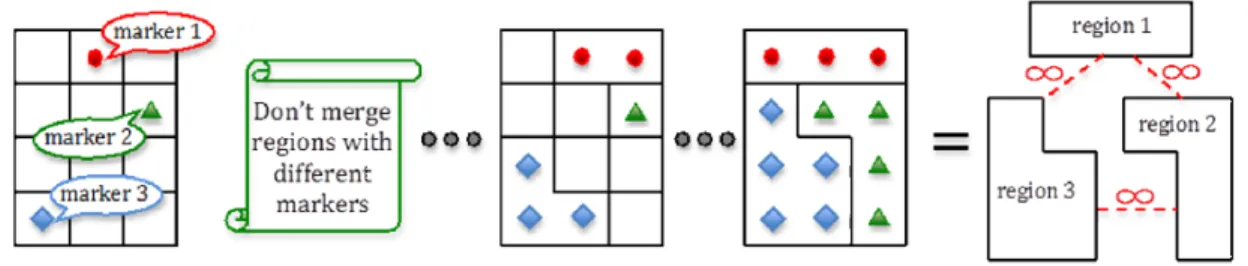
Tarabalka, et al. (2012) proposed a modification of HSeg through which a single

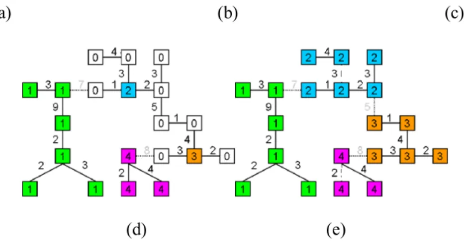
segmentation output is automatically selected for output from the usual segmentation hierarchy. The idea is similar to the previously described seeded region growing. The main idea behind the marker-based HSeg algorithm consists in automatically selecting seeds, or markers, for image regions, and then performing best merge region growing with an additional condition: two regions with different marker labels cannot be merged together (see Figure 16-3). The authors proposed to choose markers of spatial regions by analyzing results of a probabilistic supervised classification of each pixel and by retaining the most reliably classified pixels as region seeds.

Figure 16-3. Scheme illustrating the marker-based HSeg algorithm.

An alternative algorithm that produces a final segmentation by automatically selecting subsets of regions appearing in different levels in the segmentation hierarchy is described in Section 16.3.4.2

16.3.2. Texture-based Algorithms

Along with spectral information, textural features have also been heavily used for various image analysis tasks, including their use as features in thresholding-based, clustering-based, and region growing-based segmentation in the literature. In this section, we focus on the use of texture for unsupervised image segmentation. In the following, first, we discuss some particular examples that involve texture modeling for segmenting natural landscapes and man-made structures using local image properties, and then, present recent work on generalized texture algorithms that aim to model complex image structures in terms of the statistics and spatial arrangements of simpler image primitives.

One of the common uses of texture in remote sensing image analysis is the identification of natural landscapes. For example, Epifanio and Soille (2007) used morphological transformations such as white and black top-hat by reconstruction and thresholded image gradients with an unsupervised clustering procedure where the texture prototypes were automatically selected based on the dissimilarities between the feature vectors of neighboring image windows to segment vegetation zones and forest stands, and Wang and Boesch (2007) combined an initial

color-based oversegmentation step with a threshold-based region merging procedure that used wavelet feature statistics inside candidate image regions to delineate forest boundaries.

Man-made structures also exhibit particular characteristics that can be modeled using textural features. For example, Pesaresi, et al. (2008) proposed a rotation invariant anisotropic texture model that used contrast features computed from gray level co-occurrence matrices, and used this model to produce a built-up presence index. The motivation behind the use of the contrast-based features was to exploit the relationships between the buildings and their shadows. Sirmacek and Unsalan (2010) and Gueguen, et al. (2012) used a similar idea and modeled urban areas using spatial voting (smoothing) of local feature points extracted from the local maxima of Gabor filtering results and corner detection results, respectively. All of these results can be converted to a segmentation output by thresholding the corresponding urban area estimates.

An open problem in image segmentation is to identify the boundaries of regions that are not necessarily homogeneous with respect to low-level features such as color and texture that are extracted from individual pixels or from small local pixel neighborhoods. Recent literature includes several examples that can be considered as generalized texture algorithms that aim to model heterogeneous image content in terms of the spatial arrangements of relatively

homogeneous image primitives. Some of this work has considered the segmentation of particular structures that have specific textural properties. For example, Dogrusoz and Aksoy (2007) aimed the segmentation of regular and irregular urban structures by modeling the image content using a graph where building objects and the Voronoi tessellation of their locations formed the vertices and the edges, respectively, and the graph was clustered by thresholding its minimum spanning tree so that organized (formal) and unorganized (informal) settlement patterns were extracted to model urban development. Some agricultural structures such as permanent crops also exhibit

specific textural properties that can be useful for segmentation. For example, Aksoy, et al. (2012) proposed a texture model that is based on the idea that textures are made up of primitives (trees) appearing in a near-regular repetitive arrangement (planting patterns), and used this model to compute a regularity score for different scales and orientations by using projection profiles of multi-scale isotropic filter responses at multiple orientations. Then, they illustrated the use of this model for segmenting orchards by iteratively merging neighboring pixels that have similar regularity scores at similar scales and orientations.

More generic approaches have also been proposed for segmenting heterogeneous structures. For example, Gaetano, et al. (2009) started with an oversegmentation of atomic image regions, and then performed hierarchical texture segmentation by assuming that frequent neighboring regions are strongly related. These relations were represented using Markov chain models computed from quantized region labels, and the image regions that exhibit similar transition probabilities were clustered to construct a hierarchical set of segmentations. Zamalieva, et al. (2009) used a similar frequency-based approach by finding the significant relations between neighboring regions as the modes of a probability distribution estimated using the continuous features of region co-occurrences. Then, the resulting modes were used to construct the edges of a graph where a graph mining algorithm was used to find subgraphs that may correspond to atomic texture primitives that form the heterogeneous structures. The final segmentation was obtained by using the histograms of these subgraphs inside sliding windows centered at

individual pixels, and by clustering the pixels according to these histograms. As an alternative to graph-based grouping, Akcay, et al. (2010) performed Gaussian mixture-based clustering of the region co-occurrence features to identify frequent region pairs that are merged in each iteration of a hierarchical texture segmentation procedure.

In addition to using co-occurrence properties of neighboring regions to exploit statistical information, structural features can also be extracted to represent the spatial layout for texture modeling. For example, Akcay and Aksoy (2011) described a procedure for finding groups of aligned objects by performing a depth-first search on a graph representation of neighboring primitive objects. After the search procedure identified aligned groups of three or more objects that have centroids lying on a straight line with uniform spacing, an agglomerative hierarchical clustering algorithm was used to find larger groups of primitive objects that have similar spatial layouts. The approach was illustrated in the finding of groups of buildings that have different statistical and spatial characteristics that cannot be modeled using traditional segmentation methods. Another approach for modeling urban patterns using hierarchical segmentations

extracted from multiple images of the same scene at various resolutions was described by (Kurtz, et al., 2012) where binary partition trees were used to model image data and tree cuts were learned from user-defined segmentation examples for interactive partitioning of images into semantic heterogeneous regions.

16.3.3. Morphological Algorithms

Mathematical morphology has been successfully used for various tasks such as image

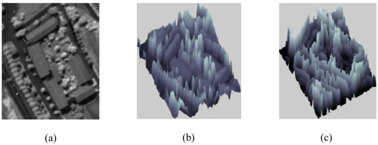
filtering for smoothing or enhancement, texture analysis, feature extraction, and detecting objects with certain shapes in the remote sensing literature (Soille and Pesaresi, 2002), (Soille, 2003). Morphological algorithms have also been one of the most widely used techniques for segmenting remotely sensed images. These approaches view the two-dimensional image data that consist of the spectral channels or some other property of the pixels as an imaginary topographic relief where higher pixel values map to higher imaginary elevation levels (see Figure 16-A). Consequently, differences in the elevations of the pixels in a spatial neighborhood can be

exploited to partition those pixels into different regions. Two morphological approaches for segmentation have found common use in the literature: watershed algorithms and morphological profiles. These approaches are described in the following sections. Other approaches using mathematical morphology for image segmentation, and particularly for producing segmentation hierarchies, can be found in (Soille, 2008), (Soille and Najman, 2010), (Ouzounis, et al., 2012), and (Perret, et al., 2012).

(a) (b) (c)

Figure 16-A. Illustration of mapping of the two-dimensional image data that consist of the spectral channels or some other property of the pixels as an imaginary topographic relief so that higher pixel values map to higher imaginary elevation levels. (a) An example spectral band. (b) The spectral values viewed as a three-dimensional topographic relief. (c) Gradient of the spectral data at each pixel viewed as a three-dimensional topographic relief.

16.3.3.1 Watershed Algorithms

The watershed algorithm divides the imaginary topographic relief into catchment basins so that each basin is associated with one local minimum in the image (i.e., individual segments) and the watershed lines correspond to the pixel locations that separate the catchment basins (i.e., segment boundaries). Watershed segmentation can be simulated by an immersion process

(Vincent and Soille, 1991). If we immerse the topographic surface in water, the water rises through the holes at the regional minima with a uniform rate. When two volumes of water coming from two different minima are about to merge, a dam is built at each point of contact. Following the immersion process, the union of all those dams constitutes the watershed lines. A graph-theoretical interpretation of the watershed algorithm can be found in (Meyer, 2001). Couprie, et al. (2011) describes a common framework that unifies watershed segmentation and some other graph-based segmentation algorithms that are described in Section 16.3.4.

The most commonly used method for constructing the topographic relief from the image data to be segmented is to use the gradient function at each pixel. This approach incorporates edge information in the segmentation process, and maps homogeneous image regions with low gradient values into the catchment basins and the pixels in high-contrast neighborhoods with high gradient values into the peaks in the elevation function. The gradient function for single-channel images can easily be computed using derivative filters. Multivariate extensions of the gradient function can be used to apply watershed segmentation to multispectral and hyperspectral images (Aptoula and Lefevre, 2007), (Noyel, et al., 2007), (Li and Xiao, 2007), and (Fauvel, et al., 2013).

A potential problem in the application of watershed segmentation to images with high levels of detail is oversegmentation when the watersheds are computed from raw image gradient where an individual segment is produced for each local minimum of the topographic relief.

Pre-processing or post-Pre-processing methods can be used to reduce oversegmentation. For example, smoothing filters such as the mean or median filters can be applied to the original image data as a pre-processing step. Alternatively, the oversegmentation produced by the watershed algorithm can be given as input to a region merging procedure for post-processing (Haris, et al., 1998).

Another commonly used alternative to reduce the oversegmentation is to use the concept of dynamics that are related to the regional minima of the image gradient. A regional minimum is composed of a group of neighboring pixels with the same value where the pixels on the external boundary of this group have a greater value. When we consider the image gradient as a

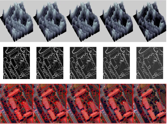
topographic surface, the dynamic of a regional minimum can be defined as the minimum height that a point in the minimum has to climb to reach a lower regional minimum (Najman and Schmitt, 1996). The ℎ-minima transform can be used to suppress the regional minima with dynamics less than or equal to a particular value ℎ by performing geodesic reconstruction by erosion of the input image from + ℎ (Soille, 2003). When it is difficult to select a single ℎ value, it is common to create a multi-scale segmentation by using an increasing sequence of ℎ values. The multi-scale watershed segmentation generates a set of nested partitions where the partition at scale is obtained as the watershed segmentation of the image gradient whose regional minima with dynamics less than or equal to are eliminated by using the ℎ-minima transform. First, the initial partition is calculated as the classical watershed corresponding to all local minima. Next, the two catchment basins having a dynamic of 1 are merged with their neighbor catchment basins at scale 1. Then, at each scale , the minima with dynamics less than or equal to are filtered whereas the minima with dynamics greater than remain the same or are extended. This continues until the last scale corresponding to the largest dynamic in the gradient image. Figure 16-B illustrates the use of the ℎ-minima transform for suppressing regional minima for obtaining a multi-scale watershed segmentation.

Figure 16-B. Illustration of the ℎ-minima transform for suppressing regional minima for obtaining a multi-scale watershed segmentation. The columns represent increasing values of ℎ, corresponding to decreasing amount of detail in the gradient data. The first row shows the gradient information at each pixel as a topographic relief. The second row shows the gradient data as an image. Brighter values represent higher gradient. The third row shows the

segmentation boundaries obtained by the watershed algorithm in red.

Yet another popular approach for computing the watershed segmentation without a significant amount of oversegmentation is to use markers (Meyer and Beucher, 1990). Marker controlled watershed segmentation can be defined as the watershed of an input image

transformed to have regional minima only at the marker locations. Possible methods for

identifying the markers include manual selection or selection of the pixels with high confidence values at the end of pixel-based supervised classification (Tarabalka, et al., 2010a). Given a marker image that consists of pixels whose value is 0 at the marker locations and a very large value in the rest of the image, the minima in the input image can be rearranged by using minima imposition. First, minima can be created only at the locations of the markers by taking the point-wise minimum between + 1 and . Note that the resulting image is lower than or equal to the marker image. The second step of the minima imposition is the morphological reconstruction by erosion of the resulting image from the marker image . Finally, watershed segmentation is applied to the resulting image. It is also possible to produce a multi-scale

segmentation by applying marker controlled watershed segmentation to the input image by using a decreasing set of markers. Marker selection is also discussed in Section 16.3.4.

16.3.3.2. Morphological Profiles

The image representation called morphological profiles was popularized in the remote sensing literature by Pesaresi and Benediktsson (2001). The representation uses the

morphological residuals between the original image function and the composition of a

granulometry constructed at multiple scales. The proposed approach makes use of both classical morphological operators such as opening and closing, and recent theoretical advances such as leveling and morphological spectrum to build the morphological profile.

The fundamental operators in mathematical morphology are erosion and dilation (Soille, 2003). Both of these operators use the definition of a pixel neighborhood with a particular shape called a structuring element (SE) (e.g., a disk of radius of 3 pixels). The erosion operator can be used to identify the image locations where the SE fits the objects in the image, and is defined as

the infimum of the values of the image function in the neighborhood defined by SE. The dilation operator can be used to identify the pixels where the SE hits the objects in the image, and is defined as the supremum of the image values in the neighborhood defined by SE. These two operators can be combined to define other operators. For example, the opening operator, which is defined as the result of erosion followed by dilation using the same SE, can be used to cut the peaks of the topographic relief that are smaller than the SE. On the other hand, the closing operator, which is defined as the result of dilation followed by erosion using the same SE, can be used to fill the valleys that are smaller than the SE.

The morphological operations are often used with the non-Euclidean geodesic metric instead of the classical Euclidean metric (Pesaresi and Benediktsson, 2001). The elementary geodesic dilation of (called the marker) under (called the mask) based on SE is the infimum of the elementary dilation of (with SE) and . Similarly, the elementary geodesic erosion of under

based on SE is the supremum of the elementary erosion of (with SE) and . A geodesic dilation (respectively, erosion) of size can also be obtained by performing successive elementary geodesic dilations (respectively, erosions). Next, the reconstruction by dilation (respectively, erosion) of under is obtained by the iterative use of an elementary geodesic dilation (respectively, erosion) of under until idempotence is achieved. Then, the opening by reconstruction of an image can be defined as the reconstruction by dilation of the erosion under the original image. Similarly, the closing by reconstruction of the image can be defined as the dual reconstruction by erosion of the dilation above the original image.

The advantage of the reconstruction filters is that they do not introduce discontinuities, and therefore, preserve the shapes observed in the input images. Hence, the opening and closing by reconstruction operators can be used to identify the sizes and shapes of different objects present

in the image such that opening (respectively, closing) by reconstruction preserves the shapes of the structures that are not removed by erosion (respectively, dilation), and the residual between the original image and the result of opening (respectively, closing) by reconstruction, called the top-hat (respectively, inverse top-hat, or bot-hat) transform, can be used to isolate the structures that are brighter (respectively, darker) than their surroundings.

However, to determine the shapes and sizes of all objects present in the image, it is necessary to use a range of different SE sizes. This concept is called granulometry. The morphological profile (MP) of size (2 + 1) can be defined as the composition of a

granulometry of size constructed with opening by reconstruction (opening profile), the original image, and an antigranulometry of size constructed with closing by reconstruction (closing profile) using a sequence of SEs with increasing sizes. Then, the derivative of the

morphological profile (DMP) is defined as a vector where the measure of the slope of the opening-closing profile is stored for every step of an increasing SE series (see Figures 16-C and 16-D for the illustration of opening and closing profiles, respectively).

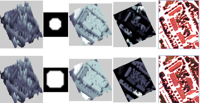
Figure 16-C. Illustration of the opening profile obtained using increasing SE sizes. Each row shows the results for an increasing SE series. The first column shows the input spectral data as a topographic relief. The second column shows the SEs used. The third column shows the result of opening by reconstruction of the topographic relief with the corresponding SEs. The fourth column shows the derivative of the opening morphological profile. The fifth column shows the boundaries of the connected components having a non-zero derivative profile for the

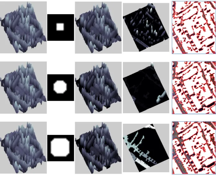
Figure 16-D. Illustration of the closing profile obtained using increasing SE sizes. Each row shows the results for an increasing SE series. The first column shows the input spectral data as a topographic relief. The second column shows the SEs used. The third column shows the result of closing by reconstruction of the topographic relief with the corresponding SEs. The fourth column shows the derivative of the closing morphological profile. The fifth column shows the boundaries of the connected components having a non-zero derivative profile for the

Pesaresi and Benediktsson (2001) used DMP for image segmentation. They defined the size of each pixel as the SE size at which the maximum derivative of the morphological profile is achieved. Then, they defined an image segment as a set of connected pixels showing the greatest value of the DMP for the same SE size. That is, the segment label of each pixel is assigned according to the scale corresponding to the largest derivative of its profile. This scheme works well in images where the structures are mostly flat so that all pixels in a structure have only one derivative maximum. A potential drawback of this scheme is that neighborhood information is not used at the final step of assigning segment labels to pixels. This may result in an

over-segmentation consisting of small noisy segments in very high spatial resolution images with non-flat structures where the scale with the largest value of the DMP may not correspond to the true structure.

Akcay and Aksoy (2008) proposed to consider the behavior of the neighbors of a pixel while assigning the segment label for that pixel. The method assumes that pixels with a positive DMP value at a particular SE size face a change with respect to their neighborhoods at that scale. As opposed to Pesaresi and Benediktsson (2001) where only the scale corresponding to the greatest DMP is used, the main idea is that a neighboring group of pixels that have a similar change for any particular SE size is a candidate segment for the final segmentation. These groups can be found by applying connected components analysis to the DMP at each scale. For each opening and closing profile, through increasing SE sizes from 1 to , each morphological operation reveals connected components that are contained within each other in a hierarchical manner where a pixel may be assigned to more than one connected component appearing at different SE sizes. Each component is treated as a candidate meaningful segment (see Figures C and 16-D). Using these segments, a tree is constructed where each connected component is a node and

there is an edge between two nodes corresponding to two consecutive scales if one node is contained within the other. Leaf nodes represent the components that appear for SE size 1. Root nodes represent the components that exist for SE size .

After forming a tree for each opening and closing profile, the goal is to search for the most meaningful connected components among those appearing at different scales in the segmentation hierarchy. Ideally, a meaningful segment is expected to be spectrally as homogeneous as

possible. However, in the extreme case, a single pixel is the most homogeneous. Hence, a segment is also desired to be as large as possible. In general, a segment stays almost the same (both in spectral homogeneity and size) for some number of SEs, and then faces a large change at a particular scale either because it merges with its surroundings to make a new structure or because it is completely lost. Consequently, the size of interest corresponds to the scale right before this change. In other words, if the nodes on a path in the tree stay homogeneous until some node , and then the homogeneity is lost in the next level, it can be said that corresponds to a meaningful segment in the hierarchy. With this motivation, to check the meaningfulness of a node, Akcay and Aksoy (2008) defined a measure consisting of two factors: spectral

homogeneity, which is calculated in terms of the difference of the standard deviation of the spectral features of the node and its parent, and neighborhood connectivity, which is calculated using sizes of connected components. Then, starting from the leaf nodes (level 1) up to the root node (level ), this measure is computed at each node, and a node is selected as a meaningful segment if it is highly homogeneous and large enough on its path in the hierarchy (a path corresponds to the set of nodes from a leaf to the root).

After the tree is finalized, each node is regarded as a candidate segment for the final segmentation. Given the goodness measure of each node in the hierarchy, the segments that

optimize this measure are selected by using a two-pass algorithm that satisfies the following conditions. Given as the set of all nodes and as the set of all paths in the tree, the algorithm selects ∗⊆ as the final segmentation such that any node in ∗ must have a measure greater than all of its descendants, any two nodes in ∗ cannot be on the same path (i.e., the

corresponding segments cannot overlap in the hierarchical segmentation), and every path must include a node that is in ∗ (i.e., the segmentation must cover the whole image). The first pass finds the nodes having a measure greater than all of their descendants in a bottom-up traversal. The second pass selects the most meaningful nodes having the largest measure on their

corresponding paths of the tree in a top-down traversal. The details of the algorithm can be found in (Akcay and Aksoy, 2008). Even though the algorithm was illustrated using a tree constructed from a DMP, it is a generic selection algorithm in the sense that it can be used with other

hierarchical image partitions, such as the ones described in Section 16.3.3, and can be applied to specific applications by defining different goodness measures for desired image segments (e.g., see (Genctav, et al., 2012) for an application of this selection algorithm to a hierarchical

segmentation produced by a multi-scale watershed procedure).

16.3.4. Graph-based Algorithms

Graph-based segmentation techniques gained popularity in recent years. In the graph-based framework, the image is modeled by a graph, where nodes typically represent individual pixels or regions, while edges connect spatially adjacent nodes. The weights of the edges reflect the (dis)similarity between the neighboring pixels/regions linked by the edge. The general idea is then to find subgraphs in this graph, which correspond to regions in the image scene. The early graph-theoretic approaches for image segmentation were described in (Zahn, 1971), where a minimum spanning tree was used to produce connected groups of vertices, and (Narendra, 1977),