A closed‐form solution to the asymptotic part of the MOM impedance matrix and the MOM excitation vector for printed structures on planar grounded dielectric slabs

(1)

inductors, and pads in silicon process, Ph.D. Thesis, National Central University, Taiwan, 2004.

6. Y.S. Lin and S.S. Lu, An analysis of the anomalous dip in scattering parameter S11 of InGaP/GaAs heterojunction bipolar transistors (HBTs), Jpn J Appl Phys B 43 (2004), L803–L805.

7. Y.S. Lin and S.S. Lu, An analysis of small-signal gate-drain resistance effect on RF power MOSFETs, IEEE Trans Electron Devices 50 (2003), 525–528.

8. H.Y. Tu, Y.S. Lin, P.Y. Chen, and S.S. Lu, An analysis of the anom-alous dip in scattering parameter S22of InGaP/GaAs heterojunction bipolar transistors (HBTs), IEEE Trans Electron Devices 49 (2002), 1831–1833.

9. S.S. Lu, C.C. Meng, T.W. Chen, and H.C. Chen, The origin of the kink phenomenon of transistor scattering parameter S22, IEEE Trans Micro-wave Theory Tech 49 (2001), 333–340.

A CLOSED-FORM SOLUTION TO THE

ASYMPTOTIC PART OF THE M

O

M

IMPEDANCE MATRIX AND THE M

O

M

EXCITATION VECTOR FOR PRINTED

STRUCTURES ON PLANAR GROUNDED

DIELECTRIC SLABS

O. Baky´r and V. B. Ertu¨rk

Department of Electrical and Electronics Engineering, Bilkent University, TR-06800, Bilkent, Ankara, Turkey

Received 18 August 2006

ABSTRACT: In the spectral domain method of moments (MoM) solu-tion of printed structures on planar grounded dielectric slabs, the infi-nite double integrals which appear in the asymptotic parts of the MoM impedance matrix and the MoM excitation vector elements, have been previously transformed to one-dimensional finite integrals, which have been numerically computed using the highly specialized “International Mathematics and Statistics Library” subroutines. In this paper, these one-dimensional integrals are evaluated in closed-form, resulting in an improved efficiency and accuracy for the rigorous investigation of printed antennas and complex millimeter and microwave integrated cir-cuits. Numerical results in the form of mutual impedance between two expansion functions and input impedance of various microstrip an-tennas are presented to assess the accuracy of these closed-form ex-pressions. © 2007 Wiley Periodicals, Inc. Microwave Opt Technol

Lett 49: 882– 886, 2007; Published online in Wiley InterScience (www. interscience.wiley.com). DOI 10.1002/mop.22274

Key words: method of moments; microstrip antennas; (M)MIC struc-tures; spectral domain analysis

1. INTRODUCTION

The spectral domain Method of Moments (MoM) solution to the integral equation is one of the widely used techniques for the analysis and design of printed antennas and arrays as well as microwave- and millimeter-wave integrated circuits due to its high accuracy and relatively good modeling capabilities [1–7]. In this technique, the elements in the MoM matrix equation are expressed as integrals over a spectrum of wave functions, rather than as integrals over the physical space of the expansion and weighting functions. Therefore, the impedance-matrix (and the MoM excita-tion vector in the case of probe-fed structures) elements are ex-pressed in terms of double integrals with limits extended to inﬁn-ity, which must be evaluated numerically. Unfortunately, the slowly convergent and highly oscillating behaviors of the

inte-grands make filling the impedance-matrix elements as the most time-consuming part in the MoM solution, in particular for elec-trically large structures. Besides, such behaviors may create accu-racy problems as well. Thus, various techniques have been devel-oped related to the spectral domain evaluation of the impedance matrix and the excitation vector entries [2–7]. Among them, in Refs. 5 and 6, the authors have successfully derived an analytical technique for the fast and accurate evaluation of the asymptotic part of the impedance matrix when triangular edge mode and roof-top subdomain basis functions are used in the spectral domain MoM solution for printed narrow strips and antennas. Basically, they provide an analytical transformation from an infinite double (2D) integral to a finite one-dimensional (1D) integral for the asymptotic part of the impedance matrix, thereby reducing the CPU time markedly and improving the accuracy regardless of the lateral separation between the basis and testing functions. Re-cently, the same method has been applied to the MoM excitation vector for probe-fed planar microstrip antennas [7].

In all these three studies [5–7], the resulting one-dimensional ﬁnite integrals are computed using the “International Mathematics and Statistics Library (IMSL)” subroutines DQDAGP (if there is a singularity) or DQDAGS, which are high-quality adaptive integral routines. Unfortunately, these routines are highly specialized and may not be available on all platforms. Moreover, using standard numerical integration techniques instead of these IMSL routines may yield accuracy problems. Therefore, in this paper we provide closed-form results for these 1D integrals. Consequently, the as-ymptotic parts of both the impedance matrix and the excitation vector are evaluated completely in closed-form, which results in a further reduction in the CPU time and a further improvement in the accuracy for the evaluation of the MoM matrix and the excitation vector entries. Besides, these closed-form expressions eliminate the need for such highly specialized subroutines for such problems. In Section 2, closed-form evaluation of the aforementioned 1D integrals is presented. In Section 3, numerical results involving the mutual impedance between two expansion functions and the input impedance of various microstrip antennas are calculated and com-pared with the published results to assess the accuracy of these closed-form expressions. An ejwt

time dependence is assumed and suppressed throughout this paper.

2. FORMULATION

In the spectral domain MoM solution of printed structures on planar grounded dielectric slabs, using Galerkin’s method and employing the asymptotic extraction technique, the impedance matrix elements can be expressed in the form of

Zmpq⬘n⬘mn⫽ ⫺ 1 4␲2

冕

⬁ ⬁

冕

⬁ ⬁ J˜mp*⬘n⬘共kx,ky兲 ⫻ 关G˜pq共kx,ky兲 ⫺ G˜pq⬁共kx,ky兲兴 J˜mn q 共kx,ky兲 dkxdky ⫺₄1_␲2

冕

⬁ ⬁

冕

⬁ ⬁ J˜mp*⬘n⬘共kx,ky兲G˜pq⬁共kx,ky兲J˜mn q 共kx,ky兲 dkxdky (1)

(p⫽ x or y, and q ⫽ x or y) where Zmpq⬘n⬘mnrepresents the self and

mutual interactions between the roof-top subdomain current basis functions Jmp⬘n⬘and Jmn

q _{. In Eq. (1), J˜} m⬘n⬘

p _{is the Fourier transform of}

the p-directed basis function (i.e., Jmp⬘n⬘), J˜mnq* is the complex

con-jugate of the Fourier transform of the q-directed basis function, and ﬁnally G˜pqis the appropriate dyadic Green’s function component

(2)

␤ ⫽

冑

kx2⫹ ky2values. The explicit expressions for Jmp⬘n⬘, its Fourier

transform, G˜_pqand G˜_pq⬁ _{are given in Ref. 6. In a similar fashion, the}

MoM excitation vector elements (for probe-fed structures) are expressed as Vmq⬘n⬘⫽ 1 4␲2

冕

⬁ ⬁

冕

⬁ ⬁ 关G˜zq共kx,ky兲 ⫺ G˜zq⬁共kx,ky兲兴J˜mq⬘n⬘共kx,ky兲 ⫻ ej共kxxp_⫹k_yyp_兲 dkxdky⫹ 1 4␲2

冕

⬁ ⬁

冕

⬁ ⬁ G˜_zq⬁_共k x,ky兲J˜m⬘n⬘ q 共kx,ky兲 ⫻ ej共kxxp_⫹k_yyp_兲 dkxdky (2) where (xp , yp

) is the coaxial probe attachment position on the patch surface and G˜zqis appropriate dyadic Green’s function component

in the spectral domain with G˜_zq⬁ _{being its asymptotic value for large}

␤ values. The explicit expressions for G˜zqand G˜zq⬁ are given in

Refs. 1 and 7.

ᑣb共␹兲, B共␹兲, T共␹ ⫺ xs兲, C共␹兲 and ⌫共␹ ⫺ xA兲 are given in Refs. 6

and 7. Basically, A共␹ ⫺ xs兲 is in Eqs. (39), (40), and (41), ᑣa共␹兲

in Eq. (26),ᑣb共␹兲 in Eq. (27), B共␹兲 in Eq. (45), and T共␹ ⫺ xs兲 in

Eq. (30) of Ref. 6, and C共␹兲 in Eq. (14) and ⌫共␹ ⫺ xA兲 in Eq. (11)

of Ref. 7, respectively. Similar expressions are formed for Imyy⬘n⬘mn

a

, Imyy⬘n⬘mn

b

, Imyx⬘n⬘mn, and Imzy⬘n⬘by interchanging⌬x 7 ⌬y, xs7 ysand xA

7 yA, where xsand ysare the lateral separation between the basis

and testing functions (i.e., xs⫽ xm⫺ xm⬘; ys⫽ yn⫺ yn⬘), xAand

yAare the separation between the basis function under analysis and

the probe location (i.e., xA⫽ xp⫺ xm⬘; yA⫽ yp⫺ yn⬘), and⌬x and

⌬y are related with the size of the roof-top functions as explained in Ref. 6 such that roof-top functions for the xˆ-directed current elements have dimensions 2⌬x and ⌬y in the xˆ and yˆ directions, respectively, while the size of roof-top for the yˆ-directed current elements have dimensions⌬x and 2⌬y in the xˆ and yˆ directions, respectively.

In Refs. 5–7, the 1D integrals given in Eqs. (3)–(6) were computed numerically using the IMSL subroutines. During the computation of these integrals, if there is a singularity at the integration interval, then the IMSL routine DQDAGP was used, which can handle interior and endpoint singularities. If there is no singularity, the IMSL routine DQDAGS was used. Unfortunately, these routines are highly specialized and may not be available on all platforms. Besides, it is observed that using standard numerical integration techniques instead of these IMSL routines yields ac-curacy problems. Therefore, in this study, we provide closed-form expressions for these integrals. The key steps in arriving at these closed-form expressions are

i. The analytic evaluation of the following type integrals:

共x ⫺ xs兲2⫹ a2兲 dx (10)

with i⫽ 0, 1, 2, 3. It is important to notice that Fi(a, x1, x2, xs) and

Gi(a, x1, x2, xs) are expressed in terms of fi(a, x1, x2) and gi(a, x1,

x₂), respectively.

ii. Recognizing that the closed-form expressions to the inte-grals given by Eqs. (3)–(6) can be obtained as a combina-tion of Eqs. (7)–(10).

Consequently, the closed-form expressions for the 1D integrals given by Eqs. (3)–(6) are found as follows:

p⫽1 3 兵dxy_{共q兲关c}xy_{共2p ⫺ 1兲共 f} 0共aq xy ,␹p xy ,␹pxy⫹1兲 ⫺ aq xy_G 0共aq xy ,␹p xy ,␹pxy⫹1兲兲 ⫹ cxy共2p兲共 f1共aq xy ,␹p xy ,␹pxy⫹1兲 ⫺ aq xy G1共aq xy ,␹p xy ,␹pxy⫹1兲兲其, (13) Imzx⬘n⬘⫽ G0共a1 zx ,␹1 zx ,␹2 zx_{兲 ⫺ G} 0共a2 zx ,␹1 zx ,␹2 zx_{兲 ⫺ G} 0共a1 zx ,␹2 zx ,␹3 zx_兲 ⫹ G0共a2 zx ,␹2 zx ,␹3 zx 兲. (14) In Eqs. (11) and (12), the constants and the coefﬁcients are given as follows: c₀s1⫽ 8⌬x3_{; c} 1 s1⫽ 12⌬x2_共⫺1兲q⫹1_{; c} 2 s1⫽ 6⌬x ; c 3 s1⫽ 共⫺1兲q⫹1_, (15) c₀s2⫽ ⫺4⌬x3_{; c} 1 s2⫽ 0 ; c 2 s2⫽ ⫺6⌬x ; c 3 s2⫽ 3共⫺1兲q , (16) c₀s3⫽ ⫺⌬x 4 ; c1 s3⫽1 8共⫺1兲 q ; c₀s4⫽⌬x 4 ; c1 s4⫽3 8共⫺1兲 q⫹1_, ₍₁₇₎ ␹1 xx ⫽ ⫺2⌬x ;␹2 xx ⫽ ⫺⌬x ;␹3 xx ⫽ 0 ;␹4 xx ⫽ ⌬x ;␹5 xx ⫽ 2⌬x, (18) a₁xx_{⫽ y} s⫹ ⌬y ; a2 xx_{⫽ y} s⫺ ⌬y ; a3 xx_{⫽ y} s, (19)

c_G共1兲 ⫽ ys⫹ ⌬y ; cG共2兲 ⫽ ys⫺ ⌬y ; cG共3兲 ⫽ ⫺2ys, (20)

cf共1兲 ⫽ ⫺1 ; cf共2兲 ⫽ ⫺1 ; cf共3兲 ⫽ 2. (21)

Similarly, in Eqs. (13) and (14), the constants and the coefﬁcients are as follows: ␹1 xy ⫽ ⫺1.5⌬x ⫹ xs;␹2 xy ⫽ ⫺0.5⌬x ⫹ xs;␹3 xy ⫽ 0.5⌬x ⫹ xs;␹4 xy_{⫽ 1.5⌬x ⫹ x} s, (22) a1 xy ⫽ ⫺1.5⌬y ⫹ ys; a2 xy ⫽ ⫺0.5⌬y ⫹ ys; a3 xy ⫽ 0.5⌬y ⫹ ys; a4 xy_{⫽ 1.5⌬y ⫹ y} s, (23) cxy_{共1兲 ⫽ ⫺}␲ 8共1.5⌬x ⫺ xs兲 ; c xy_{共2兲 ⫽ ⫺}␲ 8; c xy_{共3兲 ⫽ ⫺}␲ 4xs; cxy 共4兲 ⫽␲₄; cxy 共5兲 ⫽␲₈共1.5⌬x ⫹ xs兲 ; c xy 共6兲 ⫽ ⫺␲₈, (24) dxy 共1兲 ⫽ ⫺₁₆1 ; dxy 共2兲 ⫽₁₆3 ; dxy 共3兲 ⫽ ⫺₁₆3 ; dxy 共4兲 ⫽₁₆1, (25) ␹1 zx ⫽ xp⫺ ⌬x ;␹2 zx ⫽ xp;␹3 zx ⫽ xp⫹ ⌬x, (26) a₁zx ⫽ yp⫹ ⌬y 2 ;2 zx ⫽ yp⫺ ⌬y 2. (27)

Finally, the analytical expressions to the results of the integrals deﬁned in Eqs. (7)–(10), which are the main building blocks of Eqs. (11)–(14), are given by

, (30) f3共a, x1, x2兲 ⫽ 1 15共 x22⫹ a2兲3/ 2共3x22⫺ 2a2兲 ⫺₁₅1共 x12⫹ a2兲3/ 2共3x12⫺ 2a2兲, (31) F₀共a, x₁, x₂, xs兲 ⫽ f0共a, x1⫺ xs, x2⫺ xs兲, (32) F1共a, x1, x2, xs兲 ⫽ f1共a, x1⫺ xs, x2⫺ xs兲 ⫹ xsf0共a, x1⫺ xs, x2⫺ xs兲, (33)

F2共a, x1, x2, xs兲 ⫽ f2共a, x1⫺ xs, x2⫺ xs兲 ⫹ 2xsf1共a, x1⫺ xs, x2

⫺ xs兲 ⫹ xs 2_f

0共a, x1⫺ xs, x2⫺ xs兲, (34)

F3共a, x1, x2, xs兲 ⫽ f3共a, x1⫺ xs, x2⫺ xs兲 ⫹ 3xsf2共a, x1⫺ xs, x2

⫺ xs兲 ⫹ 3xs2f1共a, x1⫺ xs, x2⫺ xs兲 ⫹ xs3f0共a, x1⫺ xs, x2⫺ xs兲,

(35) G0共a, x1, x2兲 ⫽ 22ln共a ⫹

冑

x22⫹ a2兲 ⫺ x1ln共a ⫹

冑

x12⫹ a2兲

x1 2_{⫹ a}2_, ₍₃₉₎

(4)

G0共a, x1, x2, xs兲 ⫽ G0共a, x1⫺ x2⫺ xs兲, (40)

G1共a, x1, x2, xs兲 ⫽ G1共a, x1⫺ xs, x2⫺ xs兲

⫹ xsG0共a, x1⫺ xs, x2⫺ xs兲, (41)

G2共a, x1, x2, xs兲 ⫽ G2共a, x1⫺ xs, x2⫺ xs兲 ⫹ 2xsG1共a, x1⫺ xs, x2

⫺ xs兲 xs 2_G

0共a, x1⫺ xs, x2⫺ xs兲, (42)

G3共a, x1, x2, xs兲 ⫽ G3共a, x1⫺ xs, x2⫺ xs兲 ⫹ 3xsG2共a, x1⫺ xs, x2

⫺ xs兲 ⫹ 3xs2G1共a, x1⫺ xs, x2⫺ xs兲, ⫹ xs3G0共a, x1⫺ xs, x2⫺ xs兲.

(43)

3. NUMERICAL RESULTS AND DISCUSSION

To assess the accuracy of the closed-form expressions presented in Eqs. (11)–(14) with the related parameters given by Eqs. (15)–(43), several numerical results in the form of mutual impedance between two expansion functions and the input impedance of several probe-fed microstrip patch antennas are obtained and compared with the simu-lation and measurement results available in the literature.

The first numerical example is the duplication of Figure 2 in Ref. 6, where the finite 1D integrals are compared with the double infinite integrals using⌬x ⫽ ⌬y ⫽ 1 and ys⫽ 2⌬y for 0 ⱕ xsⱕ

10 for Eqs. (3) and (4), and using⌬x ⫽ ⌬y ⫽ 1 and ys⫽ 3/2⌬y

for 0ⱕ xsⱕ 10 for Eq. (5). We also evaluated the same integrals,

Eqs. (3)–(5), using the closed-form expressions. As depicted in Figure 1; excellent agreement is obtained.

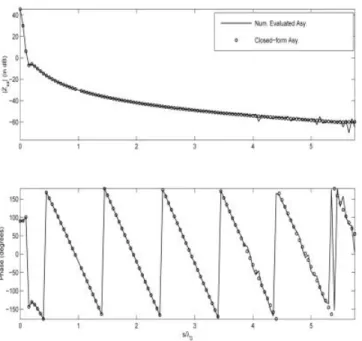
As a second example, the mutual interaction between two xˆ-directed current modes, which are deﬁned to be roof-top functions [Eq. (8) in Ref. 6], are evaluated along the H-plane (i.e., along the y-axis). These current modes are on a grounded dielectric slab with a thickness, h⫽ 0.057␭₀(␭₀is the free-space wavelength) and␧_r⫽ 2.33, and the size of each current mode is selected to be⌬x ⫽ 0.05␭₀ and⌬y ⫽ 0.025␭₀. Since IMSL routines are highly specialized and are not available on our platforms, we used the standard Gaussian quadrature algorithm in the following way: For the integration limits from⫺2⌬x to 2⌬x, we divided the integration interval to subintervals with the subinterval length being⌬x/8. In each subinterval we used an 8-point Gaussian quadrature algorithm. As seen in Figure 2, we have an excellent agreement both in magnitude and phase, except for relatively large separations, where the ﬁnite 1D integration method yields some numerical problems. As a result, we believe this result illustrates the importance of the closed-form expressions that we provide for the 1D integrals.

The last two numerical examples, shown in Figures 3 and 4, provide the Smith Chart plots of the input impedance of two probe-fed microstrip antennas, where the closed-form expressions for both the impedance matrix and the excitation vector are used. Results are also compared with the previously published results as well as the results of a software package ENSEMBLE [8]. Figure 3 is given for a rectangular microstrip patch antenna on a grounded dielectric slab with␧_r⫽ 10.2 and thickness h ⫽ 0.127 cm. The length of the patch L is 2 cm, the width of the patch W is 3 cm, and the feed is located 1 cm from the long edge (i.e., from the W edge) and 0.65 cm from the short edge (i.e., from the L edge) as explained in Ref. 9. The frequency is varied from 2.2 to 2.4 GHz, and 9 roof-top basis functions are used along the width of the patch. As seen in Figure 3, very good agreement is obtained with both the measured results given in Ref. 9 and the results obtained from the ENSEMBLE software [8].

In a similar fashion Figure 4 is given for W⫽ 39.52 mm by L ⫽ 49.91 mm rectangular antenna with a coaxial feed located at W/2

from the long side (i.e., from the L edge) and 15.36 mm from the short side (i.e., from the W edge) as depicted in Ref. 10. The antenna is located on a grounded dielectric slab with␧_r⫽ 2.484 and h⫽ 6.3 mm. The frequency is varied from 1.72 to 2.10 GHz, and ﬁve roof-top basis functions are used along the length of the patch. Similar to the previous case, very good agreement is ob-tained with both the measured and the simulated results given in Ref. 10 as well as the results obtained from the ENSEMBLE software [8]. Note that to account the self inductance of the probe we added jXprto the input impedance given by

Xpr⫽ ⫺

␩kh 2␲

冋

ln

冉

kd

4

冊

⫹ 0.577

册

(44) where␩ is the intrinsic impedance of the dielectric medium, k is the wave number of the dielectric medium, d is the diameter of the feed probe, and h is the thickness of the substrate [11].

4. CONCLUSIONS

Closed-form expressions are derived for the asymptotic parts of both the impedance matrix and the excitation vector of probe-fed printed geometries when spectral domain MoM solution is em-ployed. Previously, these asymptotic parts have been expressed as the ﬁnite 1D integrals that are computed using the IMSL

subrou-Figure 1 Comparison among the inﬁnite 2D integral, the ﬁnite 1D integral, and the closed-form expressions

(5)

tines DQDAGP and DQDAGS, which are highly specialized and may not be available on all platforms. Besides, it has been ob-served that using standard numerical integration techniques instead of these IMSL routines may yield accuracy problems. Conse-quently, implementation of these closed-form expressions to our existing spectral domain MoM codes eliminates the need for these specialized subroutines, and results in a further reduction in the CPU time and a further improvement in the accuracy for the evaluation of the MoM matrix and the excitation vector entries as illustrated in the numerical results in the form of mutual coupling

between two current modes and the input impedance of various probe-fed microstrip antennas.

ACKNOWLEDGMENTS

This work was supported in part by the Turkish Scientiﬁc and Technological Research Agency (TU¨ BI´TAK) under grant no EEEAG-104E044.

REFERENCES

1. D.M. Pozar, Input impedance and mutual coupling of rectangular micros-trip antennas, IEEE Trans Antennas Propagat 30 (1982), 1191–1196. 2. D.M. Pozar, Improved computational efﬁciency for the moment

method solution of printed dipoles and patches, Electromagnetics 3 (1983), 299 –309.

3. T. Vaupel and V. Hansen, Integral equation analysis of complex (M)MIC-structures with optimized system matrix decomposition and novel quadrature techniques, Adv Radio Sci 2 (2004), 101–105. 4. T. Vaupel, T.F. Eibert, and V. Hansen, Spectral domain analysis of

large (M)MIC-structures using novel quadrature methods, Int J Num Model: Electron Networks Devices Fields 18 (2005), 23–38. 5. S.-O. Park and C.A. Balanis, Analytical technique to evaluate the

asymptotic part of the impedance matrix of Sommerfeld-type integrals, IEEE Trans Antennas Propagat 45 (1997), 798 – 805.

6. S.-O. Park, C.A. Balanis, and C.R. Birtcher, Analytical evaluation of the asymptotic impedance matrix of a grounded dielectric slab with roof-top functions, IEEE Trans Antennas Propagat 46 (1998), 251–259. 7. F. Bilotti, A. Alu, F. Urbani, and L. Vegni, Asymptotic evaluation of

the MOM excitation vector for probe-fed microstrip antennas, J Elec-tromagn Waves Appl 19 (2005), 1639 –1654.

8. Ansoft Corporation, ENSEMBLE Version 8.0. www.ansoft.com, An-soft Corporation, Pittsburgh, PA.

9. D.H. Schaubert, D.M. Pozar, and A. Adrian, Effect of microstrip antenna substrate thickness and permittivity: comparison of theories with experiment. IEEE Trans Antennas Propagat 37 (1989), 677– 682. 10. R.C. Hall and J.R. Mosig, Rigorous feed model for coaxially fed

microstrip antenna, Electron Lett 26 (1990), 64 – 66.

11. C.A. Balanis, Antenna theory analysis and design, Wiley, New York, 1997.

Figure 2 Magnitude and phase variations of the mutual impedance Z12

xx

between two identical xˆ-directed current modes versus separation (s/␭0) on a h⫽ 0.057␭0thick grounded dielectric slab with␧r⫽ 2.33

Figure 3 Input impedance data of a probe-fed L⫽ 2 cm by W ⫽ 3 cm rectangular antenna on a h⫽ 0.127 cm thick grounded dielectric slab with ␧r⫽ 10.2. Frequency ⫽ 2.2–2.4 GHz

Figure 4 Input impedance data of a probe-fed L⫽ 49.91 mm by W ⫽ 39.52 mm rectangular antenna on a h⫽ 6.3 mm thick grounded dielectric slab with␧r⫽ 2.484. Frequency ⫽ 1.72–2.10 GHz