Influence function based Gaussianity tests for detection of microcalcifications in mammogram images

INFLUENCE FUNCTION BASED GAUSSIANITY TESTS FOR DETECTION OF

MICROCALCIFICATIONS IN MAMMOGRAM IMAGES

M. Nafi Gurcan', Yasemin Yardimci2, A. Enis Getin'

'

Department of Electrical and Electronics Engineering, Bilkent University, Ankara, Turkey

E-mail: cetin@ee.bilkent .edu.tr

Department of Computer Engineering, METU, Ankara, Turkey

ABSTRACT

In this paper, computer-aided diagnosis of microcal- cifications in mammogram images is considered. Mi- crocalcification clusters are an early sign of breast can- cer. Microcalcifications appear as single bright spots in mammogram images. We propose an effective method for the detection of these abnormalities. The first step of this method is two-dimensional adaptive filtering. The filtering produces an error image which is divided into overlapping square regions. In each square region, a Gaussianity test is applied. Since microcalcifications have an impulsive appearance, they are treated as out- liers. In regions with no microcalcifications, the dis- tribution of the error image is almost Gaussian, on the other hand, in regions containing microcalcifica- tion clusters, the distribution deviates from Gaussian- ity. Using the theory of the influence function and sen- sitivity curves, we develop a Gaussianity test. Micro- calcification clusters are detected using the Gaussianity test. Computer simulation studies are presented.

1. INTRODUCTION

Breast cancer is one of the most deadly diseases for women. The survival rate approaches 100 percent if cancer is detected early. Microcalcifications are an early sign of breast cancer and they appear as sin- gle, bright spots on mammograms (X-ray images of breasts). Because they are small and subtle, microcal- cifications are difficult t o detect by radiologists. In this work, we develop a computer-aided diagnosis (CAD) scheme for the detection of microcalcification clusters. Recently, we developed CAD schemes for the com- puterized detection of microcalcifications based on higher order statistics, adaptive filtering and Gaussian- ity tests [l, 2, 31. In these schemes, we make use of two- dimensional (2-D) adaptive filtering and a Gaussianity test recently developed by Ojeda et al. (the OCM test

for short) for causal invertible time series [4].

In our method, a Least Mean Square (LMS) type 2-D adaptive filter is used. The adaptive filter predicts an image pixel x[m, n] at location ( m , n) as a weighted average of pixels in its region of support. The region of support,

R,

of the filter is chosen as the pixels sur- rounding the pixel to be predicted. The predicted value ?[m, n] is given as

IC=-n1 Z=-n2

( I C 7 0

#

(0,O)

m=O , . . . , N l - - l , n=O

,...,

N 2 - 1 (1) where x is the input image of size NI x N2, w ( ~ , ~ ) are the weight values at ( m , n ) , and (2n1

+

1) x (2n2

+

1) is the size of the region of support, R of the adaptive filter.

The prediction error at pixel location ( m , n ) is com- puted as the difference between the predicted pixel value, i[m, n], and the actual pixel value, z [ m , n]

e[m, n] = i[m, n] - z [ m , n] ₍₂₎ At each iteration the weights w ( ~ , ~ ) [IC, Z] are adapted using a two-dimensional LMS-type adaptation algo- rithm:

w(m+l,n)

[IC,

11 = W(m,n) [IC, 11

+

P x e[m,

.I

x ~ [ k , 11 (3) where (IC,Z) E R, the region of support, and p is the adaptation constant.

Since microcalcifications are isolated bright spots, the prediction error sequence deviates from Gaussian- ity around microcalcification locations. Therefore, a statistics of the prediction errors is computed to deter- mine whether they are samples from a Gaussian distri- bution. The regions with Gaussianity test values higher

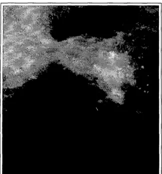
Figure 1: Part of a mammogram image which contains a microcalcification cluster.

than a set threshold value, Th, are marked as regions of microcalcification clusters. Figure 1 shows part of a mammogram image containing a microcalcification cluster. In Figure 2, the detection scheme output is given.

The contribution of this paper is twofold: we pro- pose an alternative Gaussianity test to the OCM Gaus- sianity test. We proceed by computing the sensi- tivity curves for the two techniques. The sensitivity curves indicate that our test is more sensitive to out- liers therefore it provides higher microcalcification de- tection rates. The results are validated by computer simulation studies. In the following section, the OCM Gaussianity test is reviewed. Section 4 describes the design of a new Gaussianity test based on the sensitiv- ity curve concept reviewed in Section 3. Results and conclusions are given in Section 5 .

2 . THE OCM GAUSSIANITY TEST

The OCM Gaussianity test is based on the sample es- timates of the first three moments I1,12,13 of the pre- diction errors. Estimates of the moments are given by:

Figure 2: Detection scheme output. Regions with mi- crocalcifications are indicated by the detection scheme.

where, e[m,n]’s ( m = 1,.

. .

,

M , n = 1 , .

.

.

,

N ) are in-

dividual error values at the location (m, n ) after adap-

tive filtering and M x N is the total number of error pixels in the square region ( M = N = 30 in our exper- iments). For Gaussian distributed sequences, I1,12,13 converge to the following values as M , N go to infinity under the ergodicity assumption

I1

+

p , I2

+

cr2

+

p 2 , p 3

+

3 a 2 p (5) where p and cr2 denote the mean and the variance of the error sequence e , respectively. With these limit values, the nonlinear expression

is close t o zero for Gaussian distributed sequences. Otherwise, it is concluded that the sequence deviates from Gaussianity. In the following section we estimate the sensitivity of this Gaussianity test t o outliers.

3. SENSITIVITY ANALYSIS

The sensitivity analysis of Gaussianity tests are based on sensitivity curve which is a finite-sample version of the influence function. The Influence Function (IF) of an estimator, T, for the cumulative distribution, F , is

given by [6]:

(7) T((1- t ) F

+

6 x )

-

T ( F )

I F ( x ; T , F ) = lim

t+O t

where 6x is the probability measure which puts mass 1

at point x . The influence function describes the effect

of an infinitesimal contamination at the point x on the estimate. The influence function for the sample mean function, T,, =

Cy=1

x i , for the Gaussian distributed

sequences is I F ( x ; T , F ) = x .

Tukey derived a simple finite-sample version of Equa- tion 7 [7]:

SC, = n [ T , ( x l ,

. . .

,

~ ~ -x ) 1

-

, Tn-l ( 2 1

,

. . .

,

x n - l ) ] ( 8 )

This is called the sensitivity curve which basically ex- amines the effect of an additional term, x as an out- lier on the overall estimator. First, the estimator value, Tn-l ( 5 1 ,

. . .

,

x,,-1) for n

-

1 terms is calculated.

Next, the outlier term, x is added to the sequence

and the estimator is again calculated for the n terms,

T , , ( z l , .

. .

,

x,-1, x ) . The difference between these two

estimator values exhibits the effect of the outlier on the estimator. The sensitivity curve, S n ( x ) , can be plotted

against values of the outlier, x to visualize the effect of

different values of outliers on the the overall sensitivity of the estimator (see Figure 3 ) .

The Gaussianity test in Equation 6 can be simplified to obtain the following expression:

h(11,12,13) = 13 - 31112

+

21: ₍₉₎

The overall sensitivity of the Gaussianity test

h(11,12,13) can be calculated by calculating S C n ( x )

values for 1 3 , 1 1 1 2 , 1: and then combining the results. So, the overall sensitivity curve is

+

x

(

--+-

Z2)

where cp := X I

+.

.

. + x n - l , and R := x:

+.

.

. + x i - l .

For Gaussian sequences and for large values of the sample size, n

cp R

- n

+

P ,

;

+

(/A2

+

2 )

where p is the mean and U is the standard deviation.

Substituting these values into Equation 10, we get

3

SCn(X) = x3 (1

-;

+

$)

I x

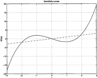
Figure 3: Sensitivity curves for the mean (dashed lines)

and for the Gaussianity test in Equation 9 (solid line)

+

x ’ n p ( - ; + $ ) 3 n

For Gaussian sequences with zero mean and standard deviation of one, Equation 12 further simplifies to:

SCn(X) = x3 (1 -

;

3

+

$)

-

32 ₍₁₃₎

For large values of n (i.e., n

+

oo), the sensitivity curve is reduced to

SCn(X) = x3 - 3x ₍₁₄₎

If we choose 2 1 , .

. .

,

x,-1 as 900 random Gaussian dis-

tributed numbers with zero mean and standard devia- tion of one, then the sensitivity curve in Figure 3 is ob-

tained. This curve closely fits t o the curve y = x3 - 32

as can be expected from Equation 12.

It is possible to design other Gaussianity tests, which makes use of higher order moments in order to have higher sensitivities. This will be useful in the detection of microcalcifications as they will be treated as outliers and more sensitive tests will be able to detect them with more ease.

4. FOURTH ORDER GAUSSIANITY TEST

Traditionally, both third and fourth order statistical parameters are used in Gaussianity detection. In the OCM test, parameters up t o the third order are used. By introducing the fourth order, the sensitivity of the

statistical test to outliers can be improved. Since mi- crocalcifications will produce outliers in the error im- age and tests with higher sensitivities can detect the outliers better, the higher the sensitivity of the Gaus- sianity test, the better its microcalcification detection performance is.

The fourth order moment is derived from the mo- ment generating function, M x ( t ) , of the Gaussian dis- tribution [8]

The kth order moment of distribution,

4 ,

is defined in terms of the moment generating function as follows

Of particular interest here is the fourth moment which is obtained using the following relation:

1 4 =

+

t 2 ( 6 a 6 [p4

+

3u4

+

6 p 2 a 4 )

+

6 p 2 a 2

+

t 3 ( p a 6

+

t(12pua4

+

3 p a 6 )

+

4 p 3 0 2 )

+ t 4 a 8 ] e t p + ~ 2 t 2 / 2 (17)

In the limit, when the value o f t is taken as zero, only the first three terms remain in the above expression and these constitute the fourth moment, 1 4 . Hence,

1 4 = E ( x 4 ) = p4

+

6 p 2 a 2

+

3a4 ₍₁₈₎

In designing the test, we want to establish a function such that it will assume the value of zero for Gaussian distributed sequences. First, a term is needed t o elim- inate the p4 term. In the limit, the moment 11 ap- proaches to the value of p , therefore, the fourth power of this moment can be subtracted from the fourth mo- ment term, 4 . In the limit, ( 1 2 -1;) approaches t o a 2 ,

which can then be used to eliminate the second and third terms of the moment expression. Therefore, the statistic for the Gaussianity test turns out to be:

which can be then simplified by eliminating the repetitive terms to get:

x

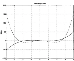
Figure 4: Sensitivity curves for the Gaussianity test in Equation 9 (solid line) and for the Gaussianity test in Equation 20 (dashed line).

The overall sensitivity curve of the new test is: SCn(X) = x 4 ( l - ; + - 3 + x 3 4 3 3

+

x 2 ( S V 2

-

!cl)

+

x ( - $ ) ( 2 1 )

As n -+ 00,

becomes:

-+ /I,

E

-+ (a2

+

p'), Equation 21

which boils down

to

the following relation for Gaussian signals with zero mean and the standard deviation of one:

S C n ( x ) = x4

-

6 x 2 _{( 2 3 )}

So, the overall sensitivity of the newly developed Gaussianity test is higher than that of Equation 9. As

a natural extension, other Gaussianity tests which use moments higher than fourth order moments can be de- signed. However, these moments converge very slowly to the normal distributions and so should not be used unless very large samples are processed [5].

I

Test Statistic

1

Mean

I Minimum

I

Maximum

1

h(11,12,13)

H(I1, I z , 1 4 )

38.6 8.4 306.0

406.8 52.4 3712.3

Table 1: Test statistics in regions with microcalcifica- tions.

h(11,12,13)

H(I1,

I?,

14)

I

Test Statistic

I

Mean

I

Minimum

I

Maximum

I

0.4 -2.1 2.2

1.25 -4.4 11.1

Table 2: Test statistics in regions without microcalcifi- cations.

5. RESULTS AND CONCLUSIONS

When the new Gaussianity test is used with the adap- tive filtering scheme, the statistics in Tables 1 and 2 are obtained. The test results are obtained from 100 differ- ent regions on 5 different mammogram images. With this test, the effect of outliers is more apparent. Fig- ure 4 shows this effect. Since the microcalcifications appear as outliers, they will be more pronounced with this test. Actually, the values of the newly developed test in Equation 20, reflect this change, while the val- ues in regions with no microcalcifications remain close to zero, in regions with microcalcifications, both Gaus- sianity tests produce high test statistics values. The fourth order Gaussianity test gives higher values than the OCM Gaussianity test.

As the range between the maximum value of one region and the minimum value of the other region is larger, it is possible t o set the detection threshold,

Th, at a higher level and eliminate some of the false

alarms (or single-bright spot regions). We tested the effectiveness of our new Gaussianity test using the Ni- jmegen mammogram image database’. The database contains 40 digitized mammogram images. Using only the OCM test in our previous detection scheme we were able to get 1.4 false alarm regions per image when all the radiologist-approved microcalcification clusters were detected [l]. When the newly developed Gaus- sianity test is used in combination with the OCM Gaus- sianity test, the false alarm rate decreases from 1.4 per image to 1.125 per image.

6. REFERENCES

[l] M. Nafi Gurcan, Yasemin Yardimci, A. Enis Cetin, ‘‘Microcalcification Detection Using Adaptive Fil- tering and Gaussianity Tests,” Proceedings of the Fourth International Workshop on Digital Mam- mography, pp. 157-164, June 1998, Nijmegen, The Netherlands.

I

[2] Metin Nafi Gurcan, Y. Yardimci, A. E. Cetin, “2-D Adaptive Filtering Based Gaussianity Tests in Microcalcification Detection,” Proceedings of SPIE Visual Communications and Image Process- ing Conference, vol. 3309, part 11, pp. 625- 633, 24-30 January, 1998, San Jose, CA.

[3] M. Nafi Giircan, Yasemin Yardimci, A. Enis Cetin, Rashid Ansari, “Detection of Microcalcifications in Mammograms Using Higher Order Statistics,” IEEE Signal Processing Letters, vol. 4, no. 8, pp 213-216, August 1997.

[4] R. Ojeda, J. Cardoso, E. Moulines, “Asymptoti- cally Invariant Gaussianity Test For Causal Invert- ible Time Series,” Proceedings of IEEE Interna- tional Conference on Acoustics, Speech, and Sig- nal Processing, vol. 5, pp. 3713-3716, April 21-24, 1997.

[5] E. Moulines, K. Choukri, “Time-Domain Proce- dures for Testing that a Stationary Time-Series is Gaussian,” IEEE Transactions on Signal Process- ing, vol. 44, no. 8, pp. 2010-2025, August 1996. [6] F. R. Hampel, E. M. Ronchetti, P. J. Rousseeuw,

W. A. Stahel, Robust Statistics: The Approach Based on the Influence Functions, John Wiley & Sons, New York : 1986.

[7] J. W. Tukey, Explaratory Data Analysis, Addison- Wesley, Reading, Mass. : 1971.

[8] W. W. Hines and D. C. Montgomery, Probabil- ity and Statistics in Engineering and Management Science, John Wiley and Sons, New York : 1980.

‘Images were provided by courtesy of the National Expert and Training Centre for Breast Cancer Screening and the Department of Radiology at the University of Nijmegen, the Netherlands.