Where have all the solar-like stars gone? Rotation period detectability at various inclinations and metallicities
Timo Reinhold,1 Alexander I. Shapiro,1 Veronika Witzke,1 Nina-E. N`emec,1, 2 Emre Is¸ık,3 and Sami K. Solanki1, 4
1Max-Planck-Institut f¨ur Sonnensystemforschung Justus-von-Liebig-Weg 3, 37077 G¨ottingen, Germany
2Institut f¨ur Astrophysik, Georg-August-Universit¨at G¨ottingen, Friedrich-Hund-Platz 1, D-37077 G¨ottingen, Germany
3Dept. of Computer Science, Turkish-German University S¸ahinkaya Cd. 108, Beykoz, 34820 Istanbul, Turkey 4School of Space Research, Kyung Hee University,
Yongin, Gyeonggi, 446-701, Korea
(Received; Revised; Accepted)
Submitted to ApJL ABSTRACT
The plethora of photometric data collected by the Kepler space telescope has pro-moted the detection of tens of thousands of stellar rotation periods. However, these periods are not found to an equal extent among different spectral types. Interest-ingly, early G-type stars with near-solar rotation periods are strongly underrepre-sented among those stars with known rotation periods. In this study we investigate whether the small number of such stars can be explained by difficulties in the period determination from photometric time series. For that purpose, we generate model light curves of early G-type stars with solar rotation periods for different inclination angles, metallicities and (magnitudependent) noise levels. We find that the de-tectability is determined by the predominant type of activity (i.e. spot or faculae domination) on the surface, which defines the degree of irregularity of the light curve, and further depends on the level of photometric noise. These two effects significantly complicate the period detection and explain the lack of solar-like stars with known near-solar rotation periods. We conclude that the rotation periods of the majority of solar-like stars with near-solar rotation periods remain undetected to date. Finally, we promote the use of new techniques to recover more periods of near-solar rotators.
1. INTRODUCTION
Corresponding author: Timo Reinhold
Stellar brightness variations at the timescale of stellar rotation are caused by transits of magnetic features (such as dark spots or bright faculae) rotating across the visible disk. These variations have routinely been observed by transit photometry missions. In particular, the Kepler telescope obtained light curves of roughly 150,000 main-sequence stars. Some of these light curves exhibit clear signatures of stellar rotation, which can be extracted by standard frequency analysis tools such as Lomb-Scargle periodograms, auto-correlation functions, or wavelet transforms. The biggest survey of rotation periods based on the Kepler data has been published by McQuillan et al. 2014(hereafterMMA14), who detected rotation periods for 34,030 presumably main-sequence stars.
However, for the majority of the main-sequence stars the light curves were either too noisy or too irregular for the rotation period to be determined. MMA14 found that the fraction of stars with detectable periods strongly depends on the effective temperature. Interestingly, this fraction appeared to be lowest for stars with near-solar effective temperature (between 5500–6000 K, hereafter referred to as early G-type stars), reaching only 16% (see Table 3 in MMA14). On the contrary, van Saders et al.(2019) used Galactic evolution models to predict that ∼59% of the early G-type stars should have detectable rotation periods.
The lack of stars with known rotation period becomes even more severe for early G-type stars of near-solar age. Recently, Reinhold et al. (2020) showed that only a dozen Kepler stars with near-solar fundamental parameters and rotation periods between 20–30 days (i.e. encompassing the solar rotation period of ∼25 days) exhibit rotational variability levels similar to that of the Sun. In contrast, the majority of these stars are substantially more variable than the Sun and also show more regular light curves patterns. It has been proposed that such a conspicuous difference between the Sun and other solar-like stars can be explained by a detection bias towards more active stars in bulk rotation period measurements (see the discussion inAmazo-G´omez et al. 2020), thus missing the majority of early G-type stars with near-solar rotation periods and small variabilities.
In this Letter we address the question whether the ”missing” solar-like stars (i.e. stars with solar fundamental parameters and rotation periods) do not exist or sim-ply go undetected. Our approach is based on the solar paradigm, i.e. we build on the comprehensive understanding of solar brightness variability (see, e.g., reviews by
Ermolli et al. 2013; Solanki et al. 2013), and extend solar models to solar-like stars. Namely, we combine two recently developed physics-based models by Witzke et al.
(2020) and N`emec et al. (2020). This allows calculating light curves of stars with a solar distribution of active regions and solar effective temperature, but various metal-licities and observed at arbitrary inclination angles. These light curves are used to identify obstacles in the period determination of solar-like stars, and to discuss pos-sible limitations of period measurements in real data sets. We further compare the
number of actual period measurements in Kepler data to predictions from Galactic evolution models using the detection rate obtained from the model light curves.
2. METHODS
2.1. The curious case of the Sun
The morphology of the solar light curve (as it would be observed in the Total Solar Irradiance or in the broad-band spectral passband like those of CoRoT, Kepler, or TESS) changes significantly depending on the phase of the solar activity cycle. While it appears to be quite regular at 11-year cycle minima when activity is low, the regularity disappears at periods of intermediate and high solar activity (Lanza & Shkolnik 2014; Aigrain et al. 2015; He et al. 2015). In particular, Amazo-G´omez et al.(2020) showed that if the Sun were observed by Kepler, the standard frequency analysis tools would most probably fail to detect the correct rotation period (unless observations are done during epochs of low solar activity). The causes for this inability are manifold: solar rotational variability is mainly brought about by spots (see, e.g.,
Shapiro et al. 2016). The relatively short lifetimes of sunspots from days to weeks (see, e.g., Solanki 2003) implies that most of the spots transit the visible solar disk only once, which leads to irregularities in the solar light curve, and hampers the detection of the solar rotation period. Furthermore, the brightness changes of dark spots and bright faculae partly compensate each other, which decreases the amplitude of the rotational signal, further hindering the period determination (Shapiro et al. 2017;
Witzke et al. 2020;N`emec et al. 2020). The exception from this general tendency are epochs of low solar activity with a small number of active regions. At these times the rotational variability is attributed to long-lived facular features and the light curve pattern becomes more periodic.
2.2. The model
While the irregularity of the solar light curve is quite well understood, the situation gets more complicated for other early G-type stars. Their light curves look different, partly because the stars are observed at various inclinations. For example, faculae appear brighter at the limb and therefore contribute more strongly to the variability when the star is observed out of the ecliptic plane (N`emec et al. 2020). Addition-ally, stellar metallicity [Fe/H] affects facular (and to a smaller degree spot) contrasts (Witzke et al. 2018), which eventually has an impact on the period detectability (Witzke et al. 2020).
To synthesize the light curves of solar-like stars, we built on recent calculations by N`emec et al. (2020) and by Witzke et al. (2018). N`emec et al. (2020) utilized a semi-empirical sunspot-group record by Jiang et al. (2011) and the Surface Flux Transport Model by Cameron et al. (2010) to reconstruct the distribution of active regions on the solar surface from the year 2010 back to 1700 with a daily cadence. By applying an appropriate geometrical transformation, N`emec et al. (2020) calculated the distribution of active regions on the solar disk as it would be observed at arbitrary
inclinations. Witzke et al. (2018) calculated the brightness contrasts of faculae and spots relative to the quiet Sun (i.e. free from any apparent manifestations of magnetic activity) as a function of wavelength and position on the visible disk for stars with different metallicities and solar effective temperature.
All in all, by combining the reconstructed disk distribution of active regions with their brightness contrasts, we generated light curves with a time span of 310 years as they would be seen in the passband of the Kepler telescope. The light curves were calculated for ten inclination angles 0◦ ≤ i ≤ 90◦ (with a step of 10◦), and
nine different metallicities −0.4 ≤ [Fe/H] ≤ 0.4 dex (with a step of 0.1 dex). The solar record from 1700–2010 covers epochs of both low solar activity (like the Dalton minimum around 1790–1830), and very high solar activity (like the modern grand maximum around 1950–2000, see Solanki et al. 2004; Usoskin et al. 2007), which allows studying rotation period detectability during activity cycles of very different strengths. We note that, by assuming a solar disk distribution of active regions, we only account for the metallicity effect on the contrasts of magnetic features. A change in metallicity also affects the depth of the convective zone, which in turn could influence the stellar dynamo, in particular the length of the stellar activity cycle or the emergence latitudes of magnetic bipoles (Schuessler & Solanki 1992). However, this effects is rather weak, e.g. doubling the metallicity of a star with solar temperature will deepen the convective zone by only ca. 8% (van Saders & Pinsonneault 2012;
Karoff et al. 2018). Therefore, we expect these effects to be relatively small. Studying them is beyond the scope of the present paper, but would be an interesting future exercise.
2.3. Monte Carlo approach
We take a Monte Carlo approach to analyze light curves with different realizations of inclination angles and metallicities. The distribution of inclination angles is uniform in cos i, where i = 0◦ denotes a pole-on view and i = 90◦ an equator-on view. The input distribution of metallicities was adapted for solar-like stars in the Kepler field (see Fig. A.1 and Reinhold et al. 2020). For each (random) parameter combination (i, [Fe/H]), we chose the model light curve from the grid with the closest parameters in metallicity and inclination angle.
Following the observing strategy of the Kepler telescope, we pick a random 4-year segment of the full time series (see top row of Fig.1for example). This light curve is then cut into 90-day segments (i.e. similar to the Kepler observing quarters), where each 90-day chunk is normalized by its median, and appended to the previous one, to form a 4-year time series. These Keplerized light curves (Fig. 1, middle row) will be analyzed for rotation in the next step. The detrending is necessary because it filters out brightness variations on the activity-cycle timescale, and renders the light curves comparable to detrended Kepler data.
In addition to the various inclination and metallicity combinations, we study the impact of noise on the period detectability. The model light curves are by definition noise-free. In real observations, the visual stellar magnitude defines the noise level. We use the distribution of Kepler magnitudes Kp of solar-like stars to compute dif-ferent noise realizations σ (see Reinhold et al. 2020 for details). A noise time series with zero mean and standard deviation σ is then added to the time series in the Monte-Carlo simulation. In total, we conducted 50,000 Monte Carlo runs, both for the noise-free and the noisy cases to study them separately.
3. RESULTS 3.1. Period detection
From among the various period detection methods, we chose the auto-correlation function (ACF) to search for periodicity in the time series (i.e. the same method as employed byMMA14). The ACF returns peaks of different power as a measure of the periodicity in the light curve. To quantify the strength of the periodicity, we adapt the measure ofMMA14, where the local peak height (LPH) is computed as the difference between the highest peak and the mean of the two troughs on either side (see Fig.1, bottom row). We only search for peaks at periods less than 70 days, consistent with
MMA14. If the highest ACF peak lies between 24–30 days and LP H > 0.1, we count it as a detection. If the peak lies outside this period range or is smaller (LP H < 0.1), it is counted as a false or non-detection.
Fig. 1 illustrates the difficulty of detecting the correct rotation period of the Sun from the photometric time series obtained in the Kepler passband. The top row of Fig. 1 shows the modeled light curve computed for a star with solar metallicity, [Fe/H] = 0, as it would be observed outside of its equatorial plane at i = 40◦. The bottom row gives the ACF and the computed LPH for three different 4-year segments of the same light curve. Depending on the selected segment, the ACF shows the highest peak at different periods. The first panel shows a peak with a moderate LPH but outside the range of 24–30 days (red dashed lines), i.e. a false detection. The second panel shows a peak close to the model rotation period of 27 days, although with a rather low LPH. The last panel shows a clear peak within the range 24–30 days, although this period is found to be the first harmonic of the highest peak at twice the correct rotation period (so that this panel corresponds to a false detection again). The light curve segment shown in this panel corresponds to an epoch of relatively low magnetic activity when the rotational variability of the Sun becomes faculae-dominated. Since faculae have significantly longer lifetimes than spots, this segment shows a more stable periodicity but even in such cases the correct rotation period is not necessarily associated with the highest ACF peak.
We now consider how the apparent magnitude of a star affects the period detection. For that purpose, Fig. 2 shows the same light curve as Fig. 1, but with different noise levels to simulate the star as observed at different magnitudes. To demonstrate
Figure 1. Top row: Model light curve (black) with an inclination of i = 40◦ and solar metallicity [Fe/H] = 0, with three randomly chosen 4-year segments (green). Middle row: Keplerized light curves of the chosen segment from the top row (see Sect. 2.3 for details). Bottom row: auto-correlation function (ACF) of the selected 4-year segment. The measured period is indicated by the red asterisk, and the local peak height (LPH) is shown as the vertical gray line between the peak and the two troughs on either side. The vertical dashed red lines indicate the period detection window from 24 to 30 days.
the effect of noise on the ACF, we chose a segment during solar minimum1 where the
correct period was detected, and added Poisson noise to the light curve, representative of a solar-like star at 11th, 13th, and 15th Kepler magnitude (seeReinhold et al. 2020
for details). In all cases, the correct period was detected. While from 11th to 13th magnitude the LPH only slightly decreases, it decreases by more than half at 15th magnitude.
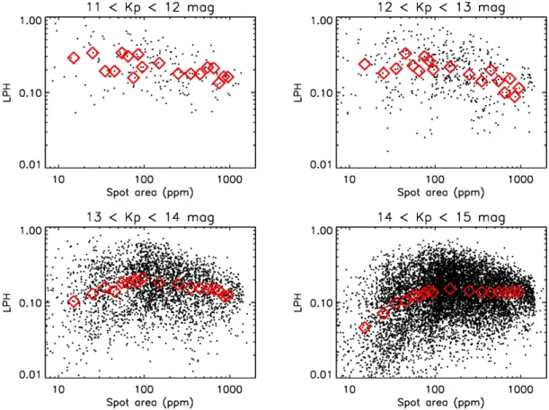
3.2. LPH dependence on spot area
The two examples in Sect.3.1illustrated how the period detection is affected by the activity level (Fig.1) and the amount of observational noise (Fig.2). Fig.3combines both of these effects by showing the LPH when the highest peak was found between 24–30 days, as a function of the sunspot coverage on the visible solar disc, averaged over the 4-year segment (in ppm), for different magnitudes. The red diamonds show
1The chosen segment slightly differs from the one chosen in the third panel Fig.1to demonstrate the effect of noise on the LPH.
Figure 2. Same as Fig.1but choosing the same light curve segment for three different noise realizations corresponding to 11th (left), 13th (middle), and 15th (right) Kepler magnitude. The LPH decreases towards fainter stars.
the median LPH values for the selected spot area bins to better illustrate the LPH dependence.
The upper left panel shows only stars brighter than 12th Kepler magnitude (i.e. with small noise levels). The LPH increases with decreasing spot area. As mentioned above, small spot coverages are typically found during activity minima when variabil-ity becomes faculae-dominated. Consequently, the light curves become more regular. A similar trend is found for stars between 12th and 13th magnitude but with larger scatter (upper right panel). Between 13th to 14th magnitude (lower left panel), the noise level becomes comparable to the variability amplitude during epochs of small spot coverages. As a result, the LPH drops for small coverages and the increase of the LPH with decreasing spot area can only be identified down to spot areas of 100 ppm. For the faintest stars down to 15th magnitude (lower right panel), the larger noise further decreases the LPH for small spot areas, and for spot areas above 100 ppm no trend can be identified any longer.
3.3. Period distribution
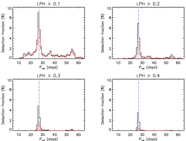
As shown in the previous section, the position of the highest peak and the associated LPH determine the period detection. The percentages of correct and false detections are given in Table 1. The period distribution is shown in Fig. 4 for different LPH
Figure 3. Local peak height (LPH) vs. spot area fraction for different Kepler magnitudes. The red diamonds show the median LPH values for the selected spot area bins. The very few peaks with LPH < 0.01 were excluded from the analysis.
constraints for the noise-free (black) and the noisy (red) case. From the upper left to the lower right panel, the LPH threshold increases from 0.1 to 0.4. Consequently, the detection fraction decreases, but also the number of false detections drops. The decrease of detections is even stronger for the noisy case. We note that also the false detections decrease more strongly for the noisy case (see Table 1). This is caused by the fact that a peak is more easily found in the noise-free case, but the associated period lies outside the range of 24–30 days, and is therefore counted as false detection. When measuring rotation periods in real data, the period is a priori unknown, and one has to assign a certain LPH threshold, for which periods are considered as significant. The upper left panel in Fig. 4 shows that even for small values (0.1 < LP H < 0.2), most detections are found at the correct (model) rotation period of 27 days. However, the number of false detections is also quite high (see Table 1). Further increasing the LPH threshold significantly decreases the number of false de-tections but also lowers the number of correct dede-tections. Finding an optimal LPH threshold that compromises between discarding correct detections and not having too many false periods is non-trivial. We stress that MMA14 required LP H > 0.3 to count the period as a real detection. As seen in the lower left panel, this
thresh-Figure 4. Rotation period distribution for different local peak heights of the noise-free (black) and noisy (red) cases. The blue dashed-dotted line indicates the model rotation period of 27 days.
LPH Detection False detection Noise-free Noisy Noise-free Noisy >0.1 23.8% 17.3% 35.2% 27.4%
>0.2 15.5% 7.4% 9.0% 4.5%
>0.3 9.5% 2.9% 1.9% 0.5%
>0.4 6.1% 1.0% 0.4% 0.0%
Table 1. Detections and false detections for different LPH for both the noise-free and noisy cases.
old eliminates almost all false detections but strongly decreases the number of real detections (see discussion below).
3.4. Detection rate
We now turn to the question how the period detectability is affected by stellar inclination and metallicity. For that purpose, we define the detection rate as the number of detections divided by the number of different Monte Carlo runs at a given parameter. In Fig. 5 we show the detection rate as a function of the inclination of the rotation axis of the model star (integrated over all metallicities) for different LPH values. The error bars indicate the square root of the number of detections divided
Figure 5. The detection rate as a function of inclination angle, integrated over all metal-licities, for different LPH thresholds. The error bars show the square root of the number of detections divided by the number of models at a given inclination.
by the number of models. As before, we consider the noise-free (left panel) and the noisy (right panel) cases separately.
The noise-free case qualitatively displays the same behavior for all LPH thresholds. As expected, the detection rate is zero for the pole-on view. However, when increas-ing the inclination angle the detection rate steeply increases to the maximum at an inclination near 20◦, and gradually decreases towards the equator-on view at 90◦. This result might be surprising at first glance but can be explained by the dominant contribution of faculae to brightness variability for stars with near-equatorial activity belts (similar to those on the Sun) observed close to the pole-on view (Shapiro et al. 2016). In such stars each facular feature spends roughly half a rotation period on the far-side of a star and the remaining half of the time near the limb on the visible disk. Faculae appear especially bright near the limb, and usually last for several stellar rotations. Consequently, the light curves of such stars appear more regular, leading to higher LPH values. We note that the calculations are performed assuming a solar latitudinal distribution of active regions. A change of the distribution would affect the visibility of the active regions, and consequently, the inclination angle corresponding to the maximum of the detection rate. However, we expect that a solar distribution is typical for stars with solar rotation period and temperature (see Sect.2.2).
In the noisy case (right panel) the detection rates are generally smaller (cf. Table1
and Fig. 4). While the curves have a similar shape to the noise-free cases, their maxima are shifted to higher inclinations. Such a shift is caused by the decrease of the amplitude of brightness variability with decreasing inclination (N`emec et al. 2020), and consequently a decrease of the signal-to-noise ratio. Consequently, the detection peak near 20◦ is suppressed, leaving a residual peak near 40◦. As already shown in Figs.3 and 4, the noise decreases the LPH such that only a few cases with LP H > 0.3 remain.
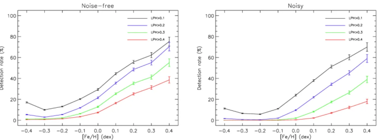
In Fig. 6 we show the detection rate as a function of metallicity (integrated over all inclinations) for different LPH values. We note that the qualitative shape of
Figure 6. The detection rate as a function of metallicity, integrated over all inclinations, for different LPH thresholds. The error bars show the square root of the number of detections divided by the number of models at a given metallicity.
the LP H > 0.1 curve is consistent with the one found in Witzke et al. (2020), who considered the noise-free case (see Sect. C in the appendix for the difference between the calculations in this study and those employed in Witzke et al. 2020). Fig. 6 shows that for both the noise-free (left panel) and the noisy (right panel) case, the detection rate increases with metallicity. This is caused by the stronger contribution of the faculae to the overall variability. Only for the cases LP H > 0.1 and LP H > 0.2, does the detection rate show a minimum at [Fe/H] = −0.3 dex or −0.2 dex (noisy), increasing again towards smaller metallicity values. We expect that this trend continues towards even smaller metallicities.
3.5. Comparison with observations
We now compare our detection rates (see Table 1) to period detections of solar-like stars in the MMA14 sample. As mentioned above, MMA14 used a relatively conservative detection threshold of LP H > 0.3. The bottom left panel of Fig. 4
and Table 1 indicate that this threshold represents only the tip of the iceberg: for LP H > 0.3 (noisy case), the rotation periods can be correctly detected for only 2.9% of our modeled light curves.
Galactic evolution models (van Saders et al. 2019) predict that 16% of the (dwarf) stars in the Kepler field with effective temperatures 5500 < Teff < 6000 K should
have rotation periods between 24–30 days (van Saders, private communications). Using the latest Kepler parameter catalog (Mathur et al. 2017), we select stars in this temperature range, with surface gravities log g > 4.2 to exclude more evolved stars, and brighter than 15th Kepler magnitude (following the selection criteria used in Reinhold et al. 2020). We further restrict the catalog metallicities to −0.45 < [Fe/H] < 0.45 dex, which corresponds to the range of simulated metallicities (see Fig. A.1). Selecting such stars from tables 1 and 2 in MMA14 yields N = 16890 stars. Among those, only 16% will have periods between 24–30 days, and according
to our analysis, only 2.9% of these stars will have detectable periods. Thus, we estimate that Ndet = N ∗ 0.16 ∗ 0.029 = 78 stars should have detectable periods.
MMA14 found 455 stars in this parameter range with periods 24 ≤ Prot ≤ 30 days.
However, the vast majority of these stars exhibits variability levels much higher than the Sun, and represent a regime of variability very different from that of the Sun (Reinhold et al. 2020; Zhang et al. 2020; Is,ık et al. 2020). Consequently, the light
curves of these stars cannot be accounted for by our model. To correct for such stars, we followed the approach ofWitzke et al.(2020) and selected the stars with variability (regressed to solar values of effective temperature, metallicity, and rotation period, see Fig. S8 and its detailed discussion in Reinhold et al. 2020) below 0.18%, which corresponds to the maximum variability of the Sun over the last 140 years. All in all, only 73 out of the 455 stars satisfied such a criterion. This number is gratifyingly close to our estimate of 78 stars.
4. CONCLUSIONS
In this study we identified biases in the period determination of stars with solar-like variability. The detection rates among these stars are lower than for stars of other spectral types. In particular, only 2.9% of them would be detectable using the thresholds set in MMA14. This is mainly caused by the small variability amplitudes of the rotational tracers and their relatively short lifetimes compared to the rotation period.
The very low detection rate explains the large discrepancy between the number of measured rotation periods (MMA14), and those predicted by Galactic evolution models (van Saders et al. 2019). The predicted number of stars with detectable periods (78), and that for which rotation periods have actually been measured (73), is remarkably similar. Fig. 4 shows that many more rotation periods of solar-like stars may be measured when lowering the thresholds in the automated period surveys. However, this will also add a number of false periods, depending on how the thresholds are set.
Our study revealed that the rotation periods of most solar-like stars will go unde-tected using standard frequency analysis tools. Thus, we emphasize the importance of alternative methods for period detection such as the GPS method (Shapiro et al. 2020;
Amazo-G´omez et al. 2020) or new approaches based on Gaussian process regression (Foreman-Mackey et al. 2017; Angus et al. 2018; Kosiarek & Crossfield 2020).
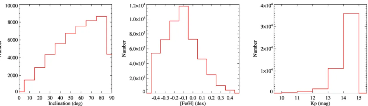
Figure A.1. Input distributions of inclination angles (left) and metallicities (middle), and Kepler magnitudes (right) of the Monte Carlo simulation.
ACKNOWLEDGMENTS
We would like to thank Jennifer van Saders for providing model numbers and for helpful discussion. This work has received funding from the European Research Coun-cil (ERC) under the European Union’s Horizon 2020 research and innovation pro-gramme (grant agreement No. 715947). This work has been partially supported by the BK21 plus programme through the National Research Foundation (NRF) funded by the Ministry of Education of Korea. We would like to thank the International Space Science Institute, Bern, for their support of science team 446 and the resulting helpful discussions.
APPENDIX
A. MONTE CARLO INPUT DISTRIBUTION
Fig. A.1shows the distributions of input parameters used in the Monte Carlo sim-ulation. The first panel shows the distribution of inclination angles. It can be shown that isotropic inclination angles i exhibit a uniform distribution in cos i (see e.g.
http://keatonb.github.io/archivers/uniforminclinationfor a detailed derivation). The last bin of the distribution (85 − 90◦) only contains half the number of realizations because no inclination angles greater than 90◦ exist. The same argument applies to the first bin from 0 − 5◦.
The middle panel shows the distribution of metallicities of the solar-like stars in the Kepler field. The catalog values were adapted from Mathur et al.(2017) and the selection of solar-like stars can be found in Reinhold et al.(2020). We note that the Sun ([Fe/H] = 0) is slightly more metal-rich than the peak of the distribution.
The last panel shows the apparent magnitudes of the stars in the Kepler field. It is obvious that the majority of stars is very faint. Since the stellar magnitudes define the noise in the light curves, it is crucial to adapt this distribution for the noise model (seeReinhold et al. 2020) to make realistic predictions about stars in the Kepler field.
B. GENERATING LIGHT CURVES
The total spectral flux at a certain time is composed of fluxes emerging from surface areas with different levels of magnetic activity. Following the detailed description in
Shapiro et al.(2014), we decompose the spectral flux from a star, F , into contributions from the quiet stellar region (FQ), faculae (Ffac), and spots (Fspot):
F (λ) = FQ(λ) + Ffac(λ) + Fspot(λ), (B1)
where λ is the wavelength. For the quiet stellar region, the disc-integrated flux FQ(λ)
is obtained by integrating
FQ(λ) =
Z 1
0
IQ(λ, µ)ω(µ)dµ, (B2)
where ω(µ) = 2πµ(rstar/dstar)2 is a weighting function with the stellar radius, rstar,
and the distance between the star and the observer, dstar. The emergent intensity,
IQ(λ, µ), also depends on µ, which is the cosine of the angle between the observer’s
direction and the local stellar radius. In this formulation the stellar disc center is associated with µ = 1 and the limb with µ = 0.
Both faculae and spots are taken into account through their contrast with respect to the quiet regions. Therefore, the contribution of faculae is defined as
FF ac(λ) =
Z 1
0
αF ac(µ) [IF ac(λ, µ) − IQ(λ, µ)] ω(µ)dµ, (B3)
where the fractional coverage of the ring corresponding to a given µ by faculae is given by the function αF ac(µ).
The contribution from spots consists of those from spot umbrae and spot penum-brae: Fspot(λ) = Z 1 0 αpen(µ) (Ipen(λ, µ) − IQ(λ, µ)) ω(µ)dµ + Z 1 0 αumb(µ) (Iumb(λ, µ) − IQ(λ, µ)) ω(µ)dµ, (B4)
where Iumb and Ipen are the emergent intensities from the spot umbrae and spot
penumbrae, respectively, and the αumb and αpen denote the corresponding surface
coverages.
The surface coverages for the magnetic features (i.e. αFac, αumb and αpen) used
in this work are taking from N`emec et al. (2020). Furthermore, calculations of the emergent intensities for all stellar regions follow the approach used in Witzke et al.
(2020), but with a small modification which is explained in Appendix C.
C. CALCULATING EMERGENT INTENSITIES
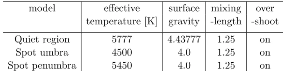
The model atmospheres and corresponding emergent spectra computed by Unruh et al.(1999) for the solar faculae, spots, and quiet regions (hereafter, original models)
model effective surface mixing over temperature [K] gravity -length -shoot
Quiet region 5777 4.43777 1.25 on
Spot umbra 4500 4.0 1.25 on
Spot penumbra 5450 4.0 1.25 on
Table 2. Input parameters for model atmospheres in radiative equilibrium.
proved to be very successful in reproducing the solar brightness variations with high accuracy (Krivova et al. 2003; Solanki et al. 2013;Ermolli et al. 2013).
Here, we extend the intensities for different surface components to different metal-licities following the approach outlined in Witzke et al. (2018,2020), but with slight modifications to cover a broader metallicity range. In our modeling approach, we aim to match the intensity contrasts for the solar metallicity as closely as possible to the original models. Thus, in the first step we searched for the model parameters (input parameters for calculating stellar atmospheres with ATLAS9), such as con-vection settings, surface gravity and continuum opacity sources for the quiet Sun, spot-umbra and spot-penumbra, to match the original models and spectra by Unruh et al.(1999). The closest match is achieved by the parameters listed in Table2. Then for the generation of the faculae model we assumed that the temperature difference, ∆T, and pressure difference, ∆P , as a function of column mass between the original facular and quiet Sun models are the same as between our new facular and quiet Sun models.
Finally, to calculate atmospheric models for different metallicity values, we first generated atmosphere models for the quiet regions and the spots assuming radiative equilibrium. Then we followed up on the Witzke et al.(2018) approach and assumed that a change of the metallicity value has the same effect on the temperature and pressure structures of the quiet Sun and faculae. Using the quiet stellar atmosphere models for different metallicities, we applied the solar ∆T and ∆P with column mass to calculate the facular models. Using these atmospheric models for the quiet regions and magnetic features, we generated the emergent intensities Iλ,µ for each metallicity
value using the MPS-ATLAS code (Witzke et al. in prep.).
REFERENCES
Aigrain, S., Llama, J., Ceillier, T., et al. 2015, MNRAS, 450, 3211,
doi: 10.1093/mnras/stv853
Amazo-G´omez, E. M., Shapiro, A. I., Solanki, S. K., et al. 2020, A&A, 636, A69, doi: 10.1051/0004-6361/201936925
Angus, R., Morton, T., Aigrain, S., Foreman-Mackey, D., & Rajpaul, V. 2018, MNRAS, 474, 2094,
doi: 10.1093/mnras/stx2109
Cameron, R. H., Jiang, J., Schmitt, D., & Sch¨ussler, M. 2010, ApJ, 719, 264, doi: 10.1088/0004-637X/719/1/264
Ermolli, I., Matthes, K., Dudok de Wit, T., et al. 2013, Atmosph. Chem. Phys., 13, 3945, doi:10.5194/acp-13-3945-2013 Foreman-Mackey, D., Agol, E.,
Ambikasaran, S., & Angus, R. 2017, AJ, 154, 220,
doi: 10.3847/1538-3881/aa9332
He, H., Wang, H., & Yun, D. 2015, ApJS, 221, 18,
doi: 10.1088/0067-0049/221/1/18 Is,ık, E., Shapiro, A. I., Solanki, S. K., &
Krivova, N. A. 2020, ApJL, 901, L12, doi: 10.3847/2041-8213/abb409
Jiang, J., Cameron, R. H., Schmitt, D., & Sch¨ussler, M. 2011, A&A, 528, A82, doi: 10.1051/0004-6361/201016167 Karoff, C., Metcalfe, T. S., Santos, ˆA.
R. G., et al. 2018, ApJ, 852, 46, doi: 10.3847/1538-4357/aaa026 Kosiarek, M. R., & Crossfield, I. J. M.
2020, AJ, 159, 271,
doi: 10.3847/1538-3881/ab8d3a
Krivova, N. A., Solanki, S. K., Fligge, M., & Unruh, Y. C. 2003, A&A, 399, L1, doi: 10.1051/0004-6361:20030029 Lanza, A. F., & Shkolnik, E. L. 2014,
MNRAS, 443, 1451,
doi: 10.1093/mnras/stu1206
Mathur, S., Huber, D., Batalha, N. M., et al. 2017, Astrophys. J., Suppl. Ser., 229, 30,
doi: 10.3847/1538-4365/229/2/30 McQuillan, A., Mazeh, T., & Aigrain, S.
2014, Astrophys. J., Suppl. Ser., 211, 24, doi: 10.1088/0067-0049/211/2/24 N`emec, N. E., Shapiro, A. I., Krivova,
N. A., et al. 2020, A&A, 636, A43, doi: 10.1051/0004-6361/202037588 Reinhold, T., Shapiro, A. I., Solanki, S. K., et al. 2020, Science, 368, 518. https://arxiv.org/abs/2005.01401 Schuessler, M., & Solanki, S. K. 1992,
A&A, 264, L13
Shapiro, A. I., Amazo-G´omez, E. M., Krivova, N. A., & Solanki, S. K. 2020, A&A, 633, A32,
doi: 10.1051/0004-6361/201936018
Shapiro, A. I., Solanki, S. K., Krivova, N. A., et al. 2017, Nature Astronomy, 1, 612, doi:10.1038/s41550-017-0217-y —. 2014, A&A, 569, A38,
doi: 10.1051/0004-6361/201323086 Shapiro, A. I., Solanki, S. K., Krivova,
N. A., Yeo, K. L., & Schmutz, W. K. 2016, A&A, 589, A46,
doi: 10.1051/0004-6361/201527527 Solanki, S. K. 2003, A&A Rv, 11, 153,
doi: 10.1007/s00159-003-0018-4 Solanki, S. K., Krivova, N. A., & Haigh,
J. D. 2013, Ann. Rev. Astron. Astrophys., 51, 311, doi:10.1146/ annurev-astro-082812-141007
Solanki, S. K., Usoskin, I. G., Kromer, B., Sch¨ussler, M., & Beer, J. 2004, Nature, 431, 1084, doi:10.1038/nature02995 Unruh, Y. C., Solanki, S. K., & Fligge, M.
1999, A&A, 345, 635
Usoskin, I. G., Solanki, S. K., &
Kovaltsov, G. A. 2007, A&A, 471, 301, doi: 10.1051/0004-6361:20077704 van Saders, J. L., & Pinsonneault, M. H.
2012, ApJ, 746, 16,
doi: 10.1088/0004-637X/746/1/16 van Saders, J. L., Pinsonneault, M. H., &
Barbieri, M. 2019, ApJ, 872, 128, doi: 10.3847/1538-4357/aafafe
Witzke, V., Reinhold, T., Shapiro, A. I., Krivova, N. A., & Solanki, S. K. 2020, A&A, 634, L9,
doi: 10.1051/0004-6361/201936608 Witzke, V., Shapiro, A. I., Cernetic, M.,
et al. in prep., A&A
Witzke, V., Shapiro, A. I., Solanki, S. K., Krivova, N. A., & Schmutz, W. 2018, A&A, 619, A146,
doi: 10.1051/0004-6361/201833936 Zhang, J., Shapiro, A. I., Bi, S., et al.
2020, ApJL, 894, L11,
![Figure 1. Top row: Model light curve (black) with an inclination of i = 40 ◦ and solar metallicity [Fe/H] = 0, with three randomly chosen 4-year segments (green)](https://thumb-eu.123doks.com/thumbv2/9libnet/5470271.105852/6.918.141.775.93.569/figure-model-black-inclination-metallicity-randomly-chosen-segments.webp)