Motion planning of a mechanical snake using neural networks

í á 'S t l i i

pl ШШІЩШ Ш

іі

MOTION PLANNING OF A MECHANICAL SNAKE

USING NEURAL NETWORKS

A THESIS

SUBMITTED TO THE DEPARTMENT OF ELECTRICAL AND ELECTRONICS ENGINEERING

AND THE INSTITUTE OF ENGINEERING AND SCIENCES OF BILKENT UNIVERSITY

IN PARTIAL FULFILLMENT OF THE REQUIREMENTS FOR THE DEGREE OF

MASTER OF SCIENCE

By

Barış Fidan July 1998

I certify that I have read this thesis and that in my opinion it is fully adequate, in scope and in quality, as a thesis for the degree of Master of Science.

Prof. Dr. M. Erol Sezer(Sui3ervisor)

I certify that I have read this thesis and that in my opinion it is fully adequate, in scope and in quality, as a thesis for the degree of Master of Science.

Prof. Dr. A. Bülent Özgüler

I certify that I have read this thesis and that in my opinion it is fully adeqiuite, in scope and in quality, as a thesis for the degree of Master of Science.

Assoc.vProf. Dr. Billur Barshan

Approved for the Institute of Engineering and Sciences: (

Prof. Dr. Mehmet Baray \f.

ABSTRACT

M O T IO N P L A N N IN G O F A M E C H A N IC A L S N A K E USING N E U R A L N E T W O R K S

Barış Fidan

M .S. in Electrical and Electronics Engineering Supervisor: Prof. Dr. M . Erol Sezer

July 1998

In this thesis, an optimal strategy is developed to get a mechanical snake (a robot composed of a sequence of articulated lirdcs), which is located arbitrar­ ily in an enclosed region, out of the region through a specified exit without violating certain constraints. This task is done in two stages: Finding an op­ timal path that can be tracked, and tracking the optimal path found. Ecich stage is implemented by a neural network. Neural network of the second stage is constructed by direct evaluation of the weights after designing an efficient structure. Two independent neural networks are designed to implement the first stage, one trained to implement an algorithm we have derived to gen­ erate minimal paths and the other ti'ciined using multi-stage neural network approach. For the second design, the intuitive multi-stage neurcil network back propagation approach in the literature is formalized.

Keywords : Mechanical snake, articulated robot arm, motion planning, path

planning, minimal path, back propagation, neural network, multi-stage neural network.

ÖZET

m e k a n i k b i r Y IL A N IN D E V İN İM İN İN Y A P A Y SINIR A Ğ L A R I İLE T A S A R L A N M A S I

Barış Fidan

Elektrik ve Elektronik Mühendisliği Bölümü Yüksek Lisans Tez Yöneticisi: Prof. Dr. M . Erol Sezer

Temmuz 1998

Bu tezde, kapalı bir alanın içine gelişigüzel yerleştirilen bir mekanik yılanın (eklemlerle birleştirilmiş bir dizi milden oluşan robot), bazı sınırlamaları boz­ madan, bu alanın belirlenmiş bir çıkışından dışarı çıkarılmasını sağlayacak bir eniyi yöntem geliştirilmiştir. Bu yöntem iki evreden oluşmaktcidır; izlenebilecek eniyi yolun bulunması ve bulununan eniyi yolun izlenmesi. Bu evrelerin her biri bir yapay sinir ağı tarafından yürütülmektedir, ikinci evreyi yürüten yapay sinir ağı etkili bir yapının tasarlanmasından sonra, bu yapı içindeki ağırlıkların değerlerinin doğrudan bulunması ile oluşturulmuştur. Birinci evreyi yürütmek için birbirinden bağımsız iki yapay sinir ağı tasar­ lanmıştır. Bunların ilki en kısa yolları üretmek için geliştirdiğimiz bir algorit­ mayı yerine getirmek üzere eğitilmiştir. İkincinin eğitiminde i.se çok evreli sinir ağları yaklaşımı kullanılmıştır, ikinci tasarı için, literatürde sezgisel olarak yer alan çok evreli sinir ağlarında geriyayılım yaklaşımı netleştirilmiştir.

Anahtar Kelimeler : Mekanik yılan, eklemli robot kolu, devinim tasarımı, yol

ACKNOWLEDGEMENT

I would like to express my deep gratitude to my supervisor Prof. Dr. Mesut Erol Sezer for his guidance, suggestions and invaluable encouragement through­ out the development of this thesis.

I would like to thaidi to Prof. Dr. Arif Bülent Özgüler and Assoc. Prof. Dr. Billur Barshan for reading and commenting on the thesis aird for the honor they gave me by presiding the jury.

I would like to thank to my family especially for their moral support.

Sincere thanks are also extended to everybody who has helped in the develop­ ment of this thesis in some way.

to my parents,

and my brother

TABLE OF CONTENTS

1 IN TR O D U CTIO N 1

2 NEURAL N E TW O R K S IN ROBOTICS AN D CONTROL 4

2.1 Multilayer Neural Networks 4

2.2 Training and Back P r o p a g a tio n ... 5

2.3 Applications of Neural Networks in Robotics and Control . . . . 8

2.4 Multi-stage Neural N etworks... 8

3 M O TIO N PLAN N IN G OF A M ECH AN ICAL SNAKE 12

3.1 Introdu ction... 12

3.2 Definition of the Problem 14

3.3 Generation of P a t h ... 17

3.4 Structure of the Complete C o n tr o lle r ... 20

3.5 Ti'cicking the Generated Path 22

4 M IN IM A L PATH APPROACH 34 4.1 Minimal Paths on the Right Half P la n e ... 34

4.2 Design of the Path Generator Neural N e tw o r k ... 46

4.3 R esu lts... 48

5 MULTI-STAGE NEURAL N E T W O R K APPROACH 54

5.1 Multi-Stage Neural Networks with Identical Stages 54

5.2 Application to the Pcith Generation P ro b le m ... 60

5.3 R esu lts... 63

6 CONCLUSION 67

APPENDICES 68

A Back Propagation with Momentum 69

A .l 2-Layer Neural N etw orks... 69

A . 2 3-Layer Neural N etw orks... 71

B Proofs of the Facts on Tracking the Generated Path 73

B . l Proof of Fact 3.1 73

B.2 Proof of Fact 3.2 74

C Determination of K ^ a x "^8

LIST OF FIGURES

2.1 An ?7-inpiit neuron... 5

2.2 Multilayer neurcil networks used in the thesis. 6 2.3 A finite-dimensional discrete-time system with a controller. . . . 9

2.4 A"-stage neural network representation of a A'-step process. . . . 10

3.1 Simplified structure of the mechanical snake... 15

3.2 Basic linear motion pattern... 16

3.3 Problem 3.1... 17

3.4 (a) Piece-type definitions, (b) The initial configuration repre­ sented by {x ,y , 180°, —1, —1,1, —1,0,1,1). 18 3.5 Path generator neural network. 19 3.6 Complete neural network controller scheme for the adjusted ini­ tial configuration... 21

3.7 NNtrack... 25

3.8 (a) NNupdate- (b) NNccnv... 26

3.10 (a) NN^. (b) NNc. (c) NN^,1. (d) NN^2- 28

3.11 (a) NNe. (b) NN^od... 29

3.12 A sample adjustment proce,ss... 31

3.13 (a) The scheme for the adjustment of the initial configuration.

(b) NN^dji. 32

3.14 NNadj2. 33

4.1 Minimal path candidates for IP = (;r, y) and (¡)q = 6... 38

4.2 Algorithm 4.1: (a) location of L C {x ,y ,0 ) and R C {x ,y ,9 ) and (b) sample minimal path for the first case in Step 3(a).ii... 42

4.3 Algorithm 4.1: Sample minimal paths for (a) the second case in Step 3(a).ii, (b) Step 3(b), (c) the first case in Step 4(a).ii, (d) the second case in Step 4(a).ii, (e) Step 4(b) and (f) StejD 5. 43

4.4 Outputs of the (7''"'‘ -code of Algorithm 4.1 for the examples illustrated in Figures 4.2(b), 4.3(a) and 4.3(b)... 44

4..'5 Outputs of the C'‘'"''-code of Algorithm 4.1 for the examples illustrated in Figures 4.3(c), 4.3(d), 4.3(e) and 4.3(f)... 45

4.6 Construction of NNpath using NNrj blocks... 47

4.7 Blocks A N Dq and OB-a, and the 3-state hardlirniter used in

A N Dg. 47

4.8 Desired outputs for {x ,y ) € Ri (defined in Problem 3.1) for

^ _ 0 JL 2^ . . . . 49

V u, ···> 12...

4.10 (a) Minimal paths and (b) the desired outputs obtciined using the original forms of i?_i, Ro and Ri for the initial triples (i) a; = 12, y = 5, ^ = 30°, (ii) x = 5, ?y = 0, d = 0°, (iii)

X = 5, y — 0, 0 = 180°, (iv) X = 1, y — 1,

6

X = 4, y = - 2 , 0 = 90°... 51

4.11 Outputs for the neural network weights of epoches (a) 100, (b) 1000 and (c) 9000 for the initial triples (i) x = 12, y = 5, 0 = 30°, (ii) .-r = 5, y = 0, 0 = 0°, (iii) a; = 5, y = 0, 0 = 180°, (iv) = 1, 2/ = 1, 0 = .30°, (v) x = 4, y = - 2 , 0 = 90°... 52

4.12 Sample process using the complete neural network controller. . . 53

5.1 A finite-dimensional discrete-time system with a controller. . . . 55

5.2 /-f-stage neural network repre.sentation of a A'-step process. . . . 56

5.3 D{.) for the path generation problem... 62

5.4 Average error during the training process. 64 5.5 Outputs for the neural network weights of epoches (a) 100, (b) 1000 and (c) 5000 for the initial triples (i) x = 12, y = 5, 0 = 30°, (ii) .T = 5, y = 0, 0 = 0°, (iii) .T = .5, y = 0, 0 = 180°, (iv) X =

1^ rj = 1, 0 =

B .l Fact 3.1... 74

B. 2 Fact 3.2... 75

C . l Ji, Ji+i, Ji+2, Ji+3 on a circular arc of radius ... 79

LIST OF TABLES

3.1 Segment solenoids and joint angles during a linear motion cycle. 15

3.2 Joint angles during a general motion cycle... 24

3.3 Joint angle increments during a general motion cycle... 25

3.4 Possible input-output pairs for NN

^2

Chapter 1

INTRODUCTION

In robotics, the uttermost aim is to construct a physical device to simulate aspects of human behavior involving interaction with the world, such as ma­ nipulation or locomotion. To make a robot useful, an efficient conti'ol unit is required to control the robot’s motions and the forces to be applied to the environment. Since the aim is to simulate human behavior, it seems feasible to construct emulators of the control units of humans as efficient robotic control units.

This idea directed the researchers towards the neural structures in living or­ ganisms and motivated them to study construction of artificial neural networks, networks with structures similar to those in humans containing processor units which mimic biological neurons. Usage of artificial neural networks in robotics and control has been popular for four decades. Because of their ability to solve highly nonlinear problems, neural networks have been used not only in robotics and control but also in many other areas such as optimization, signal process­ ing, computer .systems, statistical physics and communication [1, 2, 3, 4, .5].

Design of a useful neural network can be realized in two stages; choosing a suitable network structure and adjustment of the parameters, called weights, in this structure. In general, the weights can not be selected directly to fulfill an arbitrary task. In such a case, weights are adjusted by means of a training

process. In the training process, the neural network is stimulated by the envi­ ronment and the weights of the network are updated according to the result of the stimulation repetitively till the desired performance is obtained.

Most of the training techniques in the literature are gradient descent based. The basic technique used in this thesis is also a popular gradient descent based technique, Back Propagation. In basic Back Propagation algorithm, a set of input-desired output pairs is needed to train the neural network. However, for many tasks, such a set is not available. Such ci case is the problem of driving a discrete-time plant from an initial state Zq to a desired state Zd in an unknown number of steps.

In this general |)roblem, the only information in hand to train the controller is the desired outputs for the hist steps. Desired outputs for the intermediate steps and number of steps to reach the desired final state are not available for any of the initial states in the training set. Using a multi-stage structure is beneficial in this case.

A multi-stage neural network is an integrated neural network composed of a number of cascaded neural networks. In [6] and [7], Nguyen and Widrow use a /i-stage neural network to represent a A^-step process to solve the problem above and train a controller which backs a trailer truck to a loading dock using this approach. However, the equivalent errors in the method are not well- defined and explicit formulation of the back propagation through A'-stages is not given. In this work, we will introduce a similar approach to apply Back Propagation in multi-stage neural networks with identical stages and formulate the approach.

The neural networks designed in this work are used for motion planning of a mechanical snake, a robot with a structure and a motion pattern similar to those of a snake. A mechanical snake will be useful in situations where it is necesaary to crawl into places which are too dangerous or too narrow for people to enter, such as disaster areas and nuclear power plants with narrow vessels.

Efficiency of the motion for a mechanical snake is important, as it is for any mobile robot in general. Generating collision-free motion of satisfactory

quality is one of the main areas of interest in robotics [8]. For the case of the mechanical snake, our aim is to generate smooth minimal paths, which can be tracked unobtrusively, to exit an enclosed area, and to track the generated paths efficiently.

The thesis is organized as follows: Basics of neural networks and applica­ tions of neural networks in robotics and control are reviewed and multistage neural networks are introduced in Chapter 2.

In Chapter 3, structure of the mechanical snake is determined, and the problem of exiting from the enclosed area is defined. Later, a structure for the complete controller is determined and the neural network for the path tracking task is designed directly.

In Chapter 4, an algorithm to generate minimal paths with maximum cur- vatui’es in the right half plane is derived, and this algorithm is converted to a neural network controller which generates minimal paths.

In Chapter 5, our approach to apply Back Propagation in multi-stage neural networks with identical stages is introduced, and this approach is used to solve the path generation problem.

Chapter 2

NEURAL NETWORKS IN

ROBOTICS AND CONTROL

2.1

Multilayer Neural Networks

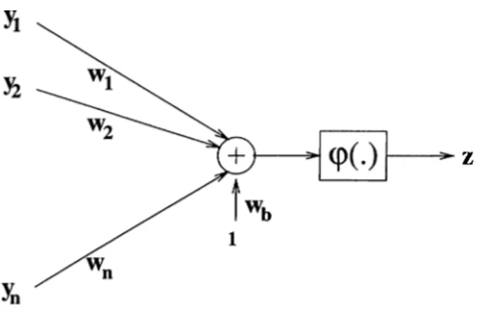
In many areas of research, cin artificial neural network refers to a structure designed to implement or approxinicite an arbiti'ciry function o = 6 '(x), mim­ icking the neural structures in living creatures. This structure is composed of basic multi-input-single-output units called neurons. In the most general model for an ??.-input neuron, weighted summation of n inputs is biased and passed through an activation function <p(.). The output for the neuron in Figure 2.1 is given by:

= (p (^

+

i=l

(

2

1

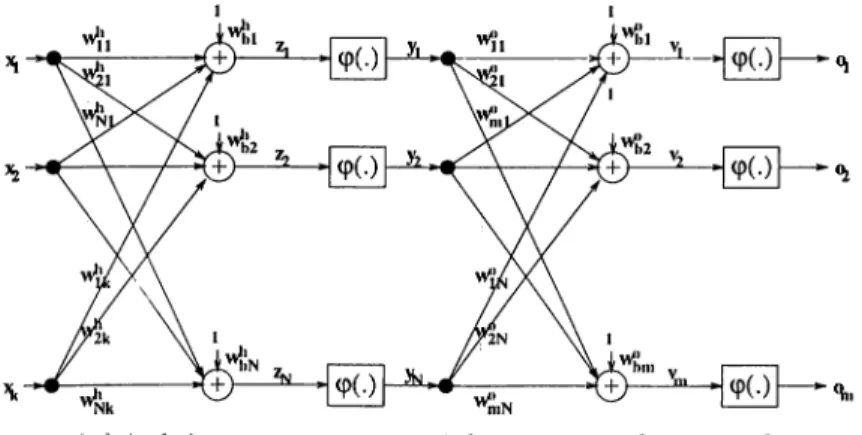
A multilayer neurcil network is a regular network in which the neurons are collected in a number of layers and the connections are settled between these layers. The layer which is closest to the output and which has outputs as

Figure 2.1: An ?r-input neuron.

the outputs of the neural network is called the output layer. Other hiyers are called hidden layers. The multilayer neural networks used in this thesis are 2- layer and 3-layer neural networks. A:-input-?7i-output 2-layer and 3-lciyer neural networks are pictured in Figure 2.2.

2.2

Training and Back Propagation

Design of a useful neural network can be realized in two stages. In the first stage, a suitable network structure is chosen, and in the second, the weights in the structure are adjusted so that the outputs are close enough to the desired values.

In general, direct selection of the weights to fulfil an arbitrary task is not feasible. In such cases, random initial values are assigned to the weights, and adjustment of the weights is done by means of a process of stimulation by the environment in which the neural network is embedded, which is Ccilled training.

Training processes can be divided into two groups as supervised training and unsupervised training. In supervised training, weights are adjusted according to the error measured as the distance between the actual output o and the desired output d. In unsupervised training, the desired outputs are not known, and learning must be accomplished based on observations of responses to inputs about which we have marginal or no knowledge [9, page 57]. In this thesis, we

(a)A A:-input-?7г-output 2-layer neural network

(b)A A;-input-?n-output 3-layer neural network

have used supervised training processes. The distance used in these processes is the Euclidean distance, and the error i'unction E lor a desired output - ¿ictual output pair d - o is defined as:

E \ l|d-o|

(2.2)

One of the mostly used supervised training techniques is Back Propagation.

Back Propagation is a gradient descent based algorithm, in which the weights are changed in the opposite direction of the gradient of the error function in the weight space. In the basic Back Propagation, the update for an arbitrary weight w in the neural network at step n of training process is given by

Aw{n) = —7]dE{n)

dio (2..3)

where 77 is a positive constant to be determined by the designer called the learn­

ing constant. In the thesis, we have used Back Propagation with Momentum,

in which the update in the previous step is used to speed up the convergence of the weights;

. . ^ dE{n)

Atu{n) = —7]——---- 1- aAw[n — 1)

ow (2.4)

where 0 < a < 1 is the momentum constant to be determined. The explicit equations of Back Propagation with Momentum for the neural networks in Figure 2.2 are given in Appendix A.

In a training process using Back Propagation, firstly, a training set of inputs is determined and desired outputs for these outputs are computed. Secondly, initial weights of the neural network and parameters of the Back Propagation Algorithm are set. Initial weights are generally selected as random numbers. Then, Back Propagation is applied for each element in the training set. One run is called an epoch. After each epoch, the average error for the set is computed. The algorithm is run for a sufficient number of epoches, till the average error falls below a predefined value e.

2.3

Applications of Neural Networks in Robotics

and Control

In robotics and control problems, the final ciirn is generally to implement a highly nonlinear task using linear devices and devices with nonlinearities of certain types. Since dealing with such highly nonlinear problems directly is too difficult and time consuming, different techniques of approximation are deyeloped to simplify these problems.

Until the last four decades, the usual attempt to such a nonlinear problem had been to determine some critical operating points, to linearize the equations of the problem around these points and to use the known linecir system tech­ niques. Since this attempt may not always be feasible or may be too costly, different approaches are needed.

Based on this need, researchers tried to adapt the perfect control structures and learning strategies of animals and humans to highly nonlinear systems, and usage of neural networks in control and robotics became populai· in recent decades[2, 5, 10, 11, 12, 13].

In the literature of the last three decades, many examples of applications of neural networks in function approximation, optimization, system identification, adaptive control, associative memory design, pattern classification, pattern recognition, sensor-based robotics, kinematic control of robots, path planning, .sensing-motion coordination can be seen[2, 4, .5, 10, 11, 13, 14, 15, 16, 17].

2.4

Multi-stage Neural Networks

A multi-stage neural network is a large neural network composed of a number

of cascaded neural networks. Such a structure is useful if the task of the neural network to be designed can be partitioned into separate simpler subtasks. In such a case, complementary neural networks are designed for these subtasks and are combined as a single network [18, 19].

The multi-stage structure is also beneficial for control problems in which the controller has to drive the plant lor a number steps to achieve the task, and only the desired output for the final step is available. In [6] and [7], Nguyen and Widrow show how the multi-stage structure can be used for controlling nonlinear dynamic systems, and apply this approach to the Truck Backer-

Upper Problem.

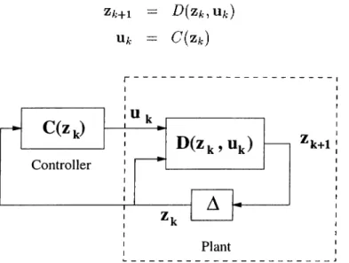
A finite-dimensional discrete-time controller can be represented as in Fig­ ure 2.3. Here Za, and Zk+i denote the current and next states of the plant respectively, and Ufc is the control signal given to the plant by the controller. Plant and controller equations for this scheme are as follows:

Za,+1 = Z?(Zfc,UA;)

UA: = C{Zk)

(2.5) (2.6)

'k+1

Figure 2.3: A finite-dimensional discrete-time system with a controller.

A common problem for such a scheme is to drive the plant from an initial state Zo to a desired state Zd in an unknown number of steps. In the Truck Backer-Upper example, the aim is to design a controller to back a trailer truck to a loading dock by only backing (i.e., going forward is not allowed) starting at an arbitrary initial position. The speed of the truck is assumed to be constant, and only the instantaneous steering angles of the truck determine the backing- path. If we discretize the problem, that is if the truck is moved for a number of constant-angle steps, the discrete-time controller is required to give a sequence of steering signals during the process. For this problem, Za· and z^+i denote the

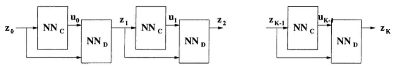
Figure 2.4: A'-stage neural network representation of a A'-step process.

position and the head direction of the truck-trailer in the current and the next step, Uk is the steering signal given by the controller, and Zj is the position vector of the parking dock augmented with a possible direction parameter denoting that the rear of the trailer is parallel to the dock.

In the multi-stage approach to design a neural network controller for this problem, the plant block can be approximated by an emulator neural network

N No, and if we denote the neural network controller by N No, a A^-step process

can be represented by a A"-stage neural network composed of K cascaded identical N N c-N N o pairs as in Figure 2.4.

Here, the actual ciim is to adjust the weights of the controller neural net­ work. The plant-emulator neural network is designed only to have a structure and an expression for the plant which can be easily used for training the con­ troller. Instead of a neural network, any smooth function D{.) emulating the plant can be used. A method to design an emulator neural network is given in [

6

For an initial point Zq in the training set, the system is run till a stopping event occurs. Assuming that the number of steps of the process is K, the final error E = \ ||zd —Za'II^ (z^ is the pre-determined desired output for Zq) can be back propagated through the plant emulator to find an equivalent error for the controller in the A^th stage. This equivalent error can be used to apply Back Propagation to the controller neural network in the A^th stage. The equivalent error can be back-propagated through all stages similarly to apply the Back Propagation Algorithm in all K stages, and weight updates for each stage can be determined. Weight update for one run can be found as the sum of the individual weight updates for the K stages.

error in the method is not well-defined and there is no explicit formulation of the back-propagation through K-stages. In Chapter 5, we will describe and formulate a slightly different approach to aj^ply Back Propagation in multi­ stage neural networks with identical stctges.

Chapter 3

MOTION PLANNING OF A

MECHANICAL SNAKE

3.1

Introduction

In robotic designs, designers are generally inspired by an animal that hiis the characteristics which are required to exist on the device to be designed. Snake, with its quick and calm motion ability in cluttered or tight areas, is such an animal. We will call a robot with a structure and a motion pattern similar to those of a snake a mechanical snake.

Such a robot will be useful when it is necessary to crawl into places which are too dangerous or too narrow for people to enter. Nuclear power plants with narrow vessels, disaster areas, military surveillance tasks are examples for these situations [20].

The bcisic design of a mechanical snake can be done in two steps, design of its structure and design of its motion pattern. There are various studies on the design of flexible-articulated structures. These structures are designed either to obtain a more efficient robot arm [21] or to realize the idea of producing

snake-like mobile robots [22, 20].

Motion jDatterns of biological snakes can be divided into four groups as

lateral undulation, rectilinear locomotion, sidewinding, cind concertina motion.

In lateral undulation, the snake undulates laterally b}^ bending the forward part of its body to establish a wavelike muscular contraction traveling down the snake’s trunk. The wavelike contractions cause the snake’s body to exert lateral forces on irregularities on the path, such as small elevations and depressions, pebbles, etc. The snake in effect pushes itself off from such points to go forward. During the motion, the snake sets its body in patterns of loops according to the irregularities, with the outside of each loop forming a contact point, and these patterns constitute the S-shaped path to be followed.

Rectilinear locomotion involves the application of force somewhat down­ ward instead of laterally. In this motion pattern, the snake fixes several series of scutes and moves the skin between them in each step. As the snake’s body moves forward the skin is stretched, pulling the forward scutes of each series out of contact with the ground, while additional scutes are continuously pulled U23 to the rear edge of the series.

In sidewinding, the snake achieves strong contact b}^ moving so that its body lies almost at right angles to the direction of its travel. Track of a sidewinding snake is a series of straight parallel line segments, each of which is inclined about 60° to the direction of motion, with length nearly the same as the length of the snake. The snake starts to move forward by lifting its front quarter off the ground. Later, the head arches downward as the lifted part remains off the ground; in making the first contact, the neck bends at the next track of the sequence. Successive sections of the remaining part of the snake follow along the new track which is parallel to the preceding one.

In concertina motion, the snake draws itself into an S-shaped curve and sets the curved portion of its body in static contact with the ground. Movement begins when the front part of the snake is extended by forces transmitted to the ground in the zone which remains in stationary contact. After the front part moves forward a short distance, it stojDs. After establishing a new zone of stationary contact in this new position, the rear end of the snake is pulled forward. In this motion pattern, the necessary force is produced by only

contcicting to the ground. Irregularities to exert force hiterall}^ are not needed as in the case of lateral undulation. Detailed explaiuitions of the motion patterns of biological snakes are given in [23].

Although lateral undulation is the most common one for snakes, concertina motion seems to be the most suitable method of motion to emulate. The last property of concertina motion makes the mechanical implementation of this motion pattern easier. This fact and its suitability for progressing in narrow areas make the concertina motion appropriate to be mimicked mechanically, and we will try to mimic this motion pattern, like [20]. The mechanical snake will proceed by fixing .some of its links and drawing S-shapes with free link sequences or straightening them successively.

The structure and motion pattern of the mechanical snake that we will work on will be very similar to those in [20]. The mechanical snake designed by Shan and Koren in [20] is composed of seven links which are connected by active joints allowing motion on a horizontal plane. Control of the joint angles between arms are done by DC motors, and linear solenoids with sharp tip pins are used to provide static points with the surface.

3.2

Definition of the Problem

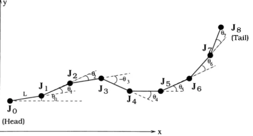
In our work, we will deal with a similar structure except that our structure is composed of eight links of the same length and for each link, a link-solenoid is assumed to be able to fix the entire link to the surface. The last assumption can be realized by using a solenoid pair for each link. For motion planning purposes, the structure can be simplified as in Figure 3.1. Each segment is represented by a line segment of length L. Joints and segments are ordered beginning from the head so that Joint 0 is the head joint. Joint 8 is the tail joint. Segment 1 is the head segment and Segment 8 is the tail .segment. Joint i is denoted bj'

Ji for i = 0,1, ...,8. Let us denote the ray Ji-iJi hy Li for ?’ = 1, ...,8. .Joint angles

0

state of the solenoid of Segment i for i — where 0 denotes that the segment is free and 1 denotes that it is fixed by its solenoid.

J s (Tail)

Figure 3.1: Simplified structure of the mechanical .snake.

To avoid possible needs to apply large amounts of torque to swing big portions of the mechanical snake and to avoid a jack-knifed situation, in which the snake is bent over an intermediate joint and motion control is very difficult, absolute values of the interior joint angles O

2

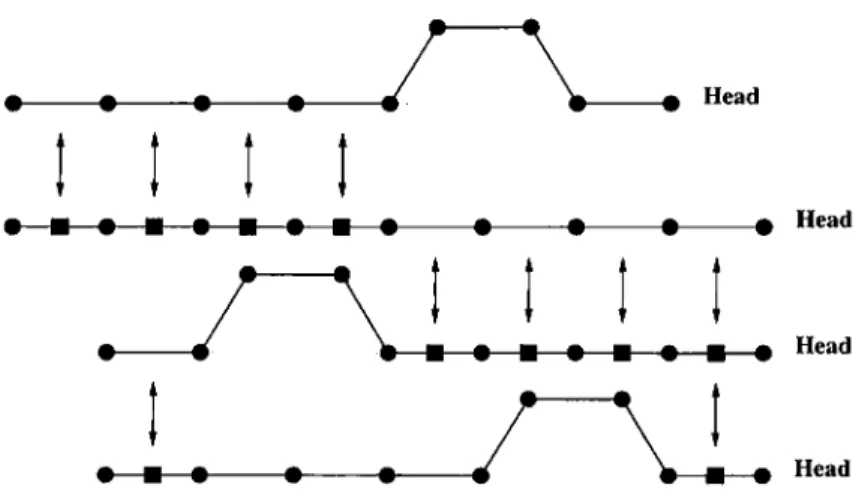
Based on the structure and the angle-constraint given above, the basic linear motion pattern is as follows:

Step h h Ox (^25^3

0

67

1 0 0 1 1 0° 0° 0° 0° 0°

2 1 1 0 0 0° 0° -6 0 ° 60° -6 0 °

3 1 0 0 1 -6 0 ° 60° -6 0 ° 0° 0°

Head - ·--- · --- · --- · --- · ' A A ' · ' ■ · --- · --- · --- · · ■ · Head Head Head Figure 3.2: Basic linear motion pattern.

This pattern can be easily generalized for cin arbitrary motion which does not violate the constraints. For a general motion pattern, the solenoids which are activated in a specific step will be the same as those activated in the same step of the basic linear motion pattern. .Joint angle changes will slightly differ to move on nonlinear paths. To simplify the general motion pattern, we will adapt a convention that the sequence formed by the three links which are not on the path tracked (e.g. the line tracked for the basic linear motion pattern) is symmetric, that is, the angles of the two joints which are not found on the path are the same.

Using the structure and the motion pattern above, our problem will be to get the mechanical snake out of a rectangular region through a specified exit. The initial configuration of the snake can be arbitrary, but it is assumed that the initial configuration is suitable to follow a smooth path to get out of the region without crashing on the borders.

We specify the problem in order to have an explicit task to deal with:

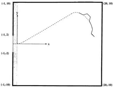
P r o b le m 3.1 Let the length of a segment of the m.echanical snake be normal­

ized to

1. Let the rectangular region of interest, R, be the region having the

corner coordinates (-1, -10), (-1,

10

10

10

be an interval between points (-1, -2) and (-1, 2). Let the mechanical snake

initially be inside the square R{ with corners (0, -

10

10

10

(20, 10). The aim is to take the snake out of R using the specified exit. The

Figure 3.3: Problem 3.1.

This task can be clone in two steps: Generation of the path to get out, and tracking of the generated path by the mechaniccd snake. A separate neural network will be designed to achieve each subtask.

3.3

Generation of Path

To have an unobtrusive motion, and to take steps signilicant in size, the path should be a smooth path with no sharp turns, that is which has a suitable maximum curvature

Kmax-To determine a specific value for the maximum curvature, we will use the angle constraint and two other constraints which nicvke significance of steps explicit. To make the steps of the motion pattern significant, we impose that the distance between J{ and J,+3 is at least 2.8 for a .seciuence Ji+i·, Ji+2i

./¿+3 of joints all of which are on the path to be tracked, and that the distance between Ji and J,+3 is at most 2.2 for a .sequence Ji, Ji+i·, Ji+2·, -A+3 in which

Ji+i, Ji+2 are outside the path to be tracked.

Using the three constraints, the maximum curvature is determined as

Derivation of the maximum curvature from the constraints is given in Ap­ pendix C. Note that further algorithms and neural network structures are in­ dependent of this specific value of Kmax·, il’nd the algorithms can be run and the neural networks can be trained for different minimum radii of curvature by only setting Rmin to the specific value of the minimum radius of curvature.

Suppose that the initial structure is adjusted so that the snake can be represented by a sequence of seven pieces of curves, each of which is either a line segment of length 1 or an arc of radius Rmin and chord length 1 (A neural network to make this adjustment for an arbitrary initial condition will be introduced later). For such a configuration, seven of the joints are at the ends of these curve pieces. Let us order the pieces as Piece 1, ..., Piece 7 from head to tail, and denote the end points of the,se pieces as Vo, ..., V7 in the same order. Let Pi denote both the ray and the type of Piece i for

i - 1,...,7, where the piece-type definitions are given in Figure 3.-4(a). The directional (CCW ) angle from ;c-axis to the ray which is tangent to Piece 1 at Vo and which follows the direction of Piece 1 is denoted by (j>o, and the directional (CCW ) angle from Pi to is denoted by (/)i for i = 1,...,6. Note that the convention used in defining (f)o is different from the convention used in defining

(j)i iov i = 1, ...,6, and Oi for i = 0,..., 7. Using this notation, a configuration

is represented by 10 parameters, position and direction of the head, and types of the seven pieces (xj^, yj^, Oq, Pi, ■■■, P7)· A sample initial configuration, which is represented by {x, y, 180°, —1, —1,1, —1,0 ,1 ,1 ), is given in Figure 3.4(b).

P; = -l :

Vi V,,

P,= 0 : · --- ^

P;= 1 :

Figure 3.4: (a) Piece-type definitions, (b) The initial configuration represented by {x, y, 180°, - 1 , - 1 ,1 , - 1 ,0 ,1 ,1 ) .

Ri ending at the origin with a direction perpendicular to the exit interval. After that point, linear motion will be sufFicient to take the snake out. In the realization of the task, the path generated will not exactly end at the origin with the specified direction, but these values will be close enough to the desired ones to exit from the specified interval.

So, the path generation problem Ccin be formulated as finding a path X {t) —

{x{t).,y{t)) in the right half plane such that AT(0) = </’(0) = A’ ( i /) = 0

cind = 180° for some tf, and n{t) < Kmax·, Vi G [0, i/]. Here, <^(i) = atan2(?/(i), ."¿(i)), where atan2(.,.) is the signed arctan function, defined .same cis the (7·^·*· comnicind atan2, and K{t') is the curvature of the path X {t) at

t = t'.

This ¡problem will be approached in two different ways, and two different neural networks will be designed for path generation in the next two chapters. Both of the paths generated using these two approaches will be compositions of the three arc types defined above, with smooth connections. Path generator neural network can be represented by the block given in Figure 3.5, for both approaches.

y

0

Figure 3.5: Path generator neural network.

The inputs of NNpath in the complete neural network will be x = xj^^

y = yjoi ^ — ^0, and the outiDut P' will be type of the next curve piece to be

3.4

Structure of the Complete Controller

The algorithm that will be recilized by the complete controller to achieve the specified task is summarized as follows:

A lg o r ith m 3.1 Given an arbitrary configuration of the snake at an arbitrary

location, represented by the (sensed) variables xj^, yj^, Oi^

0

1. Adjust the initial configuration (

7

pieces of curves representation {xj^^yj^^9o^Pi^...,Pj) is available. 2. While xjq > 0 ;

(a) Using

$0

(b) Apply xjq, yjQ and fio to NNpath inputs to get the type of the next

piece^ P ', as output.

(c) Using 61,

62

7

to be given in the three steps of the motion cycle.

(d) Update the curve piece types as = P', = P\, ■■■,

Prnew = P& 'ieari step.

(e) Realize the 3-step motion cycle using the joint angle increments ob­

tained in Step

2(c).

(f) Get new values of xj^, yj^, Oq, 0\, ..., 0-j using sensors.

3. While x j^ > —I :

(a) As.sign the type of the next piece to be tracked as P' = 0.

(b) Apply steps

2(d),

2(e) and 2(f).

4. Stop.

The task is accepted to be finished, when the head of the snake is departed from the region R. Consequently, a path consisting of the same three types

of curve pieces which is suitable for the environment can be generated for controlling the motion outside the region.

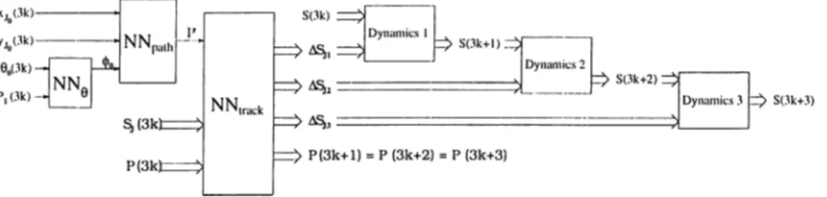
A neural network to adjust the initial configuration will be directly designed in the last section of this chapter. The complete neural network controller scheme for the adjusted initial configuration is given in Figure 3.6. Vector variables in this scheme are defined as follows:

,9 I/Jq·) ^0? ^1? ···? ^7] (3.1)

= [«., »2, .... D rf (3.2)

P = [i>„ f t , P r f (3.3)

A S ji, ASj

2

1, 2 and 3 of a motion cycle.

Figure 3.6: Complete neural network controller scheme for the adjusted initial configuration.

The blocks Dynamics 1, Dynamics 2 and Dynamics 3 simply realize the Steps 1, 2 and 3 of a motion cycle. That is, Dynamics i activates the solenoids for Stei? i according to Table 3.1 and forces the joint motors to apply the increment ASji, for i = 1, 2, 3. The neural network blocks NNtrack and

NNg will be described in the next section. They are designed to implement Steps 2(a), 2(c) and 2(d) of Algorithm 3.1.

3.5

Tracking the Generated Path

The neural network block NNtrack is designed to get the joint angle increments to be given in the three steps of the motion cycle, using Oi,

62

7

..., P7, P ' , and to update the curve piece types for the next cycle.

We will use the two facts expressed below to design this block. Proofs of these facts will be given in Appendix B.

Fact 3.1 I n a n y c o n f i g u r a t i o n , v a l u e o f (f)i i s g i v e n b y

(3.4)

f o r i = 1, ..., 6, i v h e r e t h e c o n s t a n t f i i s d e f i n e d a s

/3 = arcsin 1

2 Rinin (3.5)

Proof: See Appendix B. □

Corollary 3.1 F o r a c o n f i g u r a t i o n w h e r e S e g m e n t s i a n d i + 1 l i e o n ( h a v e t h e s a m e e n d p o i n t s w i t h ) P i e c e s k a n d A: + 1, t h e j o i n t a n g l e O i i s g i v e n b y

— —/3{PkPPk+i) (3.6)

w h e r e ( 3 i s d e f i n e d b y E q u a t i o n 3 . 5 .

P r o o f: For such a configuration, Ji, Ti+i, Oi coincide with 14-1, 14, I4+1,

fk respectively, and the result immediately follows. □

Fact 3.2 F o r a c o n f i g u r a t i o n w h e r e J i - i , J i , J i+ 3 a n d . I i+ 4 c o i n c i d e w i t h 14-i,

14

14

2

14+3

^,+3

^¿+1 Oi Oi+3 -- Oi.A.2 —_{i+ 2 = «|Pfe+i+p^.+2l (3-7)} - l 3 ( P k +

2^k+l + 7yPk+2) -

+2

2)

+2

Proof: See Appendix B. □

The choice among the two candidates given in Fact 3.2 will be based on the joint angle constraint. To guarantee that the absolute Vcilue of the interior one of 9i and ^¿4-1 is below 63°, the choice in which the sign in front of the o-term is opposite to the sign of the rest of the expression for that angle will be selected.

Based on this selection rule in addition to Fact 1 and Fact 2, the values of joint angles for a cycle with A^A^iracfc-hiputs Of^., 0^'^ •••i ^7'^^ P\i P2·, ..->^7, P '■,

Joint Angle Initial After Step 1 After Step 2 After Step 3 Ox QO^ld Qi Qi Ql + Q2/2 — S20lk2 ^2 Q2 Q2 S20Ck2 ^3 Qold Q3 Qs S20ik2 Ox Q‘i Q‘\ + <3.5/2 — Q3 + Q2/2 — S20Lk'2 06 Qold SlOfu Qa 0e 0°‘^ 0°‘<^ SxCXki Qr)

07 Qold Qe + <3.5/2 — sjaA,., <3e Table 3.2: Joint angles during a general motion cycle.

Here Qi, .si, .S2, and k

-2

Q г = -^ (P ' + Pi) (3.14) Q i - - / 3 { P i - i + P i ) f o r ¿ = 2,3,4, .5,6 (.3.15) s x = sign((34 + <3.5/2) (.3.16) h = \ Q 6/ I ^ \ (3.17) S2 = Sign((33 + Q 2/ 2) (.3.18) h = \ Q 2l P \ (3.19)

where sign(.) denotes the function of a bipolar hardliiniter defined as:

sign(,T) - 1 , .t: < 0 1 , x

> 0

(3.20)

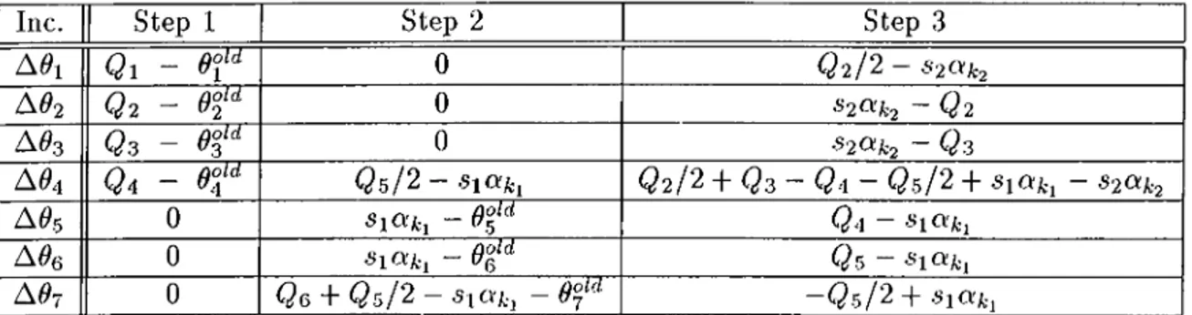
So the joint angle increments to be applied during a cycle are obtained iis given in Table 3.3.

Having the table for angle increments, we can now design the NNtrack

circuit. Collecting Q i, ..., Qe in vector Q and the new piece types P„i, ..., Pn7

Inc. Step 1 Step 2 Step 3

Q i - 0 <_{3 2 / 2} - S₂CVfc₂

A O 2 Q 2 - d°2“‘· 0 ~ Q2

A^3 Q z - e r 0 S20ik2 - Q z

A 0 4 _Qa - 04"" Q s / 2 - sittki <3 2 / 2 + <33 - <3-1 - <3.5 /2 + - S2«A;2

A05 0 SlOiki - 0 t ‘ '^ <34 — SlOiki

A06 0 s i a k , - 0 t ^ _<3s

-A 0 7 0 Q e + Q5 /2 - s ia u , - 0°r‘ ^ —Q r j 2 + s\aki

Table 3.3: .Joint angle increments during a general motion cycle.

Q — [Qi·, Q2, ·■·, Qe]^

Paew — \Pn\i Pn2t •••1 Pn7]

N Ntrack can be divided into subblocks as pictured in Figure 3.7.

(3.21) (3.22)

P’

Figure 3.7: N Ntrack ■

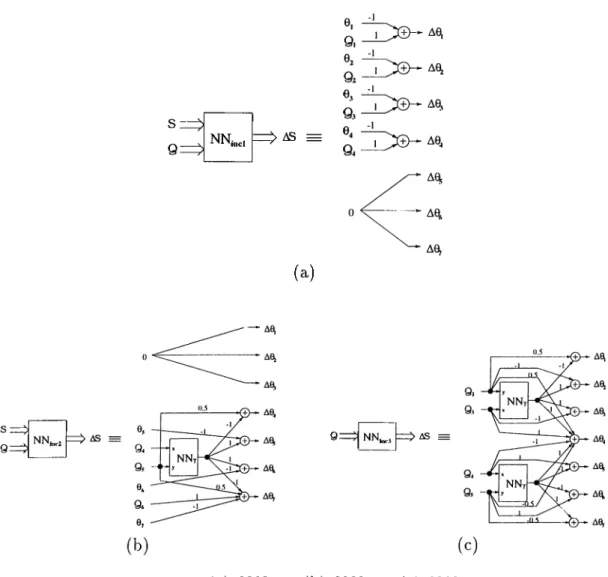
Here, NNconv is used for deriving the vector Q from P and P'. NNupdate

updates the vector P for the next cycle. NNinci, NNinc2 and NNinc:i compute the increments to be given to the joint angles in Step 1, Step 2 and Step 3 of the current cycle respectively.

In the rest of this section, neural network structures of these sul)blocks and structure of NNot which is used to obtain will be given. The activation functions used in these blocks are unipolar and bipolar hardlimiters. Note that each one of these two types can be constructed as a simple neural network with a single activation function block of the other type. So one type of activation block is sufficient to construct the subblocks of

NNtrack-NNupdate and N N c ,conv ·

P’---- > NN._updiilt' P .. = P' P| P2 P, P. P5 p. P„. P..4 P„5 P„. p». (a) (b)

Figure 3.8: (a) NNupdate· (b) NNc,

N N inel, N N inc2 and N N in cr-

Let us define a function j{ x , y) as

9, 92 9, 9a a 9. 7(.T, y) = sign[x + y l

2)a\y/p\

1

7(0;, y) will be implemented by the neural network N N^^ whose structure will be described later. The structures for NNinci, NNinc2 and NNi„,c3 includ­ ing NN^ are given in Figure 3.9.

S z ;

9 = ^ NN,.„ ^ =

(a)

Si

9 = NN,„ NN...

Figure 3.9: (a) NNinc\- (b) NNinc2- (c)

NNincs-N NNincs-N ^ .

This block is designed as shown in Figure 3.10(a), where the block NNa

will be designed to implement the function

N N a :

This block is designed as two subblocks, NNai to implement

a i(a ) = |a|

fo r a € { —2, — 1 ,0 ,1 ,2 } and to iiTiplement

CV2(«, b) = a ab

for a € { — 1,1} and b € {0 ,1 ,2 }. a

2

(3.26)

(3.27)

a - 1 - 1 - 1 1 1 1

b 0 1 2 0 1 2

0

2

Table 3.4: Possible input-output pairs for N Na2-

NNai and NNc

2

N Ny N N .I NN« (a) b— (b) NN„ NN„ NN„ X—HNN„,h^o = X , b > (c ) (d)

NNe:

This neural network is used to obtain using 0q and Py.

Thinking (/>0 as the direction of an extra curve piece of type 0, and using Fact 1, the difference between the angles </>o and 0q is found as:

(j

>0

Using this fact, the neural network is designed as in 3.11 where NN,nod is used to keep the output in the interval [0, 27t).

H p,- NN.

(a) (b)

Figure 3.11: (a) NNe. (b) TV iV w

3.6

Adjusting the Initial Configuration

Supposing that the initial configuration is sufficiently smooth with representa­ tive curve with maximum curvature close to «max, we developed an algorithm to adjust the configuration so that the representative curve is converted into a secpience of curve pieces of specified types, which is very close to the initial one. Adjustment will be done in one motion cycle:

Algorithm 3.2 Given an arbitrary initial configuration of the mechanical

snake with joint angles

0

0

1. A05 = A0e = A07 = P

2

3

2. If 0f^^ < - 60° - f , then P4 = 1, A02 = 60° - 0^^, A0^ = 60° - 0 f \ A04 = 60° /3

-else if -6 0 ° - f < < - 60° + f, then I\ = 0, A(?2 =

A6»3 = 60° - A6>4 = 60°

-else if -60° + f <

0

-else if 0° < < 60° - f , then /i, = 1, M

2

3

else if 60° - f < < 60° + f , then P4 = 0, A02 = -A(?3 = - 60° - A^4 = 60° - Of^;

else if > 60° + f,theni^i = - 1,A^2 = - 6O °-0^ '^ A03 = Aft, = 60° + /? - ftf^'; 60° - 60° - 60° - 60° - of^·, - 60° 3. If < - 60° - f , then P i = 1, A6>1 = - 60° - /? - e f'^ ;

else if -60° - f < < - 60° + f , then Pj = 0, A^i = 60° -else if -60° + f < < 0°, then P, = 1, A^j = _ 60° + /3 -else if 0° < 0 f ‘ < 60° - f , then P, = 1, A6>i = 60° - /3 - O f ;

else if 60° - f < 0i‘‘^ < 60° + f , then P, = 0, A^, = 60° -

elseiief^ > 60°+ f , then Pi = - 1, A^j = 60° + /3-0l‘^.

4. Apply Step 1 of the motion cycle. 5. A^i = A 0 2 = A 0 3 = A 0 4 0

6. Fori = 2,3,4:

I f6>?|‘^3 < - f - P,+2^, then P,-+3 = 1, A6>i+3 = - (P,+2 + l)/3

-else i f - f - Pi+2/? < i'f+s < f - Pi+2^, then Pi+3 = 0, A ft+ 3 =

-P.+2/3- ^ f l i ;

elseif^ f| ''3 > f - Pi+2/?, then Pi+3 = - 1, A^i+3 = - (Pi

+2

7. Apply Step 2 of the motion cycle.

9. Apply Step 3 of the motion cycle.

Based on this algorithm, the scheme for the adjustment of the initial con­ figuration and the neural network structures used for adjustment are given in Figures 3.13 and 3.14. To illustrate the algorithm, a sample adjustment process controlled by these neural networks is pictured in Figure 3.12.

.1..1.. i... i ! i Th(?taI2J=i-60.00 Theta[31 =1-60.00 Thatat4I =r 4t*08 ThetaC71=:-15.75 Head tn>78.. 543 hetaCO] = 205.20 hetaEl] = 47.08 ieta[21 = hetat3] = [4] = letaL.. ieta£5I letaCei , hetaC7] = -12.92 'Head =11.78, 5.13 60.00 -60.00 47 08 0.00 0.00

S(-3) : NN,_{udJI i>P(-2)} t>a-2): Dynamics 1 S " ^ ASj NN.iidJ2 Dynamics 2 z ^ R - l ) =P(0) |=> S(-l) : 4^,= 0: :ii> S(0) Dynamics 3 a A0, Pni A04

(b)

Figure 3.13: (a) The scheme for the adjustment of the initial configuration.

NN„ > P

-Chapter 4

MINIMAL PATH APPROACH

In the ])ath generation task, our aim is to design a neural network to find a path in Ri ending at the origin with a direction perpendicular to the exit interval. In the realization of the task, the path generated will not exactly end at the origin with the specified direction, but these values will be close enough to the desired ones to exit from the specified interval. In Section 3.3, the path generation problem was formulated as finding a path X{ t) = {x{t),y{t)) in the right half plane such that X (0 ) = Xq, ф(0) = фо, X ( t f ) = 0 and ф{і/) = 180° for some tf, and к{і) < Ктах, Vi G [0, t/].

The design in this chapter will be based on finding such a path which has the minimum possible length. First, an algorithm to find the minimum path will be given. Then, this algorithm will be used to train a multilayer neural network used for path generation.

4.1

Minimal Paths on the Right Half Plane

The general problem of finding minimal-length smooth paths with bounded curvature on a region in with or without obstacles is attacked by many researchers. This problem can be formulated as follows [24]:

P r o b le m 4.1 Let ft C 6e « dosed set of polygons representing the obsta­

cles, and let dfl and int(ii) denote the boundary and interior of Ll respectively.

Let us consider the class of paths X( t ) — {x{t),y{t)) G satisfying the

constraints: A'(0) = IP, ФІО) = Фо, 3tf > 0, such that = FP, ф(і/) = ф/, X( t ) e R2\int(Q), Vi G [0 ,i/], l|A(i)ll =

^/(x

t) + y

t))

where Rmin is the m,inimum. acceptable radius of curvature, IP is the initial point and F P is the final point. The problem is to find a path X*{t) defined

f o r t e [0,i}] such that Fj is minimum among tjs of all paths in this class.

Our region of interest is obstacle-free, that is if = 0 in our case. The forms of the minimal length paths for this case were determined by Dubins [24, 25]:

T h e o r e m 4.1 [25] Every minimum length planar curve satisfying the condi­

tions о / Problem 4.1 with Ll — 0 is necessarily a curve which is either

1. an arc of a circle of radius Rmin followed by a line segment, followed by

2. a sequence of three arcs of circles of radius Rmin 3. a subpath of a path of either of these two h

Our algorithm to find minimal paths on the right half plane will be based on this theorem. Paths of Form 2 rarely occur. In our ca,se, since the final point

F P is the origin and fit/) = 180°, and the initial point IP .should be in the right half plane, the rate of occurrence of Form 2 is much smaller. Furthermore

these paths can be replaced by slightly longer paths which are unions of two paths of Form 1 or Form 3. Because of these facts, dealing with only Forms 1 and 3 will not effect the result much whereas the algorithm will be simplihed.

Since we are looking for a path of Form 1 or Form 3 of 4.1, this path can be either:

1. an arc of a circle of radius Rmin followed by a line segment, followed by an arc of a circle of radius Rm in (Form 1)

2. an arc of a circle of radius Rmin followed by a line segment

3. a line segment followed by an arc of a circle of radius Rmin

4. an arc of a circle of radius Rmin followed by another arc of a circle of I’cldiuS R m in

5. an arc of a circle of radius Rmin

6. a line segment

If we let the arcs and the segment to have length 0, the first case will include the other cases. For example, a path of Case 4 can be thought as an arc of a circle of radius R m in followed by a line segment of length 0, followed by an

arc (5f a circle of radius R m in· Furthermore, the path should completely lie on

the right half plane. The algorithm will define these three curve pieces and the command sequence to follow these curve pieces, if such a path exists. If there is no such path cind if there is a directed arc in the right half plane beginning at IP with tangential direction фо and ending with tangential direction 0°, this arc will be followed, then a line segment will be followed till reaching a point IP ' for which a minimal path composed of three curve pieces exists. The tangential direction at IP ' will be eventually 0°.

The output of the algorithm will be a sequence of five parameters defining the path: CPi, CP5. If a minimal path exists, CPi = CP

2

C P5 indicate the angles to be proceeded on respectively the first and the second

arc (the third curve piece). Signs of CP3 and CP

5

length of the line segment (the second curve piece) of the path. If a minimal path can be found after maneuvering as described above, CP\ and CP2 are the parameters for the arc and the line segment proceeded for steering to a point for which a minimal path exists. CP3, CP.i and СРг) ai'e defined the same as the case of existence of a minimal path. Signs and values of CP\ and CP2 have the same indications as CP3 and CP^ respectively. If there is no such path, all of the five parameters are 0.

Given IP = {x, y) and фо = 0, there are two circles with radii Rmin

tangent to the ray originating from I P with inclination в. Let us denote the circle on the left of the ray by РС( х, у, в) and the one on the right by

R C ix, y, в). Similarly, there are two hxed circles tangent to the ray originating

from P'P = (0, 0) with inclination 180°. We will denote the one on the щэрег half plane by FCi and the one on the lower half plane by F C

2

-So, given IP — (x, y) and фо = 61, if a minimal path exists, the first curve piece will be an arc on either LC(x^y,9) or РС( х , у , в ) , the third piece will be another arc on either FC\ or F C2, and the second piece will be a line segment tangent to these arcs. Moreover the orientation of motion can only be CCW on LC{ x, y, 0) , CW on RC( x , y , e ) , CW on FCi and CCW on F C

2

Given two circles C\ and C2, there are at most four line segments which are tangent to both of the circles (having end points on the circles). Orientation pair of arcs of a smooth path containing one of these line segments on and

C2 is different from that for another element of the set of tangent line segments. So given one of the oriented initial circles РС( х, у, в) and RC( x, y, 0) , and one of the oriented final circles FCi and F C

2

Let us consider LC{x,y^0). If it is in the lower half plane, a minimal path having its first arc on this oriented circle can not have a portion on FCi. If

LC{ x, y, 0) intersects with the right half plane, a path having its first piece on

LC( x, y, 0) and its last piece on F C

2

candidate for a minimal path having its first piece on LC{x, y,0).

By symmetry, the same fact is valid for also RC{ x, y, 0) . That is there is at most one candidate for a minimal path having its first piece on RC{x, y, 0).

So for given I P = (x, y) and (¡)q = there are at most two candidates for a minimal path, one having its first arc on LC{ x, y, 9) and the other having its hrst arc on RC{ x, y, 0) . A sample situation is given in Figure 4.1. In this situation, thei’e are two candidates for the minimal path; Path 1 and Path 2. The shorter one. Path 1, is the desired minimal path.

F’igure 4.1: Minimal path candidates for I P — (x, y) and (j)Q = 0.

Based on these facts and some further analysis, we have developed the algorithm given below. Location of LC( x, y, 0) and RC{ x, y, 9) , and the cases in the algorithm are illustrated in Figure 4.2 and Figure 4.3.

A lg o r ith m 4.1 Given an initial point IP = (.r, y) and initial direction <f>o = 0: