Genetic neural networks to approximate feedback Nash equilibria in dynamic games

(1)

Computers Available at

www.ElsevlerMathematics.com

An International Journal

computers &

mathematics

with

applicatha and Mathematics with Applications 46 (2003) 1493-1509

www.elsevier.com/locate/camwa

Genetic

Neural

Networks

to Approximate

Feedback

Nash Equ,ilibria

in Dynamic

Games

S. SIRAKAYA*

Departments of Economics and Statistics and Center for Statistics and Social Sciences University of Washington, Seattle, WA 98195-4320, U.S.A.

sirakayabstat.washington.edu

N. M.

ALEMDAR

Department of Economics, Bilkent University, 06800 Bilkent, Ankara, Turkey

alemdar@bilkent.edu.tr

(Received October 2001; revised and accepted June 2003)

Abstract-This paper develops a general purpose numerical method to compute the feedback Nash equilibria in dynamic games. Players’ feedback strategies are first approximated by neural networks which are then trained online by parallel genetic algorithms to search over all time-invariant equilibrium strategies synchronously. To eliminate the dependence of training on the initial conditions of the game, the players use the same stationary feedback policies (the same networks), to repeatedly play the game from a number of initial states at any generation. The fitness of a given feedback strategy is then computed as the sum of payoffs over all initial states. The evolutionary equilibrium of the game between the genetic algorithms is the feedback Nash equilibrium of the dynamic game. An oligopoly model with investment is approximated as a numerical example. @ 2003 Elsevier Ltd. All rights reserved.

Keywords-Feedback Nash equilibrium, Parallel genetic algorithms, Neural networks.

1. INTRODUCTION

This paper proposes a new method that can efficiently offer highly accurate approximations to feedback Nash equilibria of dynamic games which lack explicit solutions. We focus on feedback perfect state information pattern and parameterize each feedback rule by the weights of a suitable neural network, thereby transforming the players’ strategy spaces from a set of rules to a set of neural net weights. For each network, an artificially intelligent player, a genetic algorithm (GA).

is assigned to breed fitter weights and update other GAS via the computer shared memory as to its best-to-date feedback rule.

In any given generation, the game starts from a fixed set of initial states. Since we are searching for the stationary feedback rules, the same neural net weights are used to compute the payoffs. The raw fitness of a potential feedback rule is then calculated as the sum of all payoffs across all initial states. Our rationale for repeating the game from multiple initial states is two-fold: to

*Author to whom all correspondence should be addressed.

(2)

1494 S. SIRAKAYA AND N. M. ALEMDAR

avoid the dependence of the weight training on the initial conditions and also to speed up GA learning.

In essence, each GA trains a neural network online to best respond to the other players’ best feedback rule in the previous generation. Initially, GAS start a blind search. However, as the search progresses, each player’s network is trained to incrementally best respond to any policy rule of the others. The fittest weights are then communicated to each other via the computer shared memory. Equipped with the updated weights, each player is better able to anticipate the best response of the others for all potential rules in its population. The individuals that exploit this knowledge to their advantage are fitter, thus, reproducing faster. Ultimately, the fitter weights dominate respective populations also steering the other players’ search for the best set of rules to the vicinity of the feedback Nash equilibrium.

The feedback Nash equilibrium is a desirable solution concept because, by definition, it is

time-consistent. Unfortunately, however, feedback solutions are often analytically intractable.

Explicit solutions are restricted to a class of special cases, for instance, a linear quadratic game where objective functions are quadratic, laws of motion are linear, and control variables are

unconstrained. For problems with nonlinear function specifications and constrained decision

variables, on the other hand, linearly parameterized numerical approximations, such as spline functions or radial basis functions (RBFs), are frequently employed. Other dynamic programming techniques which rely on the approximation of the Bellman equation are also often used. As the state space gets larger, however, the aforementioned methods quickly become unmanageable due to exponentially rising computer memory requirements also known as the curse of dimensionality. The proposed method in this paper is free of the so-called curse of dimensionality as both GAS and neural networks are inherently parallel structures thus are highly efficient users of computer memory.

The balance of the paper is as follows. In Section 2, we briefly discuss the concepts and solutions involved in dynamic games. Section 3 first presents a short overview of the neural networks and genetic algorithms, and then proceeds to show how, parallel neural genetic algorithms can approximate the feedback Nash equilibria. Section 4 tests the algorithm on the dynamic oligopoly game provided in [l]. Conclusions follow.

2. DYNAMIC

GAMES

AND

SOLUTION

CONCEPTS

For presentational simplicity, consider the following generic two-player finite-horizon dynamic game in discrete time, t E T. For players, i = 1,2, let the mi-dimensional state, zi E Xi c R”;, evolve according to’

x;+~ = F; (z,1, x,2, u;, ut”) , xfj is given, ₍₁₎

and where uf E Vi c 7P denotes the ni-dimensional control vector for t = (0, 1,2, . . . , T - l}. Given any strategy of the other, player i chooses his strategy to maximize the objective functional

T-l

Ji (u1,u2) = c Rf (2~+,,,~2,2t2+~,~~,21:,2~t2). t=o

The terms open-loop and closed-loop refer to the information structures in dynamic games.

In the former case, players’ information sets consist of the initial values of the state variables and time so that right at the beginning of the game, players announce and commit themselves, with no possibility of update or alteration throughout the game, to a path of controls which are functions of time and the initial states, ui = {zJ:(x~)}~&‘. The relevant equilibrium concept in this class of strategies is referred to as open-loop Nash equilibrium. Open-loop Nash equilibria are only weakly timeconsistent and therefore, in general, not subgame-perfect2

‘For numerical computation, infinite-horizon differential games can be discretized as in [2] so that the discussions that follow can be extended without any loss of generality.

(3)

Genetic Neural Networks

Note that by recursive substitution of equation (1) into (2)> the objective functionals drpenc! only on controls and the initial states

(3,

Thus, a pair of open-loop strategies, (ul*, u2*), constitutes an open-loop Nash equilibrium of the game defined in equations (1) and (2) if and only if

J1 (ul*, u2*) 2 J’ (u’ ) u2*) ,

$2 (d*, u2*) 2 J2 (d* , u”) , iJi

for all permissible .open-loop strategies u1 and u2.

The above inequalities mean that given the initial date and state, each player’s precommittetl action path constitutes a best, response to other players’ chosen paths. However, this may not be true for the continuation of this strategy when viewed from any other intermediate time and state. Thus, in general, equilibrium policies generated by the open-loop decision rule are not subgame-perfect.

Under the closed-loop information structure, players’ strategies may depend on the whole

history of the dynamical system. Players do not precommit but revise their decisions as new information becomes available. Information sets of players in this case may consist of the valurs of state variables up to the current time (closed-loop perfect state information pattern). the,

initial and current values of the state variables (closed-loop memoryless information pattern) or the current values of the state variables (feedback perfect state information pattern). The> relevant equilibrium in this case is called the closed-loop Nash equilibrium. In general, a plethora of closed-loop Nash equilibria exist when the information structure for at least one player is dynamic and involves memory [S]. In this case, the Nash equilibrium concept can be refined b, requiring it to be subgame-perfect. Such an equilibrium is called a feedback Nash equilib~-ium.

In this paper, we focus on equilibria that are subgame-perfect, the so-called feedback Nash equilibria. Feedback Nash equilibrium is defined by inequalities (4) with the added requirement that they hold for all time and state pairs. Requirements for the feedback Nash equilibrium ~LIV compatible with any information pattern in which all players have access to the current value of the state variables [8]. However, in order to narrow t;he search space, we restrict ourscivc,s to the feedback information structure and focus on time-invariant feedback rules. Thus, a cont,roi law, y’, for player i is a function of the current, state of the system

u; = yl (xt’J$)

(5 i

A pair of closed-loop strategies (y1*,y2*) is a feedback Nash equilibrium of the game defined iI1 equations (1) and (2) if and only if

J1 (y1*,y2*) _{2 J’ (-$,r”*)} ₃ 7 (yl*, r”*> 2 7 p/l*, r2) 1

for all admissible closed-loop strategies y1 and y2.

3. A BRIEF

NOTE

ON NEURAL

NETWORKS

AND

GENETIC

ALGORITHMS

((8

We approximate players’ feedback rules by feedforward neural networks which are then trained online synchronously by genetic algorithms in a parallel manner to search over all time-invariant equilibrium strategies. Neural network specification offers some advantages over the traditional

(4)

1496 S. SIRAKAYA AND N.M. ALEMDAR

techniques, such as spline functions or RBFs. First, feedforward neural networks have been proven to be universal function approximators in the sense any L2 function can be approximated arbitrarily well by a feedforward neural network with at least one hidden layer. (See, for example, [9,10].) Second, nonlinearly parameterized nature of feedforward neural networks allow them to use fewer parameters to achieve the same degree of approximation accuracy as opposed to linearly parameterized techniques which require an exponential iocrease in the number of parameters. Third, neural networks with sigmoid activation function at the output layer naturally deliver control bounds, while such bounds constitute a major problem for linearly parameterized techniques. Fourth, neural networks can easily be applied to problems which admit bang-bang solutions, while this constitutes a major difficulty for other conventional methods.

There are several good reasons for our choice of genetic algorithms to train the neural networks

as well. First, as opposed to the gradient-descent methods, genetic implementations do not

use the gradient information. Thus, they do not require the continuity and the existence of derivatives of the objective functionals and state transition functions. The only restrictions are that they be bounded. Naturally then, our method can be applied to a larger class of problems. Second, GAS are global search algorithms which start completely blind and learn as the game unfolds. Regardless of the initial parameter values, they ensure convergence to an approximate global optimum by exploiting the domain space and relatively better solutions through genetic

operators. Gradient-descent methods, on the other hand, need gradient information and may

stuck in a local optimum or fail to converge at all, depending on the initial parameters.

3.1. Neural Networks

Neural networks are information-processing paradigms that mimic highly interconnected, par-

allelly structured biological neurons. They are trained to learn and generalize from a given set of examples by adjusting the synaptic weights between the neurons.3

Consider an L layer (or L - 1 hidden layer) feedforward neural network, with the input vector z” E RTo and the output vector 4(z”) = zL E 7VL. As in [ll], we refer to this class of networks as n/T”,,, I,..., TL’ The recursive input-output relationship is given by

yj = w3z3-1 + .j 7 (7)

where the connection and the bias weights are, respectively, w = {wj, d}, with wj E RTj xrj-l and ujE77-j forj=1,2,... , L. The dimension of yj and tj is denoted by rj. The scalar activation functions, gj(.) are usually sigmoids, e.g., gj(.) = tanh(:) or aj(.) = l/(1 + exp(-(.)) in the hidden layers. At the output layer, the activation functions, a~(.), can be linear, e.g., go = (.), if the outputs have no natural bounds. If, however, they are bounded by 0min 5 zL 5 emax, then one may choose

OL (.) = &in +

e max - 4nin

1 + exp (- (.))’ (9)

Thus, the approximating function has the general representation

dJ (~“+J) = CL (WLBL-I (wL-leL-2 (. . . (w% (w’c + w’) + 2) + v”) +. . . + vL-1) + VL). (10)

3.2. Genetic Algorithms

The neural networks in our game algorithm are trained online by parallel genetic algorithms. That is, the interconnection weights between the neurons are incrementally adjusted by synchronous parallel GAS. A basic GA consists of iterative procedures, called generations. In each

3For the sake of compactness, the notation this section closely follows [ll]. A well-documented theory of neural networks can be found in [l&13].

(5)

Genetic Neural Networks 1497

generation, say s, a GA maintains a constant size population, Pop(s), of candidate solution vectors to the problem at hand. Each individual in Pop(s) is coded as a finite-length string, usually over the binary alphabet ((0, 1)). The initial population, Pop(O), is generally random.

At any generation, each individual in a population is assigned a ‘fitness score’ depending OII how good a solution it is relative to the population. During a single reproduction phase, relative11 fit individuals are selected from a pool of candidates some of which are recombined to generate> a new generation. Better solutions breed faster while bad solutions vanish. Basic recombination

operators are mutation and crossover.

Crossover randomly chooses two members (‘parents’) from the population, then creates two similar off-spring by swapping the corresponding segments of the parents. Crosso+er can b(x

considered as a way of further exploration by exchangin, 6 information between two potential

solutions. Mutation randomly alters single bits of the bit strings encoding individuals with IL probability equal to the mutation rate pmut. It can be interpreted as experimenting to brceti fitter solutions.

GAS are highly parallel mathematical structures. While they operate on individuals in a

population, they collect and process vast amounts of information by exploiting the similarities in classes of individuals, which Holland [14] calls schemata. These similarities in classes of individuals are defined by the lengths of common segments of bit strings. By operating on r~ individuals in one generation, a GA collects information approximately about n3 individuals [14].

Parallelism can be explicit as well in the sense that more than one GA can generate and collect data independently and that genetic operators may be implemented in parallel (see [15]), Parallel genetic algorithms are inspired by the biological evolution of species in isolated locales. To mimic this evolutionary process, a population is divided into subpopulations and a processor is assigned to each to separately apply genetic operators while allowing for periodic communication between them. Subpopulations, specialize on one portion of the problem and communicate among themselves to learn about the remainder. We exploit this idea in training the neural networks t,o approximate the feedback Nash equilibria.4

3.3. Approximation of Feedback Nash Equilibrium with Genetic Neural Networks

For training the neural networks, we propose the following algorithm. First, parameterize the feedback control law of player i in the game given by equations (1) and (2) by a neural network as

where 2,” is the time t input vector to the network approximating the feedback control law of player i. It is an ro-dimensional vector of the state variables at time t, such as 2: = (z,‘, 2;) or Zt ’ = (z,‘, z,‘, z$). Note that the neural network architectures chosen to approximate the feedback rules of Player 1 and 2 and/or their input vectors may not be the same, depending on the game. For notational simplicity, however, we assume here that the input vectors for both networks are the same. Next, for each player i, use equation (11) in the state transition equation (1) to get

xi+1 (thus, z:+~) as

2% _t+l _{= F,i} _@‘(db’) _d2 _(db”) _dd): (12)

where xi E Xi is given. Substituting equation (11) and recursively substituting equation (12) into (2), we have

T-l

si (LJ,c2) = c Pt _{( x&x&} _$’ _(ZIP’) _{1 42 (z10,w2>>} _. t=o

41n [2,16], parallel GAS are employed to approximate open-loop Nash equilibrium in discrete and differential games, respectively. In [17], GA parallelism is used to compute the Stackelberg equilibrium in sequential games.

(6)

Note that given the initial states, the strategy spaces of the players are now transformed from a set of rules to a set of neural net weights. Therefore, the weights of the networks can be adjusted to maximize each player’s respective payoff given the weights of the other. The ability of the networks so trained to generalize, however, will be limited as the training depends upon the initial conditions of the game.

Thus, our next task is to devise a method so that the trained networks can generalize over a wider set of initial states. Towards that, we note that if a stationary feedback policy of a player maximizes its respective payoff for any given initial state, then it must also maximize the sum of payoffs over a set of initial states. Defining a set of initial states as II c Xi x Xi, for any given

set of weights and initial states, (zh, ~1) E II, we can generate the sample paths for the states (thus, the input vectors at any time t E [0, T - 11) and feedback policies from (11) and (12), as MEk and {#(.zF, w”)}&c’, respectively. Thus, the sum of payoffs over all initial states is

T-l

ji bJ+? = c Criz’(&-&q+ ($,wl) ,@(&d2))~ (14)

(x&c;)En t=o

Hence, if the neural nets approximating the stationary feedback policies are trained so as to maximize this sum, then they will have a better generalizing capacity.

In passing, we note that many neural networks can parameterize the feedback rule yi(xi, x:), There exists no hard-and-fast rule of choosing a network architecture other than a systematic trial and error approach. While a network architecture with too many layers and neurons may be very time consuming and may not offer significant improvement over an architecture with fewer layers and neurons, too few layers and neurons may result in poor approximations. As a general rule, simpler architectures are more preferable because they learn faster.

To approximate the feedback rules, we assign GAi to Player i (i = 1,2) to train the neural networks as represented in equation ( 11).5 At any generation s E S, a GA’ operates on a constant size population, Ni, of neural net weights

Popi (s) = {Wf (s) ,&s), . . . ,wg (s) ) . . . ,Whi (s)} ,

where w:(s) E Popi represents a vector of potential weights approximating the optimal feed-

back rule of Player i.

GA1 evaluates each individual b E Pop’(s) by computing its raw fitness,

T-l

ji (w; (s) , w2* _{(8 - 1)) =} _c _c _{R (d, 4k41 (zf, w; (s,) , (f12 (z;, w2* (s - 1))) ,}

(Z&Z$Erl t=o

where w2*(s - 1) stands for the vector of best-to-date weights in the population of GA2 in the previous generation. GA2, on the other hand, computes the raw fitness, j2(w1*(s - l),wj(s)), for each individual d E Pop2(s) g’ iven the best-to-date weights, wl*(s - l), of GA’.

The search is initialized from random populations, Pop’(O) and Pop2(0). Given a random

d E Pop2(0), GA’ finds the best performing individual, b, such that 3 (w:(o) I w; (0)) 2 j1 (w; (0) , w; (4) t

forg=1,2,..., b- 1, b+ 1,. . . , Nl, and updates GA2 with w’*(O) = w;(O). Likewise, GA2 simul- taneously informs GA1 about w2*(0). Next, using the evolutionary operators’, a new generation of populations are formed from the relatively fit individuals, Their fitness scores are recalculated in the light of the previous choices of the opponent, and best performing individuals are exchanged once again.

(7)

Genetic Neural Networks 14Y!'

The above procedures are repeated for a number of generations. That is, at any generation s. GA’ proceeds with the search if there exists a b such that

? (w; (s) , w2* (s - 1)) > 3 (wi (s) ,w2* (s - 1)) *

for g = 1,2,. , b - 1, b + 1,. , Ni. Similarly, GA2 continues the search if there exists a tl sucl~ that

j2 (wl* (s - 1) , W; (s)) 2 j2 (WI* (s - 1) , w; (s)) ,

forg=1,2 ,..., d-l,d+l,..., N2.

As the search evolves, fitter individuals proliferate, thanks to the reproduction and crossover operators, until s’ < S whence for any s > s’, there exist 120 individuals b E Pop’(s) an<1 d E Pop2(s) such that

3 (wl (s) , WC) > ? (wk, w;)

and

P (wk,wi (s)) > 3 (wk,w$) .

where wb and w$ are the weights that best approximates the feedback equilibrium policies. $* and y2*, respectively.

The following pseudocode outlines the steps involved in our parallel GA search for the fecdbac,k Nash equilibrium in a two-player dynamic game.

procedure GA' begin

Randomly initialize Pop'(O);

copy initial weights to shared memory; synchronize;

evaluate Pop'(O); s=l;

repeat

select Pop'(s) from Popl(s-1);

copy best best weights to shared memory; synchronize;

crossover and mutate Pop'(s); evaluate Pop'(O); s=s+l; untilctermination condition); end; procedure GA2 begin

Randomly initialize Pop2(0);

copy initial weights to shared memory;

synchronize; evaluate Pop2 (0) ; s=l;

repeat

select Pop2(s) from Pop2(s-1);

copy best weights to shared memory; synchronize;

crossover and mutate Pop2(s); evaluate Pop2(0);

s=s+l;

until(termination condition); end;

As for the potential difficulties in GA training, the so-called competing conventions problems may arise since structurally different networks can functionally be equivalent. Genetic algorithms operate on genotypes which represent a network structure. Consequently, structurally different networks are represented by different genotypes. If some structures are functionally equivalent. then crossover operator may degenerate the search by creating inferior offsprings. Specifically. the farther apart are the weights of a node and nodes of different layers located on a chromosome. more likely it is for the standard one-point crossover operator to disrupt them [18]. Thus! wc place all incoming weights of a node and all nodes side by side to help resolve this problem.

Furthermore, crossover operation may also become destructive when more than one feedback rules are trained by a single GA. An explicit parallelism such as ours will alleviate this problem as each feedback policy is evolved by a separate GA. In the oligopoly game between two firms.

(8)

1500 . S. SIFLAKAYA AND N. M. ALEMDAR

each player has two feedback rules. Thus, we have four GAS evolving four separate populations and updating each other synchronously.

A word of caution is in order about the selection operator as well. Note that at any generation, s, the players are supplied with only a limited number of sample paths to train their neural nets so that they have to learn online. Consequently, the weights that out-perform others early in the search may actually do poorly over the range of the other players’ strategy spaces. Moreover, given the other player’s previous rules, there may exist more than one unique vector of weights in the population mapping into the player’s same best responses. Again, the search may stagnate if the rule which performs poorly over the range of other player’s strategies is copied to the memory. An elitist selection strategy to form new generations will fail on both accounts. Moreover, the search terrain for the neural network generally is highly nonlinear. Thus, it becomes imperative that a selection procedure be adopted that will sustain the evolutionary pressure.

In our simulations, we use fitness ranlc selection as the selection procedure. With fitness rank selection, individuals are first sorted according to their raw fitness, and then using a linear scale reproductive fitness scores assigned according to their ranking. Rank selection prevents premature convergence since the raw fitness values have no direct impact on the number of offspring. The individual with the highest fitness may be much superior to the rest of the population or it may be just above the average; in any case, it will expect the same number of offspring. Thus, superior individuals are prevented from taking over the population too early causing a false convergence. The players’ difficulties with their search may be further compounded due to the fact that it may be over a highly nonlinear terrain. Thus, the likelihood that the search may get stuck at a local optimum is quite high. Rank selection performs better under both conditions.

Finally, GAS may be computationally more time consuming as compared with the conventional

training techniques. Nevertheless, we would like to emphasize the contribution of our method

in that it is an online algorithm that can tackle problems that are otherwise analytically and computationally intractable.

4. AN EXAMPLE:

A DYNAMIC

OLIGOPOLY

GAME

WITH

CAPITAL

INVESTMENT

Consider two firms producing two goods that are close substitutes. The goods are assumed to be infinitely perishable so that there is no possibility of a carryover. In each period t, firms must decide as to how much to produce, qf and how much to invest, xf. Prices are determined

by short-term market clearing conditions (Cournot competition) resulting in inverse demand

functions

(15)

The capital accumulation of firm i (i = 1,2) is described by

k,i+, = xf + (1 - E) Icf, k6 given, ₍₁₆₎

where 0 < E < 1 is the constant depreciation rate.

The cost of production Ci(q,i, k:) depends on the quantity produced and the firm i’s capital stock. Investments add to the following period’s level of capital with an adjustment cost lhLi(x$. Now. firm i solves

z&~,~ro Ji = 2 # [I&; - Ci (kf, qf) - hi (zf)] t=o

(17) subject to equations (12) and (13), where 0 < 6 < 1 is the fixed discount rate.

Miranda and Vedenov [l] use the Chebychev orthogonal collocation method to solve the Bell- man functional equations of the dynamic duopoly game above. The method approximates the Bellman value functions using an unknown linear combination of Chebychev polynomial basis

(9)

functions. The unknown coefficients are then fixed by requiring the Bellman equations to be

satisfied, not at all possible points, but a small number of judiciously chosen “collocation” nodes. By selecting an equal number of nodes and known basis functions, an approximate solution to the Bellman equations are computed by solving a finite-dimensional nonlinear root finding problem using standard function iteration, Newton, or quasi-Newton methods.

Using our algorithm, we search for a stationary feedback Nash equilibrium of the above game. that is, a profile of time-invariant feedback investment and production policy rules that yield a Nash equilibrium in every proper subgame.

For the game given above, linear-quadratic method requires linear inverse demand function and quadratic production and investment costs that are symmetric with respect to some points. This also implies that the effect of capital stock must be restricted to parallel shifting of the marginal cost curve (cf. [lQ]). 0 ur solution algorithm, on the other hand, restricts neither the structure of these functions, nor the way capital affects the production costs.

In the following simulations, the dynamic duopoly game is parameterized as in [l] The assumed inverse demands fii (i = 1,2) are log-log functions of both quantities:

logp: = logAl + ~11 logq: + cdogq,“, logpf = log A2 + ~21 log q: + ~22 log q;.

We further suppose that the cost of production is a simple Cobb-Douglas function of quantity produced and capital stock

The costs of investments, on the other hand, are symmetric and assumed to be simple power functions

hi (xi) = 2 (xf The simulation parameters are

Al = A2 = 1.5, Cl1 = 632 = -0.5, 612 = E21 = -0.2, al = a2 = 0.25,

cyl = QIz = 1.5, p1 = pz = -0.75, Cl = cz = 1.5, 0 = 0.25.

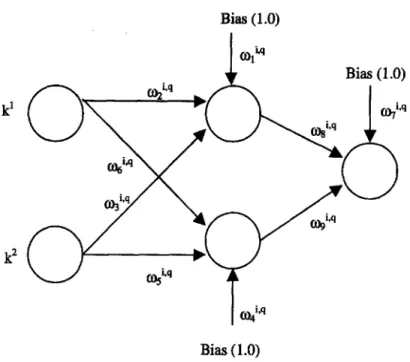
As for the neural net architectures, after a round of experimentations, we adopt a fully con- nected feedforward network from N& to parameterize the feedback production rule, q’(k,‘, k,“): as

qi (k,l&) = $v (&W”‘~) 1 ₍₁₈₎

for each player i = 1,2 (see Figure 1). The input vector to the networks at time t is V: = (Ici, lc:). In the hidden layer, the activation functions are linear. At the output level, the squashing functions are as in equation (9) except that we also let GAS search emin and emax rather than fixing them ahead.

Feedback investment policies, ZZ? (Icj , lci), on the other hand, are represented by a disconnected feedforward neural network from N$,4,1 (see Figure 2) as

’

The input vector to the networks at time t is rt = (ki, ki, Icz, $). We use sigmoid activation functions at both the hidden and the output layers.

Two GAS are then assigned to player i: GAi>q trains the neural net parameterizing the feedback production rule, @($; wz,Q), and GA”*” evolves the neural net parameterizing the feedback

(10)

Bias (1.0)

Bias ( 1 .O)

Figure 1. Neural network architecture for production policy rule.

Bias (1.0)

Figure 2. Neural network architecture for investment policy rule.

investment rule, c~~(T~;w~~~). To obtain k~,, (thus the input vectors at time t + l), we use

equation (19) in the state transition equation (16) for each player i as

ki

t+1 =cp i ($, Wi,r )+(1-E)kf, (20)

(11)

function to be maximized subject to equation (20), fl > 0 and ‘pi 2 0 becomes

T-l

jt (w1,q,“2,q,w1,~,w21~) = c 6t [pi ($5’ (z&w’+q ,qb2 (&w2q) 8 (q?2,q)

t=o (21)

-ci (I&

qY

(&Wi~“))

- h1

($2

($,Wi’“))]

In any generation, the duopoly game is repeatedly played starting from the given set of initial states:

fi = {(2,2)

,

(2,6)

,

(2312)

,

(62)

,

(6, f-3, (612)

>

(12: 2)

,

(1% 6)

,

(1% 12))

For any given set of weights and the initial states, (k:, ki) E II, the sample paths for the states, production and investment feedback policies are generated from the above maximiza- tion as {ki}T=&‘, (&($,~@)}~&i, and {@(r~,~~~~)}~&i, respectively. Thus, GAS search the weights of production and investment networks to maximize the sum of the payoffs over all initial states

subject to equation (20), & 2 0 and (p2 > 0.6

For each initial condition, the game is assumed to become stationary after 100 periods and the stationary tails are appended to the truncated objective functionals as in [2].

In every generation s E S, GAi>j (i = 1,2; j = q,z) operates on a constant size population. N2,3, of neural net weights

Pop”d (s) = {“:.j (s) ,w;j (s) ). , w?j (s) (. ) w;!,, (s)} ,

where W:“(S) E Popij(s) is the weights of a potential neural network, that approximates the

player i’s optimal production policy for j = q and optimal investment policy for j = z. GA114 evaluates each individual b E PoP”~(s) by computing its raw fitness

3 ( w;*q

(s)

) wl,s*

(s - 1) ,&q* (s _ 1)

) W2,r*

(s - 1,)

T-l

= c c bt [d (4’ (&w;‘q(s)) d2 ($,w2,q* (s - 1,)) $1 (v;,w;,q (s))

(k;,k;)ErI t=o

-cl (k:; I$ (vt”,wp (s))) - h’ ((2 (L& wl,s* (s - l)))] ,

where w’~~*(s - l), w2v’J*(s- l), and w2jr*(s - 1) are the previous best weights in the populations

of GAIJ GA2,q and GA2J, respectively.

Similaily, other GAS, GA1+, GA2yg, and GA’>“, compute the raw fitnesses, ?(wl@(s ~

1),w~~x(s),w2~q*(s - q,w2+* (s - 1)) for all d E Pop”“(s), j2(w1@(s - ~),w~,~*(s - 1):

wp(s), w2J’ (f - 1)) for all e E POPISH, and j2(w1+J*(s - l), wlJ*(s - l), w2,‘J*(s - l), w;‘~(s)) for ail f E Pop215(s), respectively.

The search starts with random populations, Pop’>*(O), Pop’>‘(O), PoP~>~(O), and Pop2~“(0). In our simulations, the interconnection weights for investment and production neural nets are searched in the interval [-5,5], with the exception of Bmin and emax for which the search intervals are emin E [O, 31 and 8,, E [O, 151.

6When a string representing the weights of a network violates the control bounds, it is punished by a high penalty; namely - 1000000 * Icf * kf

(12)

The genetic operators were done using the public domain Genesis 5.0 package [20] in parallel. We compile Genesis 5.0 on a SUN SPAC-1000 running Solaris 2.5. We run the experiment 50 times. In every run, we use population sizes of 50, crossover rates of 0.60, and mutation rates of 0.001 for each GA.

4.1. Results

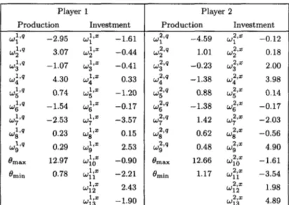
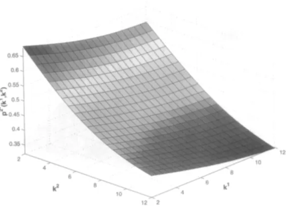
The best weights for the policy functions over all runs are reported in Table 1. Figures 3-6 depict the best policy functions. Note that, even though Players 1 and 2 are symmetric and should have the same feedback policies, neural network specification and GA training result in slightly different policies. Thus, we report the best weights and graphs of the policy functions for both players.

Table 1. The best weights for the feedback policy functions.

Player 1 Player 2

Production Investment Production Investment

Wl 162 -2.95 w;+ -1.61 w1 219 -4.59 wy -0.12 w2 14 3.07 w;+ -0.44 w;,q 1.01 w;+ 0.18 w3 14 -1.07 wp -0.41 wp -0.23 ~32,~ 2.00 w4 IA 4.30 wp 0.33 wy -1.38 w;‘~ 3.98 w5 l,q 0.74 wp -1.20 w5 239 0.88 wp 0.14 w6 14 -1.54 wp -0.17 wp -1.38 ~62’~ -0.17 l,q w7 -2.53 w;‘= -3.57 w;+J 1.42 w;,, -2.03 WE 14 0.23 w;,= 0.15 wp 0.62 w;+ -0.56 l,rl w9 0.29 wp 2.53 w;‘~ 0.48 w;‘= 4.90

I3 nlax 12.97 _WlOl+ -0.90 emax 12.66 WlO 2,s -1.61

emin 0.78 Wiiz -2.21 emin 1.17 Wfiz -3.54

w12 17 2.43 w12 2,x 1.98 w13 181 -1.90 w13 2,s 4.89 0.65 0.6 -0.55

%

-x^ 0.5

.-

ho.45 0.4 0.35 2

(13)

Genetic Neural Networks 0.65 0.6 -0.55 "x -i 0.5 s- "p. 0.45 0.4 0.35 2 12 12 2

Figure 4. Player 2’s equilibrium price, pz* (kl , k2)

10, 6- 7- e 54 6- ', = 5- 4. 3. It: >

(14)

1506 S. SIR~KAYA AND N. M. ALEMDAR

. -12

Figure 6. Player 2’s equilibrium production levels, q2* (Icl, /c’).

Observe from Figures 3-6 that with an increase in players’ own capital stocks, production costs diminish. Hence, equilibrium prices drop, while equilibrium quantities increase in player’s own capital stock. An increase in the rival’s capital stock, on the other hand, makes the rival more cost effective, and decreasing, therefore, both the equilibrium price and the equilibrium production levels of both players.

-12

(15)

Genetic Neural Networks

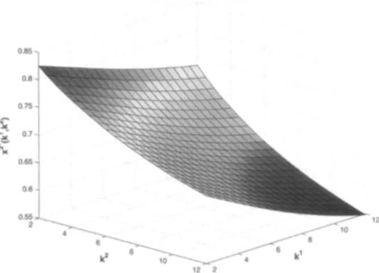
Figure 8. Optimal investment for Player 2, x2’(k’, !I?).

Figures 7 and 8 show the optimal investment strategies as smooth decreasing functions of both capital stocks. When player’s own capital stock is lower than the steady state, the optimal strategy is to invest as much as possible also paying heed to the fact that too fast an adjustment is costly. If, however, the initial capital stock is large relative to the steady state, it is optimal to allow the capital to depreciate down to the steady-state level. The steady state is determined by the conditions z”(lcl, k2) = E/?, i = 1,2, that is, optimal investments are just sufficient to replace the worn out capital in the steady state.

4.2. Robustness

To test how good the trained networks generalize, the following initial states are chosen:

li = {(1.5,1.5),(1.5,3.5), (1.5,6.5), (1.5,12.5), (3.5,1.5),(3.5,3.5), (3.5,6.5), (3.5,12.5), (6.5,1.5), (6.5,3.5),(6.5,6.5),(6.5,12.5),(12.5,1.5),(12.5,3.5), (12.5,6.5), (12.5,12.5)}

Note that to measure the out of sample performance of the trained neural nets, the initial states in I? are different from the ones in II.

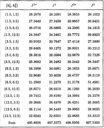
We measure the performance of our approximation by the following statistic:

c

J” (k&k;) -

c

Jz* (k&k:)

Opt2 = (k&kf)Eli (k;,k;)Efi

C J” (k& k,2) ’

where J”* is the payoff of player i using the stationary equilibrium policies using the weights in

Table 1. Jis, on the other hand, are computed in from each pair initial states given in fi for each player by retraining the neural nets 50 times. We report the best performance over all runs.

The values of Ji and Ji* are shown in Table 2. Note again that, as neural network specification and GA training result in slightly different policies even though the players are symmetric, we report Js and J*s for both players. From Table 2, the calculated Opt’ is 0.0029 and Opt? is 0.0017, which verifies that the trained networks are indeed robust.

(16)

Table 2. Out of sample performance.

J” J’ J2’ 52 (1.5,1.5) 28.2976 28.2391 28.3655 29.1052 (1.5,3.5) 27.3449 27.3456 30.9857 30.9451 (1.5,6.5) 26.0716 26.0865 34.2395 34.1915 (1.5,12.5) 24.3447 24.3481 39.7772 39.8923 . (3.5,1.5) 30.9162 30.7647 27.4118 27.3890 (3.5,3.5) 29.8405 30.1272 29.9021 30.2212 (3.5,6.5) 28.3816 28.3994 32.9879 32.7326 (3.5,12.5) 26.3682 26.2482 38.2442 38.3447 (6.5,1.5) 34.1958 34.6961 26.1653 25.8671 (6.5,3,5) 32.9640 33.4026 28.4737 28.3119 (6.5,6.5) 31.2560 31.2379 31.3178 31.4981 (6.5, 12.5) 28.8571 28.9319 36.1266 36.2030 (12.5,1.5) 39.7452 39.8180 24.3984 24.3276 (12.5,3.5) 39.2666 38.4976 26.4251 26.3665 (12.5,6.5) 36.1114 36.5443 28.9063 28.8035 (12.5,12.5) 32.9242 32.6501 32.9685 33.3310 Sum 495.8856 497.3373 496.6956 497.5303

5. CONCLUSION

We have developed a new method to efficiently approximate the feedback Nash equilibria in dynamic games. In the algorithm, players’ feedback rules are represented by feedforward neural network architectures which are trained online synchronously by genetic algorithms in a parallel manner to search over all time-invariant equilibrium strategies.

Neural network specification offers important flexibility over the traditional techniques, such as spline functions or RBFs. There are several good reasons for our choice of genetic algorithms (GA) to train the neural networks as well. An important advantage in GA search is the fact that regardless of the initial parameter values, they ensure converge to an approximate global optimum by exploiting the domain space and relatively better solutions through genetic operators. Another feature of GAS which we exploit in our game algorithm is their explicit parallelism.

In the algorithm, each feedback rule is parameterized by the weights of a suitable neural network, thereby transforming the players’ strategy spaces from sets of rules to sets of neural net weights. For each network, an artificially intelligent player, a GA, is assigned to breed fitter weights and update other GAS via the computer shared memory as to its best-to-date feedback rule. In any given generation, the game starts from multiple sets of initial states. As we search for the stationary feedback rules, the same set of neural net weights are employed to compute

the overall payoffs as the raw fitness. Our rationale for repeating the game is two-fold:

to avoid the dependence of the weight training on the initial conditions and also to speed up GA learning.

Essentially, each GA trains a neural network online to best respond to the other players’ best feedback rule in the previous generation. The fittest weights are then communicated to each other via the computer shared memory. Equipped with the updated weights, each player is better able to anticipate the best response of the others for all potential rules in its population. The individuals which exploit this knowledge to their advantage are fitter, thus reproducing faster.

(17)

Ultimately, the fitter weights dominate the respective populations also steering the other players‘ search for the best set of rules to the vicinity of the feedback Nash equilibrium.

REFERENCES

I, M.J. Miranda and D.V. Vedenov, Numerical solution of dynamic oligopoly games with capital investment, Economic Theory 18, 237-261, (2001).

2. N.M. Alemdar and S. bzydchnm, A genetic game of trade, growth and externalities, Journal of Econom?c, Dynamics and Control 22, 81 l-832, (1998).

3. S. Clemhout and H.Y. Wan, Jr., A class of trilinear differential games, Journal of Optimizatzon Theory and Applications 14, 419-424, (1974).

4. E.J. Dockner, G. Feichtinger and S. Jorgensen, Tractable classes of nonzero-sum open-loop Nash differential games: Theory and examples, Journal of Optimization Theory and Applications 45, 179-197, (1985), 5. C. Fershtman, Identification of classes of differential games for which the open-loop is a degenerated feedback

Nash equilibrium, Journal of Optimization Theory and Applications 55, 217-231, (1987).

6. A. Mehlmann and R. Willing, On nonunique closed-loop Nash equilibria for a class of differential games with a unique and degenerate feedback solution, Journal of Optimization Theory and Applications 41, 463-472. (1983).

7. J. Reinganum, A class of differential games for which the closed loop and open loop Nash equilibria coincide. Journal of Optimization Theory and Applications 36, 253-262, (1982).

8. T. Bqar and G.J. Oldser, Dynamic Noncooperative Game Theory, Academic Press, New York, NY, (1982) 9. K. Funahashi, On the approximate realization of continuous mapping by neural networks, Neural Netzuorhs

2, 183-192, (1988).

10. K. Hornik, M.H. Stinchcombe and H. White, Multilayer feedforward networks are universal approximators. Neural Networks 2, 359-366, (1989).

11. K.S. Narenda and K. Parthasarthy, Identification and control of dynamical systems using neural networks. IEEE Rznsaction on Neural Networks 1 (l), 4-27, (1990).

12. FL. Hecht-Nielsen, Neurocomputing, Addison-Wesley, Massachusetts, (1990).

13. J. Hertz, A. Krogh and A.G. Palmer, Introduction to the Theory of Neural Computation, Addison-Wesley. Massachusetts, (1991).

14. J.H. Holland, Adaptation in Natural and Artificial Systems, The University of Michigan Press, Ann Arbor. MI, (1975).

15. H. Miihlenbein, Darwin’s continent cycle theory and its simulation by the prisoner’s dilemma, In Toward a Practice of Autonomous Systems: Proceedings of the First European Conference on Art@ial Life, (Edited by F. J. Verela and P. Bourgine), pp. 236-244, (1992).

16. S. Ozylldlnm, Three-country trade relations: A discrete dynamic game approach, Computers Math. Applrc 32 (5), 43-56, (1996).

17. N.M. Alemdar and S. Sirakaya, On-line computation of Stackelberg equilibria with synchronous parallel genetic algorithms, Jozlrnal of Economic Dynamics and Control 27, 1503-1515, (2003).

18. J. Branke, Evolutionary algorithms for neural network design and training, Technical Report, NO. 322. University of Karlsruhe, Institute AIFB, (1995).

19. K. Judd, Cournot vs. Bertrand: A dynamic resolution, Working paper, Stanford University, (1996). 20. J.J. Grefenstette, A user’s guide to GENESIS version 5.0, Manuscript, (1990).

21. J. Mercenier and P. Michel, Discrete-time finite horizon approximation of infinite horizon optimization prob. lems with steady-state invariance, Econometrica 62, 635-656, (1994).