Bluetooth or 802.15.4 Technologies to Optimise
Lifetime of Wireless Sensor Networks: Numerical
Comparison Under a Common Framework
Chiara Buratti
†, Ibrahim Korpeoglu
‡, Ezhan Karasan
‡, Roberto Verdone
††
CNIT, IEIIT-BO/CNR, DEIS, University of Bologna, Bologna, Italy
Email: [email protected], [email protected]
‡
Depts. of CE and EE, Bilkent University, Ankara, Turkey
Email: [email protected], [email protected]
Abstract— This paper aims at comparing through simulations
the network lifetime of a wireless sensor network using Bluetooth-enabled or IEEE802.15.4 compliant devices. The evaluation is performed under a common reference framework, namely the EMORANS scenario for wireless sensor networks. Since the two enabling technologies rely on different MAC paradigms, suitable definition of the performance metrics is needed, in order to make the comparison meaningful. Thus, the paper has also a methodological objective. In particular, three different definitions of network lifetime are introduced, and a comparison of performance obtained by applying the different definitions is provided. Then, the comparison between the two standards is introduced: it is shown that there are no orders of magnitude of difference in network lifetime when the two technologies are used and the choice of the technology depends on the application requirements.
I. INTRODUCTION
IEEE 802.15.1 (Bluetooth) [1] and IEEE 802.15.4 [2] are two short-range, low-power, low-cost wireless communica-tion technologies that enable formacommunica-tion of wireless networks among devices, computers, consumer electronics equipments, sensors and actuators. The type of network applications where these technologies can be used include Wireless Sensor Net-work (WSN) applications. WSNs are built from nodes that have to be low cost and that should require very low power consumption. These two requirements can be satisfied with these technologies. These two technologies, however, differ in a lot of aspects. Depending on the application type, the envi-ronment, the sensor node technology, and the network config-uration requirements, we believe that there will be cases where 802.15.4/Zigbee will be preferred over 802.15.1/Blueooth, and there will be cases where the opposite is true. Therefore there is clear need to analyze Bluetooth and IEEE 802.15.4 with respect to each other in order to be able to decide which technology would be more suitable for a given application with certain constraints and requirements.
In this paper we numerically address the issue of network lifetime, being one of the most important for WSNs. The goal is to compare these two technologies with each other in
This work is done as part of NEWCOM (Project No: 507325) and NEWCOM++ (Project No: 216715) Projects (Network of Excellence in Wireless Communications) funded by Europian Commussion through FP6 and FP7 framework programs.
terms of network lifetime considering an application typical of WSNs, namely, environmental monitoring, where a sink periodically needs to collect the measurements performed over the sensed area by nodes. We denote as round the time elapsing between two successive measurements.
There are some studies that compare Bluetooth and IEEE 802.15.4 [3]. There are also studies that compare Bluetooth to IEEE 802.11 [4]. These works, however, are not done in the context of WSNs. As far as we know, this is the first study that compares these technologies in the context of WSNs.
Since Bluetooth uses a collision free MAC protocol, while 802.15.4 merges contention based (i.e. Carrier Sensing Multi-ple Access with Collision Avoidance, CSMA/CA) and con-tention free strategies, the QoS requirements of the two networks in terms of the amount of information that the sink has to receive at each round, have to be defined properly to build a meaningful comparison. This aspect is addressed in the Section reporting the numerical results, where three different definitions of network lifetime are introduced and a comparison of performance obtained by using these definitions is performed.
The rest of the paper is organized as follows. Next Section will introduce the reference scenario used in the paper. Sec-tion III provides details about the protocols implemented in the two simulators. Section IV provides and discusses numerical results; and the last Section reports a summary of the main achievements.
II. EMORANS SCENARIO
EMORANS is an integration activity developed in NEW-COM (the Network of Excellence in Wireless Communica-tions funded by EC-IST through FP6) [5]; it is actually an extension of an initiative that started in COST273 some years ago. It aims at the definition of reference scenarios for the evaluation of wireless networks, with the objective of making more comparable the results achieved by different research groups, which use different evaluation tools.
Very recently, an EMORANS reference scenario for WSNs has been developed [6]. This is the first paper using it.
EMORANS for WSNs provides the description of the network geometrical layout, the physical layer aspects, the
energy consumption model, etc. Once the objective of a given evaluation is fixed, one has to pick from the EMORANS elements (i.e. the entities describing a model, or providing the realisations, etc.) those who are not subject to optimisation. The latter are the objective of the study, and are left to the will of the researcher. EMORANS also provides the definition of some performance figures. Once the majority of inputs to the evaluation tools are common, it is much more meaningful to compare results achieved by different tools/groups.
The EMORANS elements taken for this paper are as fol-lows:
• geometrical layout: a square of side set to 100 m; • the node density: either 100 or 500 nodes are considered,
with uniform distribution over the square;
• the sink is located in the centre of the square;
• the initial battery charge, set at 1 Joule to have shorter
simulations;
• channel model: loss in logarithmic scale isk0+k1ln d+s
where d is distance and k0= 40 dB, k1= 13.03 (these
values are obtained through experimental measures made on the field in a rural environment) and s is a Gaussian
random variable, having zero mean and standard devia-tionσ, modelling channel fluctuations; the capture packet
model used states that a packet is correctly received in case the loss is smaller than a given threshold,Lm, which
depends on the technology used;
• the definition of network lifetime (see Section IV).
Concerning all other parameter values, they have been set according to the objective of this paper: comparison be-tween Bluetooth and 802.15.4. The energy consumption model reflects choices that are specific of commercially available devices for the IEEE802.15.4 technologies; whereas for Blue-tooth the values of the energy spent to transmit and receive a bit are taken to be similar to the ones in [7]. These values will be reported in the following Section.
III. SIMULATIONMODELS ANDALGORITHMS
We simulated Bluetooth and IEEE802.15.4 protocols to evaluate performance in terms of network lifetime using these technologies. Starting from the EMORANS scenario (see Sec. II), we have developed two different simulators (written in C++ language) for the two technologies, to obtain comparable results. The physical and MAC layer protocols are compliant with the two standards [1], [2]; where as the routing protocol an N -level tree-based topology is considered in both cases.
But, being the number of nodes (slaves) per parent (master) limited in Bluetooth, the tree developed in the Bluetooth simulator has no height limits (N is unlimited), whereas a
limit (equal to seven) is imposed on the number of children per parent. On the other side, since the IEEE802.15.4 standard does not impose a limit on the number of children per parent, in this simulator we consider a three-level topology with an un-limited number of children per parent. In the following, more details about the protocols developed in the two simulators will be given.
A. Bluetooth
The Bluetooth technology is simulated as follows. At the beginning of each simulation, a Bluetooth scatternet is formed according to the Bluetrees scatternet formation algorithm avail-able in the literature [8]. In this algorithm, the sink node is the root of the tree and the sensor nodes constitute the intermediate and leaf nodes of the tree. Master, slave and bridge roles are then assigned to the Bluetooth capable sensor nodes. Leaf nodes are slaves, the root is a master, and the intermediate nodes are bridges of type master/slave (M/S). This means, an intermediate node is a master of its children nodes, but is a slave of its parent node in the tree. While forming the tree, Bluetrees algorithm ensures that there will be at most 7 slaves connected to a master in a piconet.
After the scatternet is formed, the data gathering process from the square region is simulated. The gathering process happens in rounds, and in each round all sensor nodes are able to send their sensed data to the sink. There is no aggregation applied, hence there will be a different packet arriving to the sink from each sensor node.
The data gathering process at each round is triggered by the sink by broadcasting a control packet (i.e. a query packet) throughout the scatternet. The size of the control packet payload is assumed to be 10 bytes. Each node will receive this packet, sense the environment, obtain the data, and will finally send it towards the sink using possibly one or more sensor nodes in between. The size of the data packet payload is assumed to be 16 bytes. In Bluetooth, a payload of that size can be carried within a DM1 or DH1 baseband layer packet [1]. We assume DH1 packets are used, where no FEC encoding is applied to protect the payloads. The payload header for a DH1 packet is 1 byte, and there is a 2 bytes of CRC added to the end of the payload. The Bluetooth baseband layer overhead that is added before the payload header is 16 bytes (72 bits for access code, 54 bits for 1/3 FEC coded baseband header); therefore, the total size of a data packet is assumed to be 35 bytes (16 + 1+ 16 + 2), and the total size of a control packet is assumed to be 29 bytes. Additionally, for every data packet transmitted from a slave to a master, the master has to poll the slave first, and therefore we also need to consider the POLL packets of Bluetooth basedband layer as part of the communication overhead causing energy consumption. A POLL packet does not carry a payload information, therefore does not have a payload header nor a CRC. Hence, we take the size of a POLL packet as 16 bytes (72 bits access code and 54 bits header).
For multiplexing of traffic, Bluetooth uses a polling-based TDMA MAC protocol inside a piconet, and an FHSS based spread spectrum scheme among piconets. Hence, there can be overlapping piconets without interferring with each other. Inside a piconet, the polling based MAC protocol ensures that there are no packet collisions. It operates as follow. Time is slotted, and a Bluetooth DM1, DH1, or POLL packet can fit into a single time slot. Half of the time slots (even-numbered slots) are used for master-to-slaves communication, and the other half (odd-numbered slots) are used for slaves-to-master communication. In a Round-Robin fashion, the master can
directly send data packets to slaves using the even numbered time slots. Similarly, in a Round-Robin fashion and using the even-numbered time slots, the master can poll the slaves so that the slaves can send data to the master in the subsequent odd-numbered time slots. When the master polls a slave by sending a POLL packet, the slave can respond with a data packet in the next time slot, if it has some data waiting to be sent to the master. In the next even-numbered time slot the master can poll another slave or can send data to another slave. The Bluetooth MAC protocol does not allow slaves to talk to each other directly; all traffic has to go through the master node.
We assume a Bluetooth transceiver consumes 0.1
µJoule/bit, to transmit and receive a bit [7] and nothing if it
is not sending or receiving anything (sleep mode). We ignore the energy spent for outputting the packet at the antenna, since the Bluetooth range is very short and very low output power (around 1 mW) is used. To compute the energy per packet transmission (or reception), we multiply the energy spent to transmit (or receive) a bit with the packet size (in bits). The transmit power used by nodes and by the sink is set to 0 dBm and the receiver sensitivity is -70 dBm (i.e.,
Lm= 70 dB). B. IEEE802.15.4
The three-level tree based topology, composed of the sink (level zero), a number of Cluster Heads (CHs) connected to the sink (level one) and non-Cluster Heads (level two) transmitting to the sink through a two-hop communication, is developed according to the following steps. A certain number of nodes in the network elect themselves CHs, through a distributed self-election algorithm: nodes elect themselves CHs with probability px. Each CH broadcasts a packet informing of its role and those nodes that did not elect themselves as CHs (non-CHs) select their CH to transmit to, on the basis of the power received by each CH. In particular, each node selects the loudest CH, that is the one from which it receives the largest power. Once the tree is formed, a number, Ntr,
of rounds follow, devoted to the sample transmissions by the nodes. At every round each non-CH node transmits its sample in a short packet to the respective CH, which, on its turn, sends all samples received, plus the one it generated, to the sink via a direct link, putting together the various samples in a single packet. The choice of Ntr should represent a compromise
between the desire to keep a low overhead, requiring Ntr
large to amortize the time and energy spent for the topology formation phase, and the need to rotate often the role of CHs among nodes, since being a CH is much more energy consuming than being a non-CH [9].
As far as MAC layer, the slotted CSMA/CA protocol developed in the simulator is the standard IEEE 802.15.4 slotted CSMA/CA protocol [2] with no battery life extension,
BEmin=3, BEmax=5 and N Bmax=4; for the sake of
con-ciseness we do not report its description here, but we refer to the standard. Here we only remind that N Bmax represents
the maximum number of times a node can try to access the channel for the transmission of the same packet. The
superframe structure is used as follows: non-CH nodes use the Contention Access Period (CAP) portion, in which the access is managed by CSMA/CA. Collisions inside the clusters may occur, whereas collisions between different clusters are avoided by associating different radio channels to the CHs and thus to the clusters (this allocation is provided by the sink during the transmission of the Beacon packet). CH nodes, instead, use the Guaranteed Time Slots (GTS), allocated by the sink during the Beacon transmission; till the number of CHs is smaller than seven (that is the maximum number of GTSs that could be allocated), collisions may not occur. When, instead, the number of CHs is larger than seven, they have to use the CAP to access the channel and collisions between CHs may occur.
The physical layer protocol is IEEE802.15.4 compliant: frequency, bit rate, and modulation are the same reported in the standard [2]; the packet sizes are standard compliant and are the following: the Beacon packet has a payload of 10 bytes and a total size of 62 bytes; the data packet has a payload of 16 bytes and a total size of 25 bytes and finally the acknowledge packet has a size of 5 bytes. Note that the payload size values are the same used for Bluetooth, to realise a coherent comparison. The values of the energy spent were obtained by the data sheets of the IEEE802.15.4 devices produced by Freescale; in particular each node spends 0.39
µJ/bit to receive and sense a bit and 0.32 µJ/bit to transmit
a bit. The energy consumption model is the same used in the Bluetooth simulator. The transmit power used by nodes and by the sink is set to 0 dBm and the receiver sensitivity is -92 dBm (i.e.,Lm= 92 dB).
IV. RESULTS ANDDISCUSSION
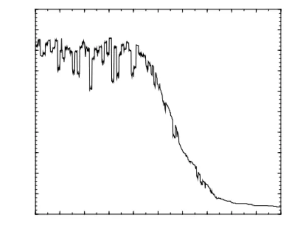
Performance is evaluated in terms of network lifetime. The following different definitions of network lifetime are given in the E-MORANS scenario: the interval of time (measured in rounds), started with the first transmission in the wireless network, ending when the percentage of nodes that have not terminated their residual energy (Def. 1), or the percentage of nodes that are still reachable in the network averaged over a time window (Def. 2), or the percentage of reports from nodes to the sink averaged over a time window (Def. 3), falls below a specific threshold, which is set according to the type of application (it can be either 100% or less). The first definition takes into consideration only energy consumption issues, whereas, the second considers both energy consumption and connectivity issues and, finally, the third refers to energy consumption, connectivity and MAC failures. The reason why we have to average results over a time window (Def. 2 and Def. 3) is the following: if we consider the number of packets received by the sink in the IEEE802.15.4 network as a function of the number of rounds (see Figure 1, obtained for a network of 500 nodes and settingσ = 0, Ntr= 10 and px = 0.03), we
obtain a non-monotone curve, which presents a lot of peaks. Thus, from this curve it is not easy to extract the network lifetime values for the different percentages and also to do a comparison with Bluetooth. To obtain a monotone curve, we average the number of packets received by the sink over 50
rounds (the time window) and we put this value over all the 50 rounds.
In Bluetooth, being collision free, MAC failures do not occur, thus Def. 2 and 3 coincide: a packet is lost when a node dies or when it cannot reach the final sink, owing to connectivity problems. For example, when a master dies, all its slaves, even if they are still alive, cannot reach the sink and their packets are lost. By comparing the results obtained from applying the two definitions (1 and 3) to a network composed of 500 nodes (we do not report here the figure, for the sake of conciseness), we obtain that when the number of reports arriving to the final sink (Def. 3) reaches zero, the number of nodes still alive is 493. When a node, in fact, can no longer reach the final sink, it will not transmit packets and thus it will not consume energy for the rest of the time. Thus, the number of nodes alive is still large when there are no more packets reaching the sink.
In the IEEE802.15.4 simulator, instead, packet losses are caused by the following events: a node is isolated, that is it does not receive the Beacon packet; a node does not succeed in transmitting correctly its packet by the end of the superframe portion devoted to this, and, finally, a packet is lost when a node does not succeed in accessing the channel for more than
N Bmax consecutive times, for the transmission of the same
packet.
In Figure 2, a comparison of results obtained by applying the three different definitions at the IEEE802.15.4 simulator, is provided. We have considered a network composed of 500 nodes and we have set σ = 3.5, Ntr = 10 and px = 0.03. In
this case the time window has been set to 200. As we can see the three curves are quite different, thus a proper definition of the metric is fundamental to do coherent comparisons of results.
In Figure 3, a comparison between Bluetooth and IEEE802.15.4 is provided, by considering two networks com-posed of 500 (in this case for IEEE802.15.4 we setNtr= 10
andpx = 0.03) and 100 nodes (in this case for IEEE802.15.4
we set Ntr = 10 and px = 0.15). The Figure shows the
number of rounds in which reports from a certain percentage of nodes are still arriving to the sink (Def. 3), by varying the percentage. In other words, the Figure shows the rounds at which the number of reports still arriving to the sink from nodes starts falling below a certain percentage (a threshold) which is denoted at the x-axis. Note that, we do not show
results relative to 90% and 100% in the 100 nodes case and to 80%, 90% and 100% in the 500 nodes case, for the IEEE802.15.4 simulator, because already in the first round more than the 10% of packets in the 100 nodes case, and more than the 20% of packets in the 500 nodes case, are lost. As we can see, IEEE802.15.4 performance results are better than the ones obtained with Bluetooth, if we consider the cases in which IEEE802.15.4 performance results are shown. Thus, we can deduce that the choice of the technology depends on the application requirement; if, in fact, we consider a network composed of 100 nodes, and an application which impose the sink receives the 100% or the 90% of the packets, we have to choose Bluetooth, because the IEEE802.15.4 cannot reach these percentages. In case, instead, the application can tolerate
that more than the 10% of packets are lost, IEEE802.15.4 works better, because it realises a more energy efficient network. Thus, the choice of the technology depends on the application requirement.
V. CONCLUSIONS
The paper compares network lifetime of a wireless sensor network using Bluetooth-enabled or IEEE802.15.4 compliant devices, through simulations. A common reference framework (EMORANS scenario) is considered to make a coherent comparison. After the introduction on three different network lifetime definitions and the comparison of results obtained by applying these definitions, a comparison of IEEE802.15.4 and Bluetooth performance is provided. It is shown that the choice of the technology depends on the application requirement. In particular, in case the application can tolerate some losses of packets, IEEE802.15.4 performance results are better than the ones obtained with Bluetooth, although there are no orders of magnitude of difference; whereas, in case the application re-quires that a large number of reports reach the sink, Bluetooth must be chosen.
REFERENCES
[1] IEEE 802.15.1: Wireless Medium Access Control (MAC) and Physical Layer (PHY) Specifications for Wireless Personal Area Networks (WPANs), IEEE, 2002. URL: http://standards.ieee.org/getieee802/802.15.html
[2] IEEE 802.15.4: Wireless Medium Access Control (MAC) and Physical Layer (PHY) Specifications for Low-Rate Wireless Personal Area Net-works (LR-WPANs), IEEE, 2003.
[3] “Zigbee and Bluetooth: Strength and Weaknesses for Industrial Applica-tions”, IEE Computing and Control Engineering, April/May 2005. [4] E. Ferro, F. Potorti, “Bluetooth and Wi-Fi Wireless Protocols: A Survey
and Comparison”, IEEE Wireless Communications, February, 2005. [5] NEWCOM - Network of Excellence on Wireless
Com-munications, Europian Commission IST FP6 Project, ”https://newcom.ismb.it/public/index.jsp”.
[6] C. Buratti, “Second report on common frameworks/models matching Project A needs”, Sixth Deliverable of Project A of NEWCOM, February 28, 2006.
[7] O. Kasten, M. Langheinrich, “First Experiences with Bluetooth in the Smart-Its Distributed Sensor Network”, Proceedings of Workshop on Ubiquitous Computing and Communications, Barcelona.
[8] G. V. Zaruba, S. Basagni, and I. Chlamtac, “Bluetrees-scatternet forma-tion to enable bluetooth-based ad hoc networks”, Proceedings of IEEE International Conference on Communications, volume 1, pages 273– 277, June 2001.
[9] C. Buratti, R. Verdone, “On the Number of Cluster Heads Minimizing the Error Rate for a Wireless Sensor Network Using a Hierarchical Topology over IEEE802.15.4”, IEEE PIMRC2006, Helsinki, FL, Sept 11-14, 2006.
0 100 200 300 400 500 600 700 800 900 1000 Number of Rounds 0 50 100 150 200 250 300 350 400 450 500
Number of pakets received by the sink
Fig. 1. Number of packets received by the sink as a function of the number of rounds, for the IEEE802.15.4 network.
0 200 400 600 800 1000 1200 1400 1600 1800 Number of rounds 0 50 100 150 200 250 300 350 400 450 500 550
Number of nodes still alive Number of nodes still reachable Number of reports to the sink
Fig. 2. Comparison of the different network lifetime definitions for the IEEE802.15.4 network.
40 50 60 70 80 90 100 110 0 500 1000 1500 Network Lifetime Bluettoth 100 nodes IEEE802.15.4 100 nodes Bluetooth 500 nodes IEEE802.15.4 500 nodes
Fig. 3. Network Lifetime comparison between Bluetooth and Zigbee, for a network composed of 100 and 500 nodes. The x-axis denotes the threshold value (x%).