A s. J o>f -'’' 1.. S \, aLVj_i ' . . ‘ V % J i J - ·*·*4 V/*' ,>■’·■; ■•■Víi'^ '· S..·. # f:,5£ ií
R IP P L E -F R E E D E A D B E A T C O N T R O L
OF S A M P L E D -D A T A S Y S T E M S
A THESIS
SUBMITTED TO THE DEPARTMENT OF ELECTRICAL AND ELECTRONICS En g in e e r in g
AND t h e i n s t i t u t e OF ENGINEERING AND SCIENCES OF BILKENT UNIVERSITY
IN PARTIAL FULFILLMENT OF THE REQUIREMENTS FOR THE DEGREE OF
MASTER OF SCIENCE
Erkan Ünal Mıımcuoğlu M ay 1990
© Copyright May, 1990 by
Erkan Ünal Mumcuoğlu
Ь . 2 2 8 3
Q V í Ц 0 2 . • Ь Ѵ %
I certify that I have read this thesis and that, in my opinion, it is fully adequate, in scope and in quality, as a thesis for the degree of Master of Science.
Prof. Dr. M. Erol Sezer (Principal Advisor)
I certify that I have read this thesis and that, in my opinion, it is fully adequate, in scope and in quality, as a thesis for the degree of Master of Science.
Assoc. Prof. A. Bülent Özgüler
I certify that I have read this thesis and that, in my opinion, it is fully adequate, in scope and in quality, as a thesis for the degree of Master of Science.
Approved for the Institute of Engineering and Sciences:
Prof. Dr. Melimet Baray
Director of Institude of Engineering and Sciences
A B S T R A C T
RIPPLE-FREE DEADBEAT CONTROL PROBLEM
Erkan Ünal Mumcuoğlu M.S. in Electrical and Electronics Engineering Supervisor: Prof. Dr. M. Erol Sezer
February, 1990
In this thesis, we consider the ripple-free deadbeat control problem for linear, multivari able sampled-data systems represented by state-space models. Existing results concern ing the deadbeat/ripple-free deadbeat regulation and tracking problems are based on controller configurations of either constant state-feedback or discrete dynamic output feedback. In the thesis, the problem is analyzed for two new sampled-data controllers, namely, generalized sampled-data hold functions and multirate-output controllers. Some necessary and sufficient solvability conditions for the problem are stated by theorems in time-domain and frequency domain in terms of the open-loop system parameters. Sev eral special cases are also considered as corollaries.
Key words: Multivariable Systems, Sampled-Data Systems, Ripple-Free Deadbeat Control, Tracking, Regulation, Generalized Sampled-Data Hold Functions, Multirate- Output Controllers.
ÖZET
DALGACIKSIZ SIFIRA DÖNÜMLÜ DENETİM KURALI
Erkan Ünal Munacuoğlu
Elektrik ve Elektronik Mühendisliği Bölümü Yüksek Lisans Tez Yöneticisi: Profesör Dr. M. Erol Sezer
Mayıs, 1990
Bu tezde, durum uzayında tanımlanmış, doğrusal, çok değişkenli örneklenmiş sistem lerin dalgacıksız sıfıra dönümlü denetim problemi araştırılmıştır. Sıfıra dönümlü ve dalgacıksız sıfıra dönümlü izleme ve düzenleme amaçlı denetleyicilere ilişkin varolan sonuçlar sadece değişmez durum geribeslemeli ya da zamanda ayrık dinamik çıkıştan geribeslemeli denetim yapıları için elde edilmiştir. Bu tezde ise problem iki yeni bilgi örnekleme denetleyici sistemi kullanılarak analiz edilmiştir. Bu yöntemler, genelleştirilmiş bilgi örnekleme-tutma fonksiyonları ve farklı sıklıkta çıkış örnekleyici denetleyicilerdir. Teoremlerde verilen gerek ve yeter çözüm koşulları hem zaman hem de frekans tanım bölgelerinde açık döngü sistem değişmezleri türünden ifade edilmiştir. Özel durumlar ise teoremlerin sonuçlarında incelenmiştir.
Anahtar sözcükler: Çok Değişkenli Sistemler, Örnekleme-Tutma Sistemleri, Dal- gacıksız Sıfıra Dönümlü Denetim, İzleme Problemi, Durağanlaştırma problemi, Genelleş tirilmiş Bilgi Örnekleme-Tutma Fonksiyonları, Farklı Sıklıkta Çıkış Denetleyicileri.
A C K N O W L E D G E M E N T
I am grateful to Prof. Dr. M. Erol Sezer for his invaluable guidance, suggestions and helps during the development and writing of this thesis.
It is my pleasent duty to express my thanks to all individuals who assisted in the typing and gave suggestions. In particular, I would like to thank Assoc. Prof. A. Bülent Özgüler for his kindly helps and suggestions.
C on ten ts
1 INTRODUCTION
1
1.1 N o ta tio n ... 5
2 RIPPLE-FREE DEADBEAT CONTROL USING GSHF’s
6
2.1 Formulation of the P r o b le m ... C 2.2 Deadbeat Control Problem ... 102.2.1 General Solvability C o n d itio n ... 11
2.2.2 Implications of the Main T h e o r e m ... 13
2.2.3 Realizations of Generalized Sampled-Data Hold F u n c tio n s... 17
2.2.4 Geometric Solvability C o n d itio n s... 19
2.3 Ripple-Free Deadbeat Control Problem ... 22
2.3.1 General Solvability C o n d itio n s ...22
2.3.2 Ripple-Pree Deadbeat R egulation... 2G
3 RIPPLE-FREE DEADBEAT CONTROL USING MROC’s
28
3.1 Formulation of the P r o b le m ... 283.2 A Solvability C o n d itio n ... 33
3.3 Ripple-Free Deadbeat R eg u latio n ...37
4 CONCLUSIONS
39
REFERENCES
41
List o f F igures
2.1 Control Scheme with GSHF Controller
3.1 Control Scheme with Multirate-Outpiit Controller ... 29
C hapter 1
IN T R O D U C T IO N
Since World War II, the digital computers have experienced a period of remarkable growth, because their application to scientific computation provide high accuracy, com putational speed as well as flexibility and versatility. As advantages over analog tech niques became apparent, it seemed quite natural that control system engineers should also consider the application of digital techniques in control system design. By the use of sampling, a continuous-time system can be converted into a discrete-time system upon which digital control techniques can be applied easily to change both the continuous- and discrete-time behavior of the system in a desired way.
One of the fundamental problems associated with discrete-time control of linear (either discrete- or continuous-time) systems is that of driving some signals to zero in finite time and holding it there for all discrete ( sampling ) times thereafter. This problem is called the deadbeat control problem, since the signals are beaten to a dead stop.
If it is the system’s state which is to be driven to zero in finite time, then the problem is deadbeat state regulation [1],[2], and the very definition of controllability can be applied to solve this problem. The state deadbeat controller is independent of the system’s initial state and results in a nilpotent state transition matrix.
Deadbeat regulation problem arises if it is the system’s output that is to be driven to zero in finite time. This problem was solved by Leden [3] using state feedback, who pointed out that the closed-loop sometimes loses stability and the control input diverges exponentially to keep the output zero. In many applications, such a situation is not acceptable, therefore, controllers should be designed such that the control input converges to zero as time goes to infinity. Leden proposed in [3] a procedure for designing such a controller for a rather restricted class of systems.
Akashi & Imai [4] extended this result to the case of output feedback. They derived an elegant geometric characterization of the settling time, inspired by the geometric approach developed by Wonham [5]. Kimura & Tanaka [6] considered the problem with internal stability constraint in its full generality.
A more difficult problem is deadbeat tracking, when one wishes the output of the given system to track a reference signal in a deadbeat fashion. Such a deadbeat controller is a dynamic system which depends on the initial states of both the given plant and the reference generator. The earlier works of Tuo [7] and Kuçera [8] do not insist on the independence of the controller upon the initial states. The most complete results were given by Kuçera & Şebek [9], whose approach was in the transfer function setting, with dynamic output feedback configuration. They also showed that the same problem is solvable with internal stability constraint if and only if no unstable poles of the reference generator occur as a zero of the plant.
CHAPTER L INTRODUCTION 2
However, since ordinary deadbeat control requires the deadbeat response only at sampling times, there may be non-decaying ripples in the steady-state response between the sampling instants, even if the deadbeat control system is internally stable. The ripples, in the most general case, appear due to the modes which can not be made un observable in the error system. This problem, namely the ripple-free deadbeat control problem(RFDB) was analyzed recently by Urikura & Nagata [10], who considered tlie
CHAPTER 1. INTRODUCTION 3
corii^taiii lv.v,*ci.i;a.c:v app.-o-ixti as a. ooii i '••ol sc.h.-MD.e. They stated a geometric solv ability co)vOi.v.ciUj which jcqaires plant to include-.· die coiuinuous-time signal model of the given reference. This is a somewhat obvious solvability condition and the ripples are not eliminated by the digital control alone unless the plant is precompensated by a suitable order compensator. The resulting closed-loop system is relatively strong, since the system is essentially of feedback form and is internally stable, but robustness of the system is weak as far as the deadbeat property is concerned, since the deadbeat control is sensitive to the variation of the system parameters. Also assumed in this paper was th a t states of both plant and the reference model are directly detectable. However, in an actual construction of the control system, suitable order estimators are required if this assumption is not satisfied.
In the design of controllers based on the state-space method, observers are often used to estimate inaccessible elements of the state vector. The advantage of using an observer exists in the fact that the observer design is separated from the controller design, and therefore the whole design procedure is simplified. Nonetheless, we can point out two clear disadvantages which accompany the introduction of an observer, namely increase in the order of the system and the possibility of producing an unstable controller. Therefore, we desire to apply a new type of sampled-data output feedback controller which internally stabilizes the closed-loop system, and at the same time, is capable of satisfying deadbeat and ripple-free deadbeat response, independent of the initial states.
Among the sampled-data controllers th at exist in the literature, we can think of three different control structures. Chammas & Leondes [11],[12] proposed to use a certain type of periodically time-varying gain controllers, namely m ultirate-input controllers (MRIC) which detects all the plant outputs once in a frame period To and change the '¿-th plant input A, times in 2q with uniform, sampling periods. Hagiwara & Araki [13]
proposes aiioo :^·.· iri'ic ::;a..:ipled-datc· coiitroiiers which. de(:ect the z-th plant output Ni time.'i ^^·A^^i.αg a, rianic period Tq and change tlio plant i.ii.puos once during 7q, i.e.
m ultirate-output controllers (MROC). They have shown, in particular, that an arbitrary state feedback can be realized by such a controller, with arbitrary degree of controller stability. The most general form of sampled-data controllers is the generalized sampled- data hold functions (GSIIF) considered by Kabamba [14]. The idea of GSHF is to periodically sample the outputs of the system, and let the control be a linear periodic time-varying weighting of the output sequence. The freedom inherent to this method allows the system designer to achieve simultaneous objectives.
W ith these new sampled-data controllers at hand, we analyze in this thesis dead beat and ripple-free deadbeat control problems deeply, considering the stability criterion as well.
CHAPTER L INTRODUCTION 4
In Chapter 2, the ripple-free deadbeat control problem is considered using general ized sampled-data hold functions. Initially, we investigate the deadbeat control problem. Together with the main theorems regarding the algebraic and geometric solvability con ditions, a necessary condition relating the state space orders of the reference model and the plant is provided, it is also shown in the corollaries th at the above necessary con dition is, at the same time, a sufficient condition for the single output case and for the nonsingular output m atrix case of the reference model. Furthermore, we present some computational methods for realization of generalized sampled-data hold functions by continuous and piecewise constant functions of time. In the second part of the chapter, algebraic solvability conditions of the ripple-free deadbeat problem are given in time domain. In addition to th at, a frequency domain solvability condition is presented by a corollary. Finally, the special case of zero reference input, namely deadbeat regulation and ripple-free deadbeat regulation problems are investigated. We show that they are equivalent problems and are always solvable. We note throughout the analysis that the
..a:.. ¿tabiiii;y properly holds within the closed-loop structure.
In Chapter 3, we deal with the ripple-free deadbeat control problem with MROC, which is the dual form of MRIC. We formulate the problem and provide a solvability condition, which internally stabilize, and at the same time, strongly stabilize the closed- loop structure. The motivation behind this method is by Araki & Nagata [10] and [13], who have shown that an arbitrary state-feedback can be realized by MROC. In the final subsection, the deadbeat and ripple-free deadbeat regulation problems are discussed and a method for the solution is provided by a theorem.
Finally, Chapter 4 contains conclusions and comments on further research of the problem.
1.1
N o ta tio n
CHAPTER 1. INTRODUCTION 5
Throughout the thesis, matrices and vectors are denoted by upper and lower case italic letters, abstract objects such as a subspace, a system etc. by script letters. A bar over a symbol indicates th at this symbol is related with a continuous-time system, while a symbol without a bar indicates that this symbol is related with a discrete -time system. A hat over a symbol indicates that the symbol is related with the closed-loop system. Subscripts p,r and e indicate the plant, reference and error systems respectively. A super superscript d indicates that symbols are related with sampled-data systems in small-time intervals.
C h ap ter 2
R IP P L E -F R E E D E A D B E A T C O N T R O L
U S IN G G E N E R A L IZ E D S A M P L E D -D A T A
H O L D F U N C T IO N S
In this chapter, we consider the ripple-free deadbeat control problem using output feed back and generalized sampled-data hold functions. In the first section, we introduce the control configuration, and state the problem. In Section 2, we investigate the deadbeat control problem in detail, and present some necessary and/or sufficient solvability con ditions. The last section is devoted to ripple-free deadbeat control problem, where some partial results are reported.
2.1
F orm ulation o f th e P ro b lem
Consider a linear time-invariant plant Sp described by continuous-time state equations ^ Xp{t) = ApXp(i) + Bpu{t)
" ■ ÿp{i) = C p ^ { i ) .
(2.1)
where Xp(t)e'JZ'^p, and yp{t)(.'R} are the state, input, and output of Spy re spectively.
a : iuput to !S gciieratecl by a reference model <St
2/r( 0 C r X r ( i ) ,
where Xr{t) eTZ"·^', and yr(t)e7Z^ are the state and output of Sr- yr(t) describes the desired output of the plant. To avoid trivialities, we assume th a t rank Cp = rank Cr =
I-The augmented system S consisting of the plant Sp and the reference system Sr is described by
CHAPTER 2. RIPPLE-FREE DEADBEAT CONTROL USING GSHF’S 7
= _ x(t) = Ax{t) -{■ Bu( t) y{t) = Cx{t), T where x{t) = x j ( t ) x j { t ) | n = np nr, and
A
= Ap 0 , B = Bp , c = ■ Cp 0 0 Ar 0 0 CrSimilarly, we define the error system 5,. as
: x(t) = Ax{i) + Bu{t)
e{t) ~ Dx(t),
whei'e e{t)eR} is the error defined by the difference between j/r(i) and yp{t), and
D =
-Cp Cr
(2.3)
(2.4)
(2.5)
(2 .6)
We assume that the plant Sp is controllable and observable, and the system is observable. Thus the augmented system S is observable. Note, however, that the error system Se may be unobservable.
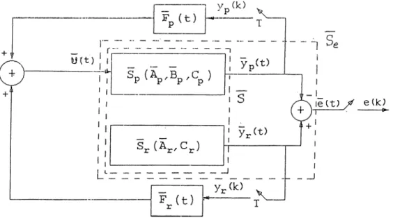
The control structure for the error system Se is defined as
u{t) = Fp{i)yp{k) + Fr{t)yr{k), k T < t < {k + 1)T, (2.7) where T is the sampling period; yp{k) and yr{k) are discrete-time signals obtained by sampling yp{t) and yr{t), i.e., yi{k) = yi(kT), k c Z , i = p,r·, and Fp(t) and F r { t ) are
T-periodic generalized sampled-data hold functions (GSHF); i.e..
CHAPTER 2. RIPPLE-FREE DEADBEAT CONTROL USING GSIIF’S
Figure 2.1. Control Scheme v/ith GSHF Controller
The closed-]oop sampled-data system has the configuration shown in Fig. 2.1, where S and Sq are also indicated. To obtain a discrete-time description of the sampled-
data system in Fig. 2.1, let us define
Xi(k) = Xi{kT), i = p,r, u{k) = u(kT), x(k) = y(k) = xj{k) xj{k) yjXk) yj{k) (2.9) $,· - i = p,r, $ = — diag.{$p , $r}) Tp = r e^p('^-^'>Bpdr, T = [ e^('^-^'>BdT = Jo
Then, the discrete-time augmented system S and the error system Se are described respectively as r / 0 x (k + 1) = ^ x ( k ) + Tu(k) (2.10) y{k) = Cx(k), i x{k + 1) = e(k) = ^ x ( k ) + Tu{k) Dx{k). (2. 11)
CHAPTER 2. RIPPLE-FREE DEADBEAT CONTROL USING GSHF’S
We assume th at the sampling process does not introduce any unobservable modes into Sp and Sr, i.e., ($p,(7p) and (^r ,Or) are observable pairs.
Next, we obtain descriptions of the closed-loop sampled-data and the correspond ing discrete-time systems as follows. First, we rewrite (2.7) as
u(t) = F(t)y{k), k T < t < { k - \ - 1)T, where y(k) is defined in (2.9), and
F{t) = [ Fp(l) Frit) ] . Substituting (2.12) in the expression
i-kT+S
x { k T -b ¿) = e ^^x(kT) -f / e^(^^+ ^-^)5û(r)dr, 0 < 6 < T (2.14)
JkT
which describes the evolution of the state of we obtain
rkT-\-6 x i k TFÔ) - e^^x{kT)F / e^(*^+^-^)5F’(r)i/(^)dT = [e^^-b / e^^^-^">BF{T)CdT]x{kT) Jo where =: ^ 6 ) x { k T ) , rS -,
l(^) =
+ J
e-^(^-^).BF’( r ) C d r , 0 < S < T ' -b Gp{6)Cp Gr{6)Cr " 0 oA-rS with Gi{6)= ( '^^BpFi{r)dT, i = p,r. JoThus the closed-loop sampled-data error system is described by
Se : x ( k T + 6) = §{6)x(kT) ë(kT + 6) = D x { k T + 6) , 0 < 6 < T . (2.12) (2.13) (2.15) (2.16) (2.17) (2.18)
The description of the closed-loop discrete-time error system is obtained from (2.18) with (5 = T as
4 ; + (2.19)
CHAPTER 2. RIPPLE-FREE DEADBEAT CONTROL USING GSHF’S 10 where with $ = $ ( T ) = ”f~ GpCp GyCf 0 Gi = G i { T ) = [ \^^^'^-^)BpFi{T)dT, i = p,r. JO (2.20) (2.2 1)
Having obtained the descriptions for Sq and we now formulate the deadbeat and ripple-free deadbeat control problems as follows.
D e a d b e a t C o n tro l P r o b le m :Find T-periodic generalized sampled-data hold functions Fp{t) and Fr{t) such that for all x{Q)eTZ'^
e[k) = 0, f o r all k > N (2.22)
for some N e .
R ip p le -F re e D e a d b e a t C o n tro l P r o b le m :Find T-periodic generalized sampled- data hold functions Fp{t) and Fr{t) such that for all a;(0)e7^^
e(^) = 0, f o r all t > N T (2.23)
for some N e Z ^ .
2.2
D e a d b e a t C on trol P ro b lem
In this section, the deadbeat control problem is investigated in detail. In the first subsection, the main theorem is stated. The second subsection is devoted to some implications of the main theorem. In the third subsection, the realization of generalized sampled-data hold functions is considered. In the final subsection, geometric solvability conditions are given.
CHAPTER 2. RIPPLE-FREE DEADBEAT CONTROL USING GSHF’S 11
2.2.1
General Solvability Condition
The output of the closed-loop discrete-time error system Se in (2.19) is given by e(k) = D^'^xo, xq = a;(0) = a;(0). (2.24) Thus deadbeat control problem is equivalent to finding Fp(t) and Fr{t) such that
I m C K e r D, f o r all k > N , f or some N e Z+. (2.25) Noting th a t I m C I m for all k > N , (2.25) is equivalent to
C K e r D. (2.26)
The following theorem provides a necessary and sufRcient condition for solvability of the deadbeat control problem.
T h e o re m 2.1 Deadbeat control problem is solvable if and only if there exists X e and Y eKNr^^ such that the following equalities are satisfied simultaneously:
($p + y C p )X =
CpX
=Cr.
(2.27) (2.28)
P ro o f: [N ecessity] Using (2.6) and (2.20), (2.26) can be rewritten as
i N = 0.
-Cp Cr
T GpCp GrCf 0 Defining, $ p = $ p - fGpCp
On = ^ ^ - ^ G r C r ■ l · ^ ^ - ^ G r C r ^ r + ■^■ + G r C r ^ r ^ - \ (2.29) becomesf
-C p Cr 0 = 0, (2.29) (2.30) (2.31)CHAPTER 2. RIPPLHFREE DEADBEAT CONTROL USING GSIIF’S 12
which ill turn implies
and From (2.32), we obtain = 0, CpÜN = C r ^ r ^ . Cp^ Cp^p C p ^ 7 ~^ (2.32) (2.33) (2.34)
where Qp is the observability m atrix of the pair (Cp,$p). Since (Cp,$p) is observable by assumption, so is (Cp, $p) [15], so that Qp has full column rank. Then, (2.34) implies th at
(2.35)
= 0. Noting that $ 7. is nonsingular, we now define
X = Y ^ G p A G r . (2.36)
Then, (2.33) implies (2.28). On the other hand, using (2.35) we obtain
{ % + YCp)X - {^pAGpCp)XAGrCpX = ^ p I l N ^ - ^ + GrCr = { ^ ^ G r C r + ^ ^ - ' ^ G r C r ^ r + . . . + pGrCp (2.37) = + . . . + ^ p G r C r ^ r ^ - ^ + G r C r ^ ^ - ^ ) = =
i.e., (2.27) is also satisfied.
[Sufficiency] Since ((7p, $p) is observable, Gp can be chosen to make $p = $p + GpCp nilpotent; i.e.
(2.38) for some N. Let
CHAPTER 2. RIPPLE-FREE DEADBEAT CONTROL USING GSHF^S
Then, (2.27) and (2.28) imply that
■ 1 - X ' ' ^p GrCr n ^p 0 ' I - X ' 0 I 0 0 0 I and, therefore ' I - X ' ■ |p GrCr 'N ■$p^ 0 ' I - X ' 0 I 0 - 0 _ - 0 I
Hence, from (2.38), we obtain
= [ -C p Cr
-Cp
0 I X I - X 0 I 0 / 0 ■ I - X 0 0 I = 0. $p G^Cr 0 N 13 (2.40) (2.41) (2.42)Thus when (2.27) and (2.28) are satisfied, Gp and Gr can be constructed to satisfy the deadbeat condition (2.26). It remains to show th at given Gp and Gr, Fp{t) and Fr{t) can be solved from (2.21). This is done in section 2.2.3.
2.2.2
Im plications of the M ain Theorem
Following the necessity part of the Theorem 2.1, (2.35) implies th at the closed-loop system is internally stable. Hence, the deadbeat control problem inherently includes the internal stability constraint.
We now elaborate on conditions (2.27) and (2.28) of Theorem 2.1. They together imply th at Gpi^p -b Y C p f X = Cri>i, ¿ = 0 , 1 , . . . . (2.43) In particular, we ha.ve (2.44) ■
Cp
'Cr
Cp{<i>p
+YCp)
X =Cr^r
_
Cp($p -bYCpf-^
_ _ .CHAPTER 2. RIPPLE-FREE DEADBEAT CONTROL USING GSHF’S 14
where r; = max {iip, n,.}. Since the pair (^p,Cp) is observable, then so is [($p + YCp),Cp], BO th a t the coefllcient m atrix on the left-hand side of (2.44) has rank Up.
Similarly, the matrix on the right-hand side has rank n^. This observation leads to the
following corollary of Theorem 2.1.
C o ro lla ry 2.1 A necessary condition for the solvability of the deadbeat control problem is that Up >
Hr-We now turn our attention to the special case of single-output system and reference plant, i.e., when / = 1.
W ithout loss of generality let us assume that the pair ($p,Cp) is in observable canonical form, th at is §p = 0 (f>2 1 4 > 1 (2.45)
Cp
= 0 . . . 0 1 J . (2.46)Also, assume without loss of generality that is in Jordan form with $ r — diag. {«/i, J2·,··■· Jq}^ Xi 1 (2.47) ■ A.· 1 ’■· ’■· (2.48) At 1
where n, = ih·., and A; Xj f o r i / j . Let Ct be partitioned conformably as
Cr =
Cl C2 Cqwhere
Ci = ^i2 · · · , i = 1, 2, . . . , ? .
(2.49)
(2.50) Note that since (4^^> Cr) is observable, we have c,i 7^ 0, ¿ = 1 , 2 , . . . , ? .
I'luaii'/, i>il;
CHAPTER 2. RIPPLE-FREE DEADBEAT CONTROL USING GSIIFH 15
O p r i p 9 r r i p G p — 9 p 2 , K j p — 9t2 9 p i 9 r i (2.51)
We are now ready to prove the following.
C o ro lla ry 2.2 For the single-output case, the deadbeat control problem is solvable if and only if Up > Ur.
P r o o f : [N ecessity] The necessity of the condition Up > has already been stated in Corollary 1.1. Below we provide an alternative proof.
Consider (2.35), which has been shown to be a necessary condition. From the structure of Cp and Gp, it follows that (2.35) is satisfied if and only \i N > Up and
(2.52) th at is
[0
0 - 1 Cl c„ = 0, 1, 2, . . . ' 0 0 ■ 1 0 0 1 0 in (2.29), we get ■ 0 0 9rup 9rripCq 1 0 0 ffr2Ci 9r2Cq 1 0 9ri Cl . . 9r\Cq Jl Jq (2.53) = 0. (2.54) Carrying out multiplications, we obtain the following equivalent equationsCHAPTER 2. RIPPLE-FREE DEADBEAT CONTROL USING GSHF’S 16
Since are nonsingular, (2.55) is equivalent to
rip —1 - g r n p l ) = 0. Now, (2.56) implies <5r($r" - 5 ri$ r '’ - - · · · - grupl) = 0, (2.56) (2.57) where Q r = Cr C r ^ r
is the observability m atrix of the pair ($r,C:·)· Since ( $ ^ ,^ 7·) is observable, (2.57) is satisfied only if
- . .. - grnpl = 0. (2.58)
Finally, from the structure of it follows that degree of the minimal polynomial of is 7ir, so that a necessary condition for (2.58) to be satisfied by some ^,.¿,¿ = 1, 2, . . . , is obtained as rip > Ur.
[Sufficiency] Assuming th at Up > Ur^ let us choose the elements of Gp to satisfy (2.52), and those of Gr to satisfy (2.56). Then is of the form given in (2.53) , and (2.54) is satisfied for any N > rip. This completes the proof.
Another special case that deserves attention is when Cr is square, i.e., when I = rir.
C o ro lla ry 2.3 For the case I = Ur, the deadbeat control problem is solvable if and only if n p > Ur.
P r o o f : Necessity follows from Corollary 2.1. To prove sufficiency, first note that since rank Cr ~ I — 'ih'y Gr is invertible . Now , choose
y =: X ^ r C r ~ ^
-where Cp^ is any right inverse of Cp satisfying CpCp^ = R. Then,
CpX = CpCp^Cr = Cr,
CHAPTER 2. RIPPLEHHiEE DEAD BEAT CONTROL USING GSHF’S
and
17
and
{^p + Y C p ) X = ^ p X + YCr
= $ p X + = X ^ r
so th a t both (2.27) and (2.28) are satisfied.
(2.60)
(2.61)
(2.62)
2.2.3
R ealization s o f G eneralized Sam p led -D ata H old Functions
To complete the proof of Theorem 2.1 we need to show the existence of GSHF’s ^¿(t), i = p, r , which satisfy
r = Gi (2.63)
Jo
for any given G{. This is the well-known controllability problem [16]. Since the pair (Ap^Bp) is controllable, the controllability grammian
rT
-W{ T ) =
is nonsingular [16]. It is then a trivial m atter to show th a t
(2.64)
Fiit) = 5 je ^ p (^ - -* )iy ( r)“ ^(?i, (2.65)
satisfies (2.63).
In the rest of this subsection, we review a method by Araki and Hagiwara[17] to construct piecewise constant GSHF’s Fi{t) which satisfy (2.63). For this, we first recall the following definition.[r7j
CHAPTER 2. RIPPLE-FREE DEADBEAT CONTROL USING GSIIF’S 18
D e fin itio n 2.1 N't (/L,„ 6’,,,') be a controllable vcL·:', where Ap€ and
Bp [ b i. . . brr, J i . A ¿-¿i of integers (iVi, A/o, · · ■ , with Nk > 0 and ^ Nk =
np is said to be the locally minimum controllability indices (LMCI) if
rank [bi . . . Ap^ ' ^ b m] - n p . (2.66)
Let A'^2, . . . , Nra) be a set of LMCI for (Ap, Bp). Define,
N = l.c.m.{Nx, N2, . . . , Nm), (2.67)
T o ^ T l N , Tk = T l N k ,
Let Fi(t) = [ /fcj(t) ], /c = 1, 2, . . . , m; ;■ = 1, 2, . . . , I, where
(2.68)
f kj (t ) = f ' p \ iaTk<t<{iJL + l)Tk] Ai = 0, 1, . . . , iVjt - 1, (2.69)
with being real constants. Then, from (2.63), the column of Gi is expressed as
where. rn N k - l i.U +i)T k - , Si = T . T , h N dr k=\ p=o m N k ~ l _ = E E ( / e^-p(T.-r) J 0 A:=l ^=0 m
= E E
^^^-^-\Tk)bk{Tk)fff, j = l , 2, . . . , l k=l ¡1=0 ^p(Tk) = (2.70) (2.71) and bk(Tk) = ['
h d r =f
e^p^ bk dr. Jo JoEquations (2.70) can be w ritten in compact form as
(2.72)
CHAPTER 2. RIPPLE-FREE DEADBEAT CONTROL USING GSHF’S 19 where E = h i T , ) . . . . . . . . . ] (2.74) and F = [ f kj ], k = j = 1 , 2 , . . . , I, with fkj iNk fkj — f k j ^Nk-1 f L Jokj (2.75)
Prom (2.73), a necessary and sufficient condition for the existence of a solution F for any given Gi is obtained as
rank E = Up. (2.76)
However, as shown in [17], (2.66) implies (2.76) for almost all T.
2.2.4
G eom etric Solvability C onditions
In this subsection, we provide a geometric interpretation(in the sense of Wonham [5]) of the necessary and sufficient conditions (2.27) and (2.28) for solvability of the deadbeat control problem . Let us define the controllability subspace by
B = I m B = < ^ \ T > . (2.77)
Assuming th a t sampling does not introduce any uncontrollable modes into the system, we obtain
B =
671^ X IXy (2.78)
and state the following.
L e m m a 2.1 Conditions (2.27) and (2.28) are simultaneously satisfied by a pair (X, Y) if and only i f there exists a matrix U e and a subspace V C such that
CHAPTER 2. RIPPLE-FREE DEA.DBEAT CONTROL USING GSIIF’S 20
V C Ker D
V ® B =
(2.80) (2.81)
P r o o f : [N ecessity] If (2.27) and (2.28) are satisfied by some pair (X,Y), let
y = Then, (2.27) and (2.28) X ^Ur , U = Y 0 (2.82) ($ + B U C ) V = V ^ r and D V = Q. (2.83) (2.84) Letting V — I m V , the proof follov/s.
[Sufficiency] Let
V =
y (2.85)
be a basis for V, where Vp and y and let U be partitioned as
U = Up Ur (2.86)
where Up, Urf- (2.81) implies th a t y is nonsingular. Let X = VpVr~^ and Y = Up + Ur- Then, it is a simple m atter to show th a t (2.79) and (2.80) imply (2.27) and (2.28).
It has been shown [18] th a t a subspace V C satisfies (2.79) for some m atrix U if and only if it is both $(m od B)- and $|X er(C ')- invariant; i.e., there exists C/i
and U2 such th at
{^-\-BUx)V C V (2.87)
and
C H A P T E R 2. RI PPL E-FREE D E A D B E A T C ONT RO L USING GSIIF’S
Using this resuir, a,nd i.eriinin 2.1, we reach the follo^ving.
21
T h e o r e m 2.2 The deadbeat control problem is solvable if and only if there exists a subspace V C such that
V is ^ \ K e r { C ) — invariant (2.89)
V C K e r D (2.90)
V © < $ 1 r > = (2.91)
P r o o f : [N ecessity] (2.79) implies (2.88), which is equivalent to (2.89). The proof then follows from Lemma 2.1.
[Sufficiency] Let V in (2.85) be a basis for V with K nonsingular. Then,
■ ■ . .
Vr
_ ( K - ' $ r K ) + I 0 ( ^ p V p - V p V r ~ ^ ^ r V r ) , (2.92) th a t is C V + B. (2.93)(2.93) is equivalent to (2.87), and therefore, together with (2.89) implies (2.79). Lemma 2.1 completes the proof.
The geometric conditions of Theorem 2.2 may be useful in developing an algorithm to construct V if it exists, from which X and Y can easily be generated as in Lemma 2.1. Our attem pts so far have failed to come up with such an algorithm. However, it is interesting to compare the above conditions with the solvability conditions of output regulation problem stated by Theorem 8.1 of Wonham[5]. (2.90) and (2.91) are exactly the same in both cases. The only difference is in (2.89), which is replaced by ( $ ,r ) - invariance of V. Remembering th a t $|K er (C')-invariance and ($|r)-invariance concepts are dual, it might be useful to apply the methods and results of geometric approach of Wonham.
2.3
R ip p le - ir e e D e a d b e a t C o n ir o i P r o b le m
In this section, we investigate the ripple-free deadbeat control problem using output feedback and generalized sam pled-data hold functions. In the first subsection, we provide a general solvability result and alternative necessity an d /o r sufficiency theorems. Some examples verifying the results are also given. A special case is the subject of the second subsection.
2.3.1
G eneral Solvability C onditions
CHAPTER 2. RIPPLE-FREE DEADBEAT CONTROL USING GSHF’S 22
From (2.18) and (2.19), the output of the closed-loop sam pled-data error system is obtained as
e{kT-\-6) = D $ ( 6 ) ^ ’^xo, 0 < 6 < T . (2.94) Hence, the ripple-free deadbeat control problem is equivalent to satisfying
D ^ ^ = 0
and
d4 ( 5 ) $ ^ = 0, ¿ e ( 0, r )
for some integer N, where $(<5) and are defined in (2.16) and (2.31).
(2.95)
(2.96)
Let us define
y ( i ) = f\ ^p( ^- ^' ) BpFs (T )dr, 6e[0, T] (2.97) Jo
for some GSIIF Fa{t)€ The following theorem provides necessary and sufficient conditions for solvability of the ripple-free deadbeat control problem.
T h e o r e m 2.3 Ripple-free deadbeat control problem is solvable if and only if there exists and a GSHF F s ( - ) e F ^ ^ ‘ such that
CHAPTER 2. RIPPLE-FREE DEADBEAT CONTROL USING GSHF’S 23
T y(T)Cp )X = A $ ,
Cp[ + Y{S)Cp ]X = ¿ € ( 0,T ).
(2.99)
(2.100)
P r o o f [N ecessity ]: Following the proof of the necessity p art of Theorem 2.1, (2.95) implies (2.33) and (2.35), which in turn, reduces (2.96) to
(7p(e^p(i) + /% ^p(i-^)5p[Pp(r) + F;(r)]Cpdr)i27V$r·^ = (2.101)
Jo
Letting X =■ and noting th a t
Y ( T ) = Gp + Gr, (2.102)
the proof follows from Theorem 2.1.
[Sufficiency]: Choose Gp to make $p — $p + GpCp nilpotent, compute Fp{t) from Gp using the procedure of Section 2.2.3, and let Fr(t) = Fs{t) — Fp{t). Then, Gr = Y { T ) — Gp, and (2.98) and (2.99) imply (2.41) and (2.42), which is the same as (2.95). Finally, using (2.41), left-hand side of (2.96) can be evaluated as
L>l(6')$^ = Dki{6) = 0, I X 0 I I - X 0 I ' o ' ' I - X ' ♦ 0 P 0 0 I (2.103)
where * denotes some m atrix, which is irrelevant to the result. This completes the proof.
We now look at the ripple-free deadbeat control problem from another perspective. Let where Z { 6 ) = \ z l { 6 ) Z j{ 6 ) Zp{6) = + Y{5)Cr, i > 0 (2.104) (2.105)
CHAPTER 2. RIPPLE-FREE DEADBEAT CONTROL USING GSHF’S 24 ibr some X Note th at and
Z.p{S) ■-= ApZp(<5) + B^F,{6)Cr, ^p(O) = X
Zr{,S) = ArZr(S), Zr{0) = In. SO that 'z{S) = AZ{6) + BFs{6)Cr, Z(0) = [ x ^ I The following result is obvious from Theorem 2.3.(2.106)
(2.107)
(2.108)
(2.109)
C o ro lla ry 2.4 Ripple-free deadbeat control problem is solvable if and only if there exists X and a GSHF F3{.) such that the solution of (2.109) satisfies
D Z{S) = 0, i_e[0,T),
I m Z ( T ) C I m Z { 0 ) . (2.110)
Let V = I m Z(0). Then the solution space of (2.109) is exactly the space of solu tions of the closed-loop sam pled-data system S starting in V. referring to the geometric conditions of Section 2.2.4., it follows th at V is exactly the space of states which results in a deadbeat response. Once the state of the overall system is driven into V, then (2 .110) guarantees a ripple-free deadbeat response from then on.
C o ro lla ry 2.5 Ripple-free deadbeat control problem is solvable if there exists X and Fs{s) e TZ{s)”^^‘ with a bounded inverse laplace transform such that
C pX = Cr
{ s I - A p ) - ^ l A B p F3{s)Cp X = X { s I - A r )
(
2.
111)
CHAPTER 2. RIPPLE-FREE D EAD B EAT CONTROL USING GSIIF’S 25
P r o o f : Fellows iinme<lia-teiy irom Theorem 2.3 La'· taking inverse laplace transform of
(2.112).
E x a m p le 2.1 To illustrate the result of Theorem 2.3 and Corollary 2.5, consider a scalar plant whose reference input is generated also by a scalar system; that is Sp = (ap,bp,Cp), Sr = (ar,Cr). Condition (2.111) gives x = Cr/cp, and substituting into (2.1 1 2), we obtain n - n 1 (2.113) fs(^) = -- ---Thus bpCp s ctj. / , ( < ) = <£[0, TJ. OpCp (2.114)
Now, the deadbeat condition requires
= r e^^(^-^'>bpfp{T)dT = (2.115)
Jo <^p
and after choosing fp(t) to satisfy (2.115), fr if) is computed as fr (t) = /«(i) — fp(,l)·
E x a m p le 2.2 Consider a single-output plant with
Ap — ’ 0 1 ' ' 0 ’ 0 - 1 , Bp — 1
1 0
and a single-output reference system with Ar =
Cr =
(2.98) requires that X = 1 0 a /? 0 1 0 0 1 0 , a ,S e 7 l.With X as above a n d Y {6) = yi{S) y2{8) , (2.100) becomes
1 O] l + i/i((J) 1 - e -hi.S) e~^ -s 1 0 a 3 1 0 1 6 0 1 (2.116) (2.117) (2.118) (2.119)
'which TiCucr t h e r i p p l e - f r e e d e a d k e a i control is not possible.
However^ it is easy to check that the deadbeat conditions (2.21) and (2.28) are satisfied with
CHAPTER 2. RIPPLE-FREE DEADBEAT CONTROL USING GSHF’S 26
a =.■ - 1, /3 = ^ y = (1 - e 1 - 1 ■\T
(
2.
120)
E x a m p le 2.3 In this example, we show the existence of a system fo r which the set o f sufficient conditions in corollary 2.5 are not satisfied, while the ripple-free deadbeat control problem is solvable. Consider a second order single output plant represented by
i p = m 0 0 3m ) Bp = Cp = 1 1 , m 7^ 0 (2.121)
and a scalar reference system with
Ar = 2m, Cr = 1. (2.122)
Checking (2.111) and (2.112), we see that sufficient conditions are not satisfied. Next, we can easily show that the GSHF fg it) and X = a;i 1 — xi satisfies (2.98), (2.99) and (2.100), where
fs(t)
=t € [0,T]
(2.123) Xi = [(2 + 3 m T ) e ^ ^ T - 2]/[18((e'"^ - e ^ ^ ^ ) + 6 (e ^^ ^ - 1)],
and T is the solution of
[(2 + 3mT)e3’"^ - 2][50(e2™2’ _ gSmT) io[(eS’”^ - 1)] =
[18((e^^ - + 6(e3'"^ - l)][50(e2’^^ - + (4 + 5mT)e^”^'^ - 4]
(2.124) which is approximately ( ~^^'*-) for negative m, and ( ^ " ^ ) fo r positive m values.
2.3.2
R ipple-Free D ead b eat R egulation
In this subsection, we consider the deadbeat and ripple-free deadbeat control problems for the special case of zero reference input.
CHAPTER 2. RIPPLE-FREE DEADBEAT CONTROL USING GSHF’S 27
in cne absence of a refer'inice in p \u . the rippie-free deadbeat conditions (2.95) and
(2.96) redu·:-: to
C p ^ ^ = 0 (2.125) and C p $ p (i)$ ^ - 0, ¿ e ( 0 ,T ) respectively, where Ip (^ ) = + Gp{S)Cp. Solvability conditions are provided by the following theorem.(2.126)
(2.127)
T h e o re m 2.4 Deadbeat and ripple-free deadbeat regulation problems with internal sta bility are equivalent, and are always solvable.
P ro o f: Following the same argument as in the proof of Theorem 2.1, it follows th at the deadbeat condition (2.125) is equivalent to
$ ^ = 0, (2.128)
which also satisfies the ripple-free deadbeat regulation condition (2.126). (2.128), how ever, implies internal stability, and can always be satisfied by a suitable Gp, which can be realized using a GSHF Fp(t) as discussed in Section 2.2.3.
C h a p ter 3
R IP P L E -F R E E D E A D B E A T C O N T R O L
U S I N G M U L T IR A T E -O U T P U T
C O N T R O L L E R S
In this chapter, we investigate the ripple-free deadbeat control problem using dynamic feedback from multirate-sampled output values. The first section is devoted to problem formulation. In the second section, a solvability condition is presented, and several examples verifying the results are provided. A special case is a subject of the third section.
3.1
F o rm u la tio n o f th e P r o b le m
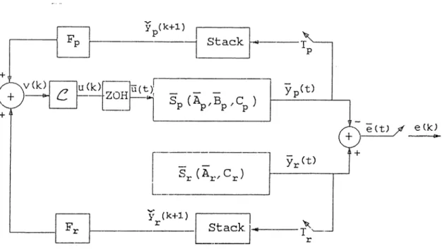
Consider the error system Se of (2.5), which consists of the plant Sp of (2.1) and the reference model of Sr of (2.2). For the purpose of ripple-free deadbeat control of Sp, we consider a MROC operating on sampled values of the plant output and the reference signal as shown in Fig. 3.1.
In the control configuration of Fig. 3.1, the samplers at the outputs of Sp and Sr operate at rates Tp and Tr respectively, where
NpTp = NrTr = T,
28
CHAPTER 3. RIPPLE-FREE DEADBEAT CONTROL USING M RO C ’S 29
Figure 3.1. Control Scheme with M ultirate-O utput Controller
for some integers Np and Nr, and T is the basic sampling period. We define doubly- indexed discrete sequences x f { k , j ) and y f ( k , j ) as
= Xi{kT-I jTi) y i ( k , j ) = V i i k T - I j T i ) for ke Z , j = 0 , 1 , . . . , Ni - 1, z = p, r; and let
Xi{k) = xf{k,0) Vilk) = yf{k,0).
For convenience, we also let
xf(k,N'i) - x f { k + 1,0) = Xi{k-Il) yf{k,Ni) = yf(fc-H l,0) = y ,(/:-|-l).
(3.2)
(3.3)
(3.4)
The output samples y f { k , j ) are stacked into a vector yi{k -f 1) over each basic sampling period, th a t is.
yi{k -f 1) —
y f ( k , N i - l )
J
CHAPTER 3. RIPPLE-FREE DEADBEAT CONTROL USING M ROC’S 30
The diiiCi-eu··. cv/tu.oliv.: C which operates at a. rate compatible v/ith the basic sampling period T is defined as
C : u{k + 1) = Hu( k) v(k), (3-6) where
v(k) — Fpijpik + 1) + Friir^k + 1). (3-7) The control input u{t) to the plant Sp is generated by holding the outputs of C over each basic sampling period, i.e.,
u{t) ^ u{k), k T < t < { k + 1)T.
(3.8)
To obtain a description of the closed-loop sam pled-data system, we first note th at the discrete-time models for Sp and Sr at their own sampling rates are described as
^ p ( k , j + l) = ^ ^ x ^ ( k , j ) + T^u(k), k e .Z, j - 0 , 1 , . . . ,Np - 1 od . Op . and where and d" j)-> x ^ ( k , j + l) = ^ f x f { k , j ) , k c Z , j =
0, l , . . . , Nr - 1
<5“ : 2/r(^hi + l) = Cr x i { k , j ) , , i = p ,r.From (3.9), it follows that
e^^^Bpdr.
i-1
■ \ K i ) = + E ( * h r i « w .
t=rO
and similarly from (3.10)
x i ( k , j ) = i ^ f y x f { k , o ) . Hence, the stacked samples are obtained as
(3.9) (3.10) (3.11) (3.12) (3.13) (3.14)
CHAPTER 3. RIPPLE-FREE DEADBEAT CONTROL USING M RO C ’S 31 г a n , \ Q\ and nd _ Xtp C j i f C, E («?) ( r j ) t = 0 l = p , r , (3.16) (3.17) (3.18)
On the other hand, again from (3.9) and (3.10), the discrete models over the basic sampling period are obtained as
where and о Xp(^k "1” l) — ФрХр(/?) d” Lp'Ui(^k'^ · y^(k) = C p X p ( k ) , (3.19) Ç Xj’l^k 1 ) — Ф^2.7*(А.) ' Уг{к) = CrXrik), (3.20) i = p ,r, (3.21) N p - l
Г,
=E
(3.22) t=0Here, we assume th at the sampling process does not introduce any unobservable and uncontrollable modes into Sp and Sr^ i.e., (Фр,Ср) and (Ф,.,Ст^) are observable pairs and (Фр,Гр) is a controllable pair.
Now, combining (3.6), (3.7), (3.15), (3.16), (3.19) and (3.20), a discrete-time de scription of the closed-loop error system over the basic sampling period T is obtained as
. 3:а{к + 1) = ФаХа{к)
CHAPTER 3. RIPPLE-FREE DEADBEAT CONTROL USING M R O C ’S 32 wiiere Xa(k) = I x ^( k) x j ( k ) $ — Da = $p 0 Tp 0 0 FpQi FrQi H -b FpRj -C p Cr 0 , (3.24)
Finally, to obtain an expression for the continuons-time error signal e(i), we note th at
x( kT- \ - S) = e ^ ^ x ( k T ) +
I
B u {k)d r= e ^ h { k ) + [ e^D) Bu{k)dr (3.25)
= x { k ) + / e^D) [Ax{ k) + Bu { k ) ] d r , 0 < 6 < T , Jo
where A, B and x(k) are as defined in (2.4) and (2.9), and the last equality follows from the fact th a t Noting th a t and Ax{k) 4- Bu{k) = / e^D )Adr. (3.26) Jo Xa(k), (3.27) B ] Xa{k), (3.28) (3.25) can be rew ritten as
(A:r + i) = ( [ In 0 ] + A B dr) xa{ k) .
Substituting Xa{k) = $a^'xa(0) into (3.29) and using e{t) = Dx(t ), we obtain
e(kT
+
¿i)= j?( [
/n^]+ I
^ ^
^a^'Ca(O), 0 < S < T .(3.29)
(3.30)
CHAPTER 3. RIPPLE-FREE DEADBEAT CONTROL USING M ROC’S 33
R ip p ie -F r e e D e a d b e a t C o n tro l P r o b le m : Choose the integers iVp and Nr, and the matrices Fp, Fr and H such th a t for all x-a(C') 7c
e(t) = 0, f o r all t > N T , (3.31) for some N e .
3.2
A S o lv a b ility C o n d itio n
From (3.30), necessary and suiRcient conditions for ripple-free deadbeat response are obtained as and or equivalently, where D In 0 $ a ^ = 0, (3.32) D ( \ A B 1 $ „ ^ = 0, <5e(0,T), Jo *· ·* Qe A B = 0, (3.33) Q e — D DA (3.34)
is the observability m atrix of Se- We note th a t (3.32) is alone the deadbeat condition.
Since the conditions (3.32) and (3.33) involve the controller param eters H, Fp and Fr, they are not practical to use in design. The following theorem provides a sufficient condition in terms of the open-loop system param eters.
T h e o r e m 3.5 Ripple-free deadbeat control problem is solvable in N steps if there exists G € such that
CHAPTER. 3. RIPPLE FREE DEADBEAT CONTROL USING M RO C’S 34 A - i - 4? = 0, where F = Fp ^ ] > as in (S.22).
Proof: For
G=r.
Gp
Gr Dn-1 0 ( $ + F G )^ " ^ : where $p = $p + FpGp and Dn-1 - ^ p - ^ T p G r + ^ ^ - % G r ^ r + · · · + r p G ,$Thus (3.35) and (3.36) are equivalent to
N - 2 r D Dn-1 0 Q e A j ^ - ' ^ ApDN-1 + B p G r^^-'^ 0
=
0,
= 0. where Ap = Ap + BpGp.We now choose Fi, i — p,r^ such th at
G i ----F iQ f^ r '^ , i = p ,r, (3.36) (3.37) (3.38) (3.39) (3.40) (3.41) (3.42) and let II = F p { Q i ^ r % - R i ) .
(3.41) requires th a t Qf have full column rank, which is true provided iVj > pi, i = p^r, where 77,· are the observability indices of ($^, Gp) and ($ ^,G r) respectively. W ith
Ta =
it follows from (3.41) and (3.42) th a t
'T' - 1® y _J- a ^ a a — lup
0
0
0
Lfir0
_
Gp0
Im.
■$p
0
Fp
0
#,·
0
0
GAl>r
0
= $a. (3.43)C-.·:,/.,..csji be rew ritten as
CHAPTER 3. RIPPLE-FREE DEADBEAT CONTROL USING M ROC’S 35
D ^ /n 0 J = 0 Q A a 5 1 = 0, where A = Ap 0 (3.44) (3.45) (3.46) 0 Ar
w ith Ap as defined in (3.40). Due to the special structure of can easily be constructed as ■ O yv-i$r ■ (3.47) ^ a Oyv-i$r 0 0 0 0
It is then a simple job of substitution to show th a t (3.39) and (3.40) imply (3.44) and (3.45) respectively. This completes the proof.
We note as a side-remark th a t since ($ + FG) has only Wp-free eigenvalues and other eigenvalues are not zero, it is imnecessary to check for existence of G for N > np + 1.
It is interesting to compare the solvability conditions of Theorem 3.5 with the necessary and sufficient conditions of Urikurii & N agata [10], who considered ripple-free deadbeat control using constant state feedback under the assumptions th a t m = / and
^p
a 0 (3.43)
is nonsingular for all eigenvalues ¡j, of $r· Urikura & N agata [10] showed th a t, under the stated assumptions, there exists unique matrices X and Y such that
■$p Tp ■ ’ X ' ' X $ r 0 Y Cr Defining V = X
I,
, V = I m V , n,· (3.49) (3.60)CHAPTER 3. RIPPLE-FREE DEADBEAT CONTROL USING M ROC’S 36
thciy proved ’Chat ripirle free deadbeat control witli com tant stivte feedback is possible if and only if
AV d m B K e r Qe. (3.51) In the proof of the sufFicienc}'^ part of the result they constructed a state feedback m atrix G which satisfies (3.35) and (3.36).
On the other hand, with H and G chosen as in the proof of Theorem 3.5 we have from (3.6), (3.7), (3.15), (3.16), (3.41), (3.42), (3.19) and (3.20) u(k + l ) - H u { k ) F p y p ( k 1 ) Friirik + 1) = { H- ^ FpRf)u(k) + FpQ^pXp{k) + FrQfxr(k) = G p [ ^ p X p ( k ) + T p u { k ) ] + G r ^ T X - r i k ) — GpXp{k + 1) + GrXr{k + 1) = Gx{k + 1), (3.52)
so th a t dynamic feedback from m ultirate sampled outputs is equivalent to constant state feedback after the first basic sampling period.
In conclusion, under the assumptions of Urikura & Nagata[10] and H restricted to the form in (3.42), solvability conditions (3.35) and (3.36) are equivalent to the condition (3.51) of Urikura L· Nagata. However, while (3.51) is also necessary for state feedback control, (3.35) and (3.36) are not for dynamic m ultirate output feedback control. Obvi ously, the reason is the freedom in the choice of H.
As a final remark, we are going to show th a t MROC can also strongly stabilize the closed-loop structure under some mild assumptions. For th a t purpose, let us define
A.p — Ap Bp
0 0 Cp 0 (3.53)
C o ro lla ry 3.6 Assuming that
Ap Bp
Cp 0 (3.54)
is full-column rank and Np > T]p, where r}p is the observability index of the augmented system (Ap,C'p), the RFDB control problem, is solvable with strong stability property.
CHAPTER 3. RIPPLE-FREE DEADBEAT CONTROL USING M RO C ’S 37
Procf:3'i< {'■yC-J n and Fy satisfy
I ] =: [ Gp 1 - H ] .
Noting that the appropriate matrices for the augmented system are
=.d $ = ’ <T)'^•*-p 0 pc/ -L p I Q i = ’ Q i R i ' (3.65) (3.56) (3.57) we have
Two assumptions above imply that (S.57) is full·column rank , and hence, (3.55) has a solution for Fp, given any stable II. The proof is complete by Theorem 3.5.
3.3
R ip p le -F ree D e a d b e a t R e g u la tio n
In this section, deadbeat and ripple-free deadbeat regulation problems are considered for the special case of zero reference input.
In the absence of a reference input and togetlier with the choice of II = Fp { Q^^p'^^Tp — Rp ), the sufHcient conditions (3.35) and (3.36) of the ripple- free deadbeat control problem reduce to
Cp($p + T p Gp f - ' ^ - 0, (3.58) and
( ip + 3pC?p)($p + TpGp)^-' = 0. (3.59)
where (3.58) alone is the deadbeat condition. Solvability conditions are provided by the following theorem.
T h e o re m 3.6 Deadbeat and ripple-free deadbeat regulation problems are always solvable with internal stability constraint.
CHAPTER 3. RIPPLE-FREE DEADBEAT CONTROL USING M ROC’S 38
P ro o f: SurLcier.;. cOiiditions (3.58; and (3.5S) can be satisfied b;/ choosing Gp so as to make
(i>p + TpGp)^-^ = 0, (3.60)
which is always possible since ($p,Fp) is a controllable pair, where Gp can be realized by Fp as
Gp = FpQp^p (3.61)
C h a p ter 4
C O N C L U S IO N S
In this thesis, the ripple-free deadbeat regulation and tracking problems are considered for linear, time-invariant systems. The problem is formulated in state-space setting, and is analyzed with two new sam pled-data controllers, namely generalized sampled- d ata hold functions and m ultirate-output controllers. The methods provide simplicity in im plem entation since they are in output feedback form. The necessary and sufficient solvability conditions are stated by theorems in terms of open-loop system parameters.
The main contributions of this thesis are Theorems 2.1, 2.3 and 3.5. Partial results related with the regulation problem already exist in the literature. Theorems 2.4 and 3.6 provide complete results. The solvability conditions are in terms of simultaneous linear/nonlinear m atrix equations involving system transition, input, and output m atri ces of the reference model and the plant. The solvability conditions of Theorem 2.1 are restated in the geometric setting by Theorem 2.2. In other theorems and corollaries, various special cases of the reference model are considered, which help deeply in under standing the solvability conditions. Internal stability and strong stability properties are also investigated.
It is clear th at, there is work to be done towards obtaining system theoretic inter pretations and geometric counterparts of the solvability conditions. This line of research
CHAPTER 4. CONCLUSIONS
40
b3/:kgrou?"^
.bis 1:110313 3ince its deA'^elonmejit requires a difFerent al^iiebraic
A problem which is left open in this thesis is the minimum-time constraint. Our approach is not aimed for obtaining the ripple-free deadbeat response in minimum-time, but rather expressing the solvability conditions in its simplest form.
Another open question is the robustness analysis of the deadbeat and ripple-free deadbeat controllers, which are believed to be quite weak since the controller is highly sensitive to the variations of system parameters.
As a final remark, we note tha,t the alm ost/approxim ate ripple-free deadbeat con trol problems are challenging concepts for further research since their results would be very helpful in industrial applications.
B ib lio g r a p h y
[1] Emami-Naeini, A. and Franklin, G.F., ‘Deadbeat Control and Tracking of discrete Time System s,’ IE E E Trans, on Auto. Control., vol. AC-27, pp. 176-180, Feb. 1982. [2] Kucera, V., ‘The Structure and Properties of Time Optimal Discrete Linear Con
tro l,’ IE E E Trans, on Auto. Control, vol. AC-16, pp.375-377, Aug. 1971.
[3] Leden, B., ‘O utput Deadbeat Control-A Geometric Approach ,’ Int. J. Control, vol. 26, pp.493,507, 1977.
[4] Akashi, H. and Imai, II., ‘O utput Deadbeat Controllers with Stability For Discrete- Time Multivariable Linear Systems,’ IE E E Trans, on Auto. Control, vol. AC-23, No.6, pp.1036-1043, Dec. 1978.
[5] Wonham, W.M., ‘Linear Multivariable Control-A Geometric Approach ,’ New York: Springer-Verlag., 1974.
[6] Kimura, H. and Tanaka, Y., ‘Minimal-Time Minimal-Order Deadbeat Regulator W ith Internal Stability ,’ IE E E Trans, on Auto. Control, vol. AC-26, No. .6, p p .1276-1282, Dec. 1981.
[7] Tou, J.T ., ‘Digital And Sampled-Data Systems Control Systems ’, New York: McGraw-Hill, 1959.
[8] Kucera, V., ‘Discrete Linear ControLThe Polynomial Equation Approach ,’ Aca demic Prague,, 1979.
B IB L IO G R A P H Y
[9] Kucera, V. and Sebek, M., ‘On Deadbeat Controllers IE E E Trans, on Auto. Control, vol. AC-29, No. 8., pp.719-722, Aug. 1984.
[10] Urikura, S. and N agata, A., ‘Ripple-Free Deadbeat Control For Sampled-Data Sys tems ,’ IE E E Trans, on Auto. Control, vol. , C-32, No. 6., pp.474-482, June. 1987. [11] Chammas, A.B. and Leondes, C.T., ‘Part 2. O utput Feedback Controllability ,’ Int.
J. Control, vol. 27, No. 6., pp.895-903, 1978.
[12] Chammas, A.B. and Leondes, C.T., ‘On Finite Time Control of Linear Systems By Piecewise Constant O utput Feedback ,’ Int. J. Control, vol. 30, No. 2., pp.227-234, 1979.
[13] Hagiwara, T. and Araki, M., ‘Design of Stable State Feedback Controller Based on The M ultirate Sampling Of the Plant O utput ,’ IE E E Trans, on Auto. Control, vol. 33. No. 9, pp.812-819, Sept. 1989.
[14] Kabamba, P.T., ‘Control of Linear Systems Using Generalized Sampled-Data Hold Functions ,’ IE E E Trans, on Auto. Control, vol. 33. No. 9, pp.772-783, Sept. 1987. [15] K ailath, T., ‘Linear Systems ,’ Prentice-Hall, Inc., 1980.
[16] Chen, C.T., ‘Linear System Theory and Design ,’ CBS College Publishing, 1984.
[17] Araki, M. and Hagiwara, T., ‘Pole Assignment by M ultirate Sampled-Data Output Feedback,’ Int. J. Control, vol. 44, No. 6, pp.1661-1673, 1986.
[18] Schumacher, J.M ., ‘Regulation Synthesis Using (C,A,B)-Pairs ,’ IE E E Trans, on Auto. Control, vol. .A.C-27, 1982.