Fast and accurate algorithm for the computation of complex linear canonical transforms

Fast and accurate algorithm for the computation

of complex linear canonical transforms

Aykut Koç,1,*Haldun M. Ozaktas,2and Lambertus Hesselink1 1

Department of Electrical Engineering, Stanford University, Stanford, California 94305, USA 2

Department of Electrical Engineering, Bilkent University, TR-06800 Bilkent, Ankara, Turkey

*Corresponding author: aykutkoc@stanford.edu

Received April 1, 2010; revised June 2, 2010; accepted June 30, 2010; posted July 6, 2010 (Doc. ID 126363); published August 5, 2010

A fast and accurate algorithm is developed for the numerical computation of the family of complex linear ca-nonical transforms (CLCTs), which represent the input-output relationship of complex quadratic-phase sys-tems. Allowing the linear canonical transform parameters to be complex numbers makes it possible to repre-sent paraxial optical systems that involve complex parameters. These include lossy systems such as Gaussian apertures, Gaussian ducts, or complex graded-index media, as well as lossless thin lenses and sections of free space and any arbitrary combinations of them. Complex-ordered fractional Fourier transforms (CFRTs) are a special case of CLCTs, and therefore a fast and accurate algorithm to compute CFRTs is included as a special case of the presented algorithm. The algorithm is based on decomposition of an arbitrary CLCT matrix into real and complex chirp multiplications and Fourier transforms. The samples of the output are obtained from the samples of the input in⬃N log N time, where N is the number of input samples. A space–bandwidth prod-uct tracking formalism is developed to ensure that the number of samples is information-theoretically suffi-cient to reconstruct the continuous transform, but not unnecessarily redundant. © 2010 Optical Society of America

OCIS codes: 070.2580, 350.6980, 070.2590.

1. INTRODUCTION

Linear canonical transforms (LCTs) appear widely in op-tics [1–3], electromagnetics, and classical and quantum mechanics [4–6], as well as in computational and applied mathematics [7]. The application areas of LCTs include, among others, the study of scattering from periodic poten-tials [8–10], laser cavities [2,11,12], and multilayered structures in optics and electromagnetics [13].

LCTs with real parameters have received considerably more attention than LCTs with complex parameters [4]. Real linear canonical transforms (RLCTs) are unitary mappings between the elements of Hilbert space of square integrable functions of a variable in R. RLCTs are represented by 2⫻2 unimodular real matrices,

MR=

冋

a b

c d

册

, 共1兲

with determinant equal to 1, where a, b, c, and d are real. The parameter matrices MR form the real symplectic

group Sp共2,R兲 with three independent parameters [14]. RLCTs are of great importance in electromagnetic, acous-tic, and other wave propagation problems since they rep-resent the solution of the wave equation under a variety of circumstances. At optical frequencies, RLCTs can model a broad class of lossless optical systems including thin lenses, sections of free space in the Fresnel approxi-mation, sections of quadratic graded-index media, and ar-bitrary concatenations of any number of these, sometimes referred to as first-order optical systems or quadratic-phase systems [1,15–26].

The extension of RLCTs to complex linear canonical transforms (CLCTs) is rather involved [4,27–29]. The ex-tension is very briefly summarized as follows. When we let the entries of the unimodular transform matrices be complex numbers, we obtain the unit-determinant matri-ces,

MC=

冋

a b

c d

册

, 共2兲

where a, b, c, and d are complex parameters. The matri-ces MCform the complex symplectic group Sp共2,C兲 with

six independent parameters [29]. However, CLCTs repre-sented by this symplectic group can no longer be estab-lished as a unitary mapping between the Hilbert space of square integrable functions in R. Instead, we have a map-ping from the Hilbert space of square integrable functions of a real variable to analytical functions of a complex vari-able on the complex plane in the Bargmann–Hilbert space of square integrable functions [30,31], as established in [4,27–29]. The CLCTs are required to be bounded but not necessarily unitary, in which case we need to represent CLCTs with a semigroup HSp共2,C兲 within the group

Sp_{共2,C兲. More on the mathematical foundations and}

theory of CLCTs can be found in [4,27–29].

Bilateral Laplace transforms, Bargmann transforms, Gauss–Weierstrass transforms [4,27,32], fractional Laplace transforms [33], and complex-ordered fractional Fourier transforms (CFRTs) [34–37] are all special cases of CLCTs. An important special case of CLCTs is the fam-ily of CFRTs. The CFRT is the generalization of the frac-tional Fourier transform (FRT) where the order of the

transformation is allowed to be a complex number, and consequently the abcd matrix elements are in general complex. The optical interpretation of the CFRT, its prop-erties, and optical realizations can be found in [34–38]. An interesting property of CFRTs is that, in some restricted cases, they can be optically realized by RLCTs [39].

To avoid confusion, we note that a number of publica-tions have used the term complex fractional Fourier

transformation (FT) to refer to a particular generalization

of the FRT [40,41], which is not a complex FRT in the sense of the order parameter being a complex number. The entity referred to as a complex FRT in these publica-tions is distinct from what we refer to as a complex FRT and is actually a special case of real two-dimensional (2D) non-separable or non-symmetrical FRTs. Since such transforms are a special case of 2D non-separable LCTs, their digital computation is covered by the algorithm pro-posed in [42]. To avoid confusion with this important but distinct entity, we will use the term complex-ordered to re-fer to complex FRTs belonging to the class of CLCTs. By developing a general algorithm for CLCTs, we also obtain an algorithm for the important special case of CFRTs.

Given its ubiquitous nature and numerous applica-tions, the fast and efficient digital computation of LCTs is of considerable interest. Many works have addressed the problem of sampling and computation of RLCTs, using both decomposition-based and discrete-LCT-based meth-ods [43–51].

The literature and developments on algorithms for real one-dimensional (1D) and real symmetrical (separable) 2D LCTs are reviewed and summarized in [52]. Recent work has also addressed the computation of the more dif-ficult non-symmetrical (non-separable and non-orthogonal) 2D LCTs, which include anamorphic/ astigmatic cases in which the system does not exhibit symmetry about the optical axis [42]. Thus, an appropri-ate fast algorithm exists for all possible 1D and 2D RLCTs. The purpose of this paper is to cover the case of CLCTs. To our knowledge, there is no algorithm in the lit-erature that efficiently calculates CLCTs or even its most prominent special case, the CFRT.

The distinguishing feature of our approach is the way our algorithm carefully addresses sampling and space– bandwidth product issues from an information-theoretical perspective. Special care is taken to ensure that the out-put samples represent the continuous transform in the Nyquist–Shannon sense during every stage of the algo-rithm so that the continuous transform can be fully recov-ered from the samples. Despite the highly oscillatory na-ture of the integral kernel, we carefully manage the sampling rate so as to ensure that the number of samples used is sufficient, but not much larger than the space– bandwidth product of the input signal so that the algo-rithms are as efficient as possible. The straightforward method of sampling the input field and the kernel, and then calculating the output field, is not suitable for sev-eral reasons. First of all, due to the highly oscillatory na-ture of the integral kernel, a naive application of the Ny-quist sampling theorem to determine the sampling rate would result in an excessively large number of samples and inefficient computation. On the other hand, ignoring the oscillations of the kernel and determining the

sam-pling rate according to the input field alone may cause under-representation of the output field in the Nyquist– Shannon sense. This unacceptable situation arises due to the fact that the particular 2D LCT that we are calculat-ing may increase the space–bandwidth product in one or both of the dimensions. If we do not increase the number of samples that we are working with, so as to compensate for this increase, there will be information loss and we will not be able to recover the true transformed output from our computed samples. The computation of CLCTs involves a number of issues which do not arise in the case of RLCTs. The decompositions employ complex chirp mul-tiplications (CCMs) whose effect on the Wigner distribu-tion (WD) must be clarified to ensure proper space– bandwidth tracking and control.

Complex-parametered LCTs allow several kinds of op-tical systems to be represented, including lossy as well as lossless ones. When complex parameters are involved, LCTs may no longer be unitary and boundedness issues may arise. The decomposition of general CLCTs into Fou-rier transforms and real and imaginary CMs allows us to derive conditions on the transform parameters that en-sure boundedness.

We also need to find the conditions under which

HSp共2,C兲 can be constructed as a mapping from R→R.

This is because we are interested in optical applications of CLCTs where the inputs and outputs are functions of real spatial variables. Such CLCTs which map functions over Hilbert spaces from the real line to the real line are called

passive CLCTs in [27], whereas CLCTs that map

func-tions from the real line to analytical funcfunc-tions on complex Bargmann–Hilbert spaces are called active CLCTs. Thus the eligible parameters also depend on how the HSp共2,C兲 semigroup is constructed for R→R. Wolf derived the pa-rameter spaces for which the CLCTs represent a mapping from R→R and the output is bounded [27]. However, this construction excludes some optically important special cases like Gaussian apertures. The decompositions we use allow the derivation of conditions which do not exclude Gaussian apertures. The specification of such conditions was not necessary in the RLCT case.

The paper is organized as follows. In Section 2, we give the fundamental definitions and properties of both RLCTs and CLCTs. Section 3 presents some mathematical pre-liminaries that we use in the derivation of our algorithm and review some special and important CLCTs in optics. In Section 4, we present a careful analysis of every pos-sible case the complex transform matrix may assume and present fast algorithms based on decompositions into gen-eralized CMs, real scalings, and FTs. We also determine whether a given CLCT represents an optically possible bounded input-output relationship from the real line to the real line. Numerical examples to demonstrate the ac-curacy of the algorithm are given in Section 5. Finally we conclude in Section 6.

2. LINEAR CANONICAL TRANSFORMS

We first recall the definition of RLCTs and discuss the group theoretical structure of RLCTs. Then we will give the definition of CLCTs and explain its group theoretical structure.

The RLCT of f_{共u兲 with real parameter matrix M}Ris

de-noted as fM_R共u兲=共CM_Rf兲共u兲,

共CM_Rf兲共u兲 =

冕

−⬁

⬁

KR共u,u⬘兲f共u⬘兲du⬘,

KR共u,u⬘兲 = e−i␲/4

冑

␤ exp关i␲共␣u2− 2␤uu⬘+␥u⬘2兲兴, 共3兲

where␣, ␤, and ␥ are real parameters independent of u and u

⬘

and whereCM_Ris the RLCT operator. The

trans-form is unitary. The 2⫻2 matrix M whose elements are

a , b , c , d represents the same information as the three

pa-rameters␣, ␤, and ␥ which uniquely define the LCT,

MR=

冋

a b c d

册

=

冋

␥/␤ 1/␤ −␤ + ␣␥/␤ ␣/␤

册

=

冋

␣/␤ − 1/␤ ␤ − ␣␥/␤ ␥/␤

册

−1 . 共4兲 The unit-determinant matrix MR belongs to the class of

unimodular matrices. From a group theoretical point of view RLCTs form the three-parameter symplectic group

Sp共2,R兲.

The CLCT of f共u兲 with a complex parameter matrix MC

is denoted as fM_C共u兲=共CM_Cf兲共u兲,

共CMCf兲共u兲 =

冕

−⬁ ⬁

KC共u,u⬘兲f共u⬘兲du⬘,

KC共u,u⬘兲 = e−i␲/4

冑

␤¯ exp关i␲共␣¯u2− 2␤¯uu⬘+␥¯u⬘2兲兴, 共5兲

where␣¯, ␤¯, and ␥¯ are complex parameters independent of

u and u

⬘

and whereCM_Cis the CLCT operator. MCagain

has a unit determinant and is given by

MC=

冋

a b c d

册

=

冋

ar+ iac br+ ibc cr+ icc dr+ idc

册

=

冋

␥¯/␤¯ 1/␤¯ −␤¯ + ␣¯␥¯/␤¯ ␣¯/␤¯

册

, 共6兲 where ar, ac, br, bc, cr, cc, dr, and dcare real numbers. The

overbar in the parameters␣¯, ␤¯, and ␥¯ is to emphasize that these parameters are now complex, corresponding to a to-tal of six real parameters: ␣¯=␣r+ i␣c, ␤¯=␤r+ i␤c, and ␥¯

=␥r+ i␥c. In terms of these parameters the kernel KCcan

be rewritten as KC共u,u⬘兲 = e−i␲/4

冑

␤r+ i␤cei␲共␣ru 2_−2␤ ruu⬘+␥ru⬘2兲_e−␲共␣cu2−2␤cuu⬘+␥cu⬘2兲_. 共7兲 The bidirectional relationship between the␣¯, ␤¯, ␥¯ param-eters and the matrix entries are given as follows:

␣r= drbr+ dcbc b_r2+ b_c2 , ␣c= dcbr− drbc b_r2+ b_c2 , ␤r= br br2+ bc2 , ␤c= − bc br2+ bc2 , ␥r= arbr+ acbc b_r2+ b_c2 , ␥c= acbr− arbc b_r2+ b_c2 , 共8兲 ar= ␤c␥c+␤r␥r ␤r 2_+␤ c 2 , ac= ␤r␥c−␤c␥r ␤r 2_+␤ c 2 , br= ␤r ␤r 2_+␤ c 2, bc= −␤c ␤r 2_+␤ c 2, dr= ␤c␣c+␤r␣r ␤r 2_+␤ c 2 , dc= ␣c␤r−␣r␤c ␤r 2_+␤ c 2 . 共9兲

3. PRELIMINARIES

A. Wigner Distributions

Here we will review the relationship between LCTs and the WD, which will aid us in understanding the effects of the elementary blocks used in our decompositions. The WD, Wf共u,␮兲, of a signal f共u兲 can be defined as follows

[53,54]:

Wf共u,␮兲 =

冕

−⬁ ⬁

f_{共u + u}⬘/2_兲fⴱ_{共u − u}⬘/2_兲e−2␲i␮u⬘du⬘. _共10兲 Roughly speaking, W共u,␮兲 is a function which gives the distribution of the signal energy over space and fre-quency. Its integral over space and frequency, 兰−⬁⬁兰−⬁⬁W共u,␮兲dud␮, gives the signal energy.

Let f denote a signal and fMbe its LCT with parameter

matrix M. Then, the WD of fMcan be expressed in terms

of the WD of f as [1]

WfM共u,␮兲 = Wf共du − b␮,− cu + a␮兲. 共11兲 This means that the WD of the transformed signal is a linearly distorted version of the original distribution. The Jacobian of this coordinate transformation is equal to the determinant of the matrix M, which is unity. Therefore this coordinate transformation does not change the sup-port area of the WD. The invariance of the supsup-port area means that LCTs do not concentrate or deconcentrate en-ergy. The support area of the WD can also be approxi-mately interpreted as the number of degrees of freedom of the signal. Therefore, the number of samples needed to represent the signal does not change after a RLCT opera-tion.

For the purpose of space–bandwidth tracking as em-ployed in our algorithm, we do not require a full charac-terization of the effects of CLCTs on the WD. However, we do need to know the effect of multiplying a function with another function on the WD to derive a space–bandwidth product tracking method for CLCTs. This multiplication property is not required in deriving our previous algo-rithms for RLCTs [42,47], but it will be necessary in our CLCT algorithm. The WD has the following multiplica-tion property [1]: let h共u兲 and f共u兲 be two functions and let

Wh共u,␮兲 and Wf共u,␮兲 be their corresponding WDs. Then h共u兲f共u兲 has the WD given by

冕

Wh共u,␮ − ␮⬘兲Wf共u,␮⬘兲d␮⬘. 共12兲

In other words, when two functions are multiplied, the WD of the resulting function is given by the convolution of the WDs of the initial two functions along the frequency dimension.

It is well known that a nonzero function and its FT can-not both be confined to finite intervals. However, in prac-tice we always work with samples of finite extent signals. We assume that a large percentage of the signal energy, as represented by the WD, is confined to an ellipse with diameters ⌬S in the space dimension and ⌬B in the spatial-frequency dimension, which can be ensured by choosing⌬S and ⌬B suitably. This implies that the space-domain representation is approximately confined to the interval 关−⌬S/2,⌬S/2兴 and that the frequency-domain representation is approximately confined to 关−⌬B/2, ⌬B/2兴. We then define the space–bandwidth product ⌬S⌬B, which is always ⱖ1 because of the uncertainty re-lation. Let us now introduce the scaling parameter s and scaled coordinates, such that the space- and frequency-domain representations are confined to intervals of lengths_{⌬S/s and ⌬Bs. Let s=}

冑

_{⌬S/⌬B so that the lengths} of both intervals become equal to the dimensionless quan-tity

冑

⌬B⌬S, which we denote by ⌬u, and the ellipse be-comes a circle with diameter⌬u. It will not make much difference if we assume that the signal is contained within the smallest square containing this circle. In the new scaled coordinates, signals can be represented in both domains with ⌬u2 _{samples spaced ⌬u}−1 _{apart. We}

will assume that this dimensional normalization has been performed and that the coordinates u and␮ are dimen-sionless.

For a signal with rectangular space-frequency support, the space–bandwidth product is equal to the number of degrees of freedom. This is not true for signals with other support shapes [55]. While we have observed that LCTs do not change the number of degrees of freedom of a sig-nal, they may change its space–bandwidth product. This will be evident when we examine some of the basic special cases of the LCT.

B. CLCTs in Optics and Special CLCTs

Magnification (scaling), FT, real fractional Fourier trans-formation (RFRT), real chirp multiplication (CM), CCM, Gauss–Weierstrass transform, and CFRT are all special cases of CLCTs that have optical realizations. Scaling, FT, RFRT, and CM, which have real parameters, belong to the narrower class of RLCTs and have been reviewed in [47]. In this section, we only review complex-parametered cases that are essential for our development.

1. Complex Scaling (Magnification)

Simple scaling with a real parameter M is an operation which corresponds to optical magnification [47]. If the pa-rameter M is allowed to be complex, we obtain the com-plex scaling operation, which is a special case of CLCTs. With complex scaling, the real axis on which the input function is defined is mapped to a straight line in the com-plex plane passing through the origin and making an

angle arg_{共M兲 with the real axis. The mapping becomes}

R→C. The interpretation of complex scaling in quantum

mechanics has been discussed in [56,57], while an inter-pretation from a signal processing perspective can be found in [58]. However, we are not aware of the realiza-tion and applicarealiza-tion of complex scaling from a purely op-tical point of view.

2. Gaussian Apertures (Complex Chirp Multiplication)

Gaussian apertures, also called soft apertures, are a spe-cial case of CLCTs. They are actually CMs with a complex parameter and are the complex counterparts of CM op-erations. We will hereafter refer to them as CCM. The definition of CCM is similar to the definition of real CM, where we replace the chirp parameter with a purely imaginary complex parameter,

CQiqf共u兲 = Qiqf共u兲 = e ␲qu2 f共u兲, 共13兲 Qiq=

冋

1 0 − iq 1

册

=

冋

1 0 iq 1

册

−1 , 共14兲

where q is real and so iq is a purely imaginary parameter. It essentially behaves like a multiplicative filter where the transmission is dependent on the transverse dimen-sion quadratic-exponentially. To exclude the unbounded case we require qⱕ0.

We now discuss the effect of CCM on the WD. We need this result in order to track and control the space– bandwidth product of CLCTs. This result is not needed in algorithms for RLCTs because there are no CCM stages in RLCTs and is of a considerably different nature than the operations employed there. We use the property given in Eq. (12) with h共u兲=e␲qu2. The WD of h共u兲, denoted by

Wh共u,␮兲, can be obtained by directly using the definition

of the WD [Eq.(10)], Wh共u,␮兲 =

冑

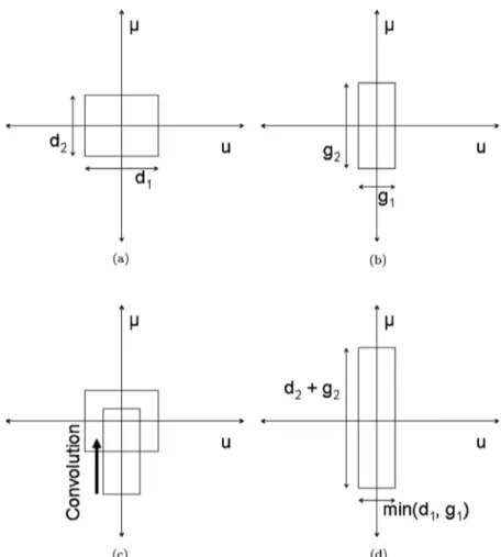
2 − qe 2␲qu2 e共2␲/q兲␮2, q⬍ 0. 共15兲

The WD of the Gaussian function is a 2D Gaussian func-tion in the space-frequency plane. Since q_{⬍0, this} func-tion decays with increasing u and␮. Therefore, we can specify a rectangular region which contains almost all of the energy of the function. We will choose the extent of this rectangle to correspond to plus/minus four standard deviations of the Gaussian in both the space and fre-quency dimensions, which defines a rectangle with extent

g1=

冑

16/␲兩q兩,

g2=

冑

16兩q兩/␲ 共16兲

in the space and frequency dimensions, respectively. When the WD of the input function and the WD of the Gaussian function are convolved along the␮ direction to find the resulting WD of the output function (as illus-trated in Fig.1), the resulting space extent of the support of the output WD will be given by min共d1, g1兲 and the

re-sulting frequency extent will be given by d2+ g2, where d1

and d2are the space and spatial-frequency extent of the

3. Gauss–Weierstrass Transform

The Gauss–Weierstrass transform with parameter t is given by the integral transform [4]

Gtf共u兲 =

冑

1/t

冕

−⬁ ⬁

e−␲共u − u⬘兲2/tf共u⬘兲du⬘. 共17兲 It gives the solution of the heat equation. The complex chirp convolution (CCC) operation, which is a special case of CLCTs, is represented by the transform matrix

Rir=

冋

1 ir

0 1

册

, 共18兲 and is equivalent to convolution by a Gaussian function,

CR_irf共u兲 = Rirf共u兲 = f共u兲 ⴱ ei␲/4

冑

1/r exp共␲u2/r兲. 共19兲

We observe that CCC is the same as the Gauss– Weierstrass transform when we choose the CCC param-eter r = −t. As in the case of the FT, there is again the in-consequential constant phase factor e−i␲/4 _difference

between the two definitions. CCC operations are covered by our algorithm since they are a special case of CLCTs. CCC operations are most conveniently calculated by ex-pressing them as a FT followed by a CCM operation fol-lowed by an inverse FT.

The combined effect of two CCM (or CCC) operations following each other is again a CCM (or CCC) operation, whose parameter is found by summing the parameters of

the two constituent operations. If two CCM operations with real or complex parameters q1 and q2 follow each

other, the equivalent operation is a new CCM operation with parameter q1+ q2. If two CCC operations with real or

complex parameters r1 and r2 follow each other, the

equivalent operation is a new CCC operation with param-eter r1+ r2.

4. CFRT

The ath order RFRT (or simply FRT) is well studied in the literature [1,59–67]. Complex FRTs are FRTs whose order parameter is complex [34–38].

When the order is an imaginary number ib, then we ob-tain the following special case of CLCTs with the trans-form matrix:

F_lcib₌

冋

cosh共b␲/2兲 i sinh共b␲/2兲

− i sinh共b␲/2兲 cosh共b␲/2兲

册

, 共20兲 which again differs only by the factor eb␲/4_{from FRTs as}

commonly defined,

CF_lcibf共u兲 = Flc

ib_{f共u兲 = e}b␲/4_Fib_{f共u兲. 共21兲}

Since FRTs are additive in index, a real-ordered and a purely imaginary-ordered FRT can be combined asFa+ib

=Fa_Fib_{to yield a general CFRT, where the complex order}

may be denoted by ac= a + ib. CFRTs can be optically

real-ized by using thin lenses, free-space propagations, and Gaussian apertures or by combination of Gauss–

Weierstrass transforms with Gaussian apertures [34].

4. ALGORITHM

We now show how given abcd matrices can be decom-posed in a manner that leads to a fast algorithm for the computation of CLCTs. In the most general case, the ma-trix MC is composed of the four complex parameters a , b , c , d, whose real and imaginary parts add up to a total

of eight parameters. These eight parameters are re-stricted by the unimodularity condition on MC, which

re-quires the real part of the determinant to be 1 and the imaginary part to be zero. Because of these two equations, the total number of independent parameters of a general CLCT is 6. These six parameters correspond to the six pa-rameters of the group HSp共2,C兲, which is a six-parameter semigroup of the complex symplectic group Sp共2,C兲. Be-fore giving the main decomposition which covers the gen-eral case, we start with a special case whose treatment is straightforward.

A. b = 0 Case

When b = 0, the unimodularity requirement requires a ⫽0 and the transform output can be written as

共CMCf兲共u兲 =

1

冑

ae

jcy2/2a_{f共y/a兲. 共22兲}

In this case, the output is given by a scaling operation with parameter a followed by a CM operation with pa-rameter −c / 2a. We will restrict ourselves to the case where a is real since only in this case will the scaling op-eration result in a R→R mapping. The case where a is complex produces complex scaling operations and there-fore causes mappings from functions on the real line to functions on the complex plane. This case would require special treatment, which we do not attempt since we are not aware of any optical realization or application of such transforms. Also necessary is the condition Im_共c/a兲, which is necessary to ensure boundedness. In order to have a bounded and R→R mapping, it becomes necessary

for a to be real and Im共c/a兲ⱖ0. Together with the unit-determinant condition, these conditions can be explicitly summarized as follows:

ar⫽ 0,

d = 1/a,

ac= 0,

arccⱖ 0, 共23兲

where the first two are intrinsically required to define any LCT共det MC= 1兲 and the last two are required to obtain a

bounded R→R mapping. When the conditions in 23 are satisfied, the matrix MCcan be decomposed as

MC=

冋

ar 0 c 1/ar

册

=

冋

1 0 c/ar 1

册冋

ar 0 0 1/ar

册

=

冋

1 0 cr/ar 1

册

⫻

冋

1 0 icc/ar 1

册冋

ar 0 0 1/ar

册

. 共24兲

The above decomposition can be used for the fast compu-tation of the special case b = 0.

B. b Å 0 Case

Now, we turn our attention to the more general case in which the following decomposition will be the basis of our fast algorithm: MC=

冋

1 0 − q3r 1

册冋

1 0 − iq3c 1

册冋

0 − 1 1 0

册冋

1 0 − q2r 1

册冋

1 0 − iq2c 1

册

⫻

冋

_{− 1 0}0 1

册冋

_{− q}1 0 1r 1

册冋

1 0 − iq1c 1

册

. _共25兲

This decomposition consists of three imaginary CM and real CM pairs with Fourier/inverse Fourier transform op-erations in between. The imaginary CM and real CM pairs can also be viewed as CCM operations,

MC=

冋

1 0 −共q3r+ iq3c兲 1

册冋

0 − 1 1 0

册冋

1 0 −共q2r+ iq2c兲 1

册

⫻

冋

0 1 − 1 0

册冋

1 0 −共q1r+ iq1c兲 1

册

. 共26兲

The three matrices in the center can also be expressed as a CCC operation, MC=

冋

1 0 −共q3r+ iq3c兲 1

册冋

1 共q2r+ iq2c兲 0 1

册冋

1 0 −共q1r+ iq1c兲 1

册

, 共27兲 which is nothing but the complex version of the well-known CM-CC-CM decomposition [1].

When we multiply out the matrices on the right-hand side of Eq. (25), equate the result to the general CLCT matrix given in Eq. (6), and solve for our decomposition parameters in terms of the CLCT parameters, we get the following: q1r= br− brar− acbc b_r2+ b_c2 , q1c= bcar− bc− brac br2+ bc2 , q2r= br, q2c= bc, q3r= br− brdr− dcbc br2+ bc2 ,

q3c=

bcdr− bc− brdc

b_r2+ b_c2 . 共28兲

Thus, all six parameters of our decomposition have been expressed in terms of the six parameters of the CLCT which we desire to compute. By using Eq.(9), we can also easily calculate the decomposition parameters in terms of the complex␣,␤,␥ parameters if needed. The decomposi-tion in Eq.(25)can also be expressed in operator notation as follows:

CM=Qq_3rQiq_3cFlc−1Qq_2rQiq_2cFlcQq_1rQiq_1c. 共29兲

We now discuss the various cases that arise depending on the values of the parameters. When b⫽0, a separate treatment is required depending on whether a is zero or not. First, consider the case when a = 0. The decomposi-tion parameters given in Eq.(28)become

q1r= br br2+ bc2 , q1c= − bc br2+ bc2 , q2r= br, q2c= bc, q3r= br− brdr− dcbc br2+ bc2 , q3c= bcdr− bc− brdc br2+ bc2 . 共30兲

As discussed in Subsection 3.B.2, the CCM parameters

q1c, q2c, and q3cshould beⱕ0 leading to the conditions

− bc b_r2_{+ b} c 2ⱕ 0, 共31兲 bcⱕ 0, 共32兲 bcdr− bc− brdc br2+ bc2 ⱕ 0. 共33兲

Equations(31)and(32)imply bc= 0 and Eq.(33)becomes brdcⱖ0. When we set bc= 0 in Eq.(30), we obtain the

fol-lowing decomposition parameters:

q1r= 1/br, q1c= 0, q2r= br, q2c= 0, q3r=共1 − dr兲/br2, q3c= − dc/br, 共34兲

with the condition brdcⱖ0. The decomposition we should

use in this case therefore can be expressed as

MC=

冋

1 0 −共1 − dr兲/br 1

册冋

1 0 idc/br 1

册冋

0 − 1 1 0

册冋

1 0 − br 1

册

⫻

冋

0 1 − 1 0

册冋

1 0 − 1/br 1

册

. 共35兲

We now turn our attention to the case b_{⫽0 and a⫽0.} The decomposition given in Eq. (25)and the decomposi-tion parameters given in Eq.(28)are applicable. The be-low three conditions should be satisfied to have a bounded and R→R mapping:

bcⱕ 0, bcar− bracⱕ bc,

bcdr− brdcⱕ bc, 共36兲

which can be equivalently expressed in terms of the ␣,␤,␥ parameters,

␤cⱖ 0,

␣cⱖ␤c,

␥cⱖ␤c, 共37兲

which depends only on the imaginary parts. This is ex-pected since RLCTs are always bounded and unitary, and it is the imaginary parts that are involved in issues of boundedness. These conditions are derived by restricting the parameters of the Gaussian aperture steps in the CLCT decompositions we employ. There are no such con-ditions required for RLCTs. However, these constraints are crucial for the computation of CLCTs. To better illus-trate these conditions, we summarize them in Table1.

The special case b = 0 requires the computation of only real CM and CCM and a real scaling operation. The de-composition for the general case includes CMs and FTs. CMs require only N multiplications and can be done in ⬃N times. The FT and inverse FT can be computed in ⬃N log N times by using the fast Fourier transform (FFT) algorithm. We also note that the scaling operation merely changes the sampling interval in the sense of reinterpre-tation of the same samples with a scaled sampling inter-val, in a manner which corresponds to scaling of the un-derlying continuous signal. Thus the cost of the scaling

Table 1. Summary of the Conditions to Have Bounded R \ R CLCTs

Case 1 Case 2 Case 3

b = 0 b_{⫽0 and a=0} b_{⫽0 and a⫽0}

ar⫽0 bc= 0 bcⱕ0

d = 1 / a b_rd_cⱖ0 b_ca_r− b_ra_cⱕbc

ac= 0 bcdr− brdcⱕbc

operation is minimal and not of consequence since it amounts only to a reinterpretation of the samples. There-fore, the overall CLCT can be computed in ⬃N log N times. To ensure that the number of samples required to represent the function is sufficient in the Nyquist– Shannon sense at each step of the decomposition, we will track the space–bandwidth representation of the function by using the WD and increase the sampling rate when necessary. We will do this with the help of the procedures summarized in [47] for real steps and with the help of Fig.

1 and the discussion given in Subsection 3.B.2 for the complex components. Since the FRT corresponds to rota-tion and the scaling operarota-tion only to a reinterpretarota-tion of the samples, these steps never require us to increase the number of samples. CMs, however, require careful han-dling of the space–bandwidth and sampling issues.

Finally, we summarize our algorithm and the associ-ated space–bandwidth product tracking and sampling control methodology for the most general case. [For the

b = 0 and b⫽0, a=0 special cases, this procedure can be

easily simplified to correspond to the simpler decomposi-tions in Eqs. (24) and (35), respectively.] Whenever the current number of samples will not be sufficient to fully represent the operated-on signal in the Nyquist–Shannon sense, an increase in the number of samples is required prior to performing the operation.

1. We will use Esand Efto denote the spatial and

fre-quency extent of the function as we go through the stages of the algorithm. We assume that the initial space-frequency support is a square of edge length⌬u so that at the beginning Es= Ef=⌬u, and the signal can be

repre-sented with EsEf=⌬u2 samples.

2. The first step of the decomposition is the first CCM with parameter q1c. We use Eq.(16)to obtain the space

and frequency extent of the Gaussian function, which we denote by Gs1and Gf1, respectively. Esand Efare changed

according to Es→min共Es, Gs1兲 and Ef→Es+ Gf1. The

re-quired number of samples then becomes Es⫻Efwhich are

taken in the interval 关−⌬Es/ 2 ,⌬Es/ 2兴 with a spacing of

1 / Efapart from each other. This may or may not require

an increase in the number of samples depending on whether the new Es⫻Efproduct is bigger than the

start-ing number of samples,⌬u2_{. If an increase in the number}

of samples is required, we oversample the signal using an appropriate interpolation scheme and then the CCM op-eration is performed on the input samples.

3. The second step is a CM operation with parameter

q1r. We see that the extent must now become Es→Esand Ef→Ef+兩q1r兩Es. The number of samples required becomes Es⫻共Ef+兩q1r兩Es兲 which will require oversampling with a

factor k = 1 +兩q1r兩Es/ Ef. After this oversampling is

per-formed, the CM operation is performed.

4. We now take the FT of the samples by using the FFT algorithm. We have Es→Ef and Ef→Es since FT only

switches the spatial variable and its spatial-frequency variable. The FT operation does not change the space– bandwidth product of the signal, so oversampling is not required at this stage.

5. Repeat Steps 2 and 3 with the parameters q2c and

q2rcorresponding to subsequent stages of the

decomposi-tion.

6. Repeat Step 4, this time with an inverse FT opera-tion instead of a forward FT operaopera-tion.

7. Repeat Steps 2 and 3 with the parameters q3c and

q3rcorresponding to the final stages of the decomposition

to get the final output samples.

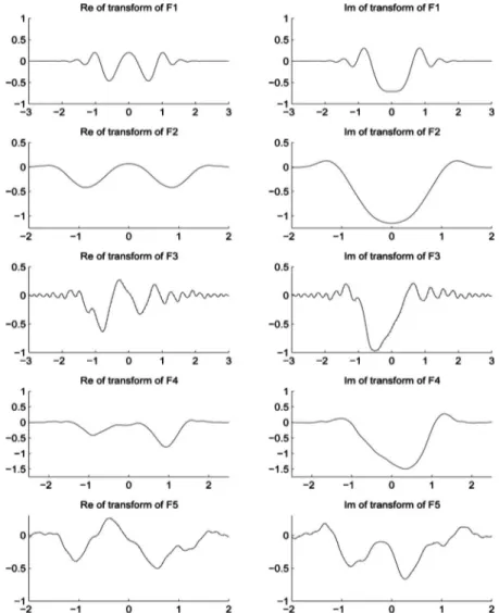
5. NUMERICAL EXAMPLES

We have considered several examples to illustrate the performance of the presented algorithm. We consider the chirped pulse function exp共−␲u2_{− i␲u}2_{兲, denoted by F1,}

and the trapezoidal function 1.5 tri共u/3兲−0.5 tri共u兲, de-noted by F2 关tri共u兲=rect共u兲ⴱrect共u兲兴. Since these two functions are well confined to a circle in the space-frequency plane with a diameter of⌬u=8, we take N=82_. Fig. 2. Example function F4.

We also consider the binary sequence 01101010 occupying [⫺8,8] with each bit 2 units in length so that N=162_{. This}

binary sequence is denoted by F3 and the function shown in Fig.2 is denoted by F4, again with N = 162_.

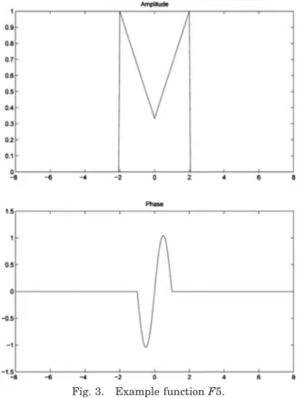
Addition-ally, we also test the example function given in Fig.3with

N = 82 _{that has complex values (i.e., amplitude and}

phase). These choices for ⌬u result in ⬃0%, 0.0002%, 0.47%, 0.03%, and 0.25% of the energies of F1, F2, F3, F4, and F5, respectively, to fall outside the chosen frequency extent. The chosen space extent includes all of the ener-gies of F2, F3, F4, and F5 and virtually all of the energy of F1. We consider three transforms: the first 共T1兲 with parameters 共␣r,␤r,␥r;␣c,␤c,␥c兲=共−2,1.2,−0.9;0.04,0.02,

0.12_{兲, the second 共T2兲 with parameters (1.15,⫺0.14,} ⫺0.1;0.003,0.001,0.002), and the third 共T3兲 with param-eters (_{⫺1.2,⫺0.3,0.1;0.6,0.5,1). The CLCTs T1, T2, and T3} of the functions F1, F2, F3, F4, and F5 have been com-puted both by the presented fast algorithm and by a highly inefficient brute force numerical approach based on Simpson’s numerical integration, which is taken here as a reference.

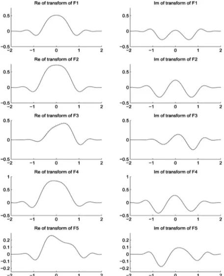
The results for all functions (F1, F2, F3, F4, F5) are plotted in Figs.4and5for transforms T1 and T2,

respec-tively, and are tabulated in Table2for all transforms T1,

T2, and T3. Also shown are the errors that arise when

us-ing the discrete Fourier transform (DFT) in approximat-ing the FT of the same functions, which serves as a refer-ence. (The error is defined as the energy of the difference normalized by the energy of the reference, expressed as a percentage.)

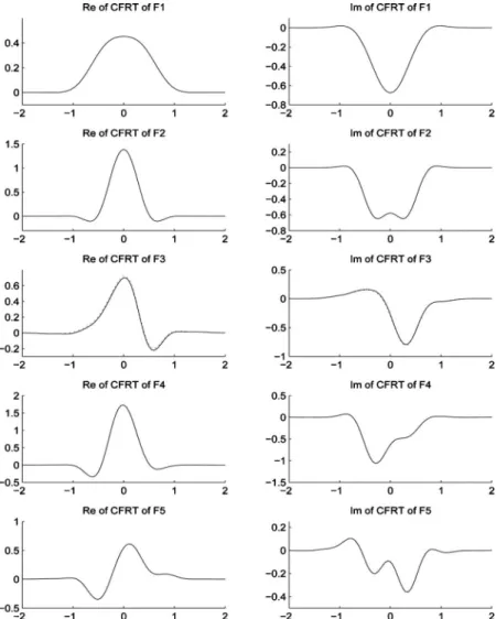
We also tested our algorithm for the CFRT, which is an important special case of CLCTs and the complex exten-sion of the real-parametered FRT. A CFRT with order 0.8− i0.2 is calculated with our algorithm and the refer-ence method and the results are plotted for all functions (F1, F2, F3, F4, F5) in Fig.6and again are tabulated in Table2. The CFRT order 0.8− i0.2 corresponds to CLCT parameters 共␣r,␤r,␥r;␣c,␤c,␥c兲=共0.292,0.9919,0.292;

0.3331, 0.098, 0.3331兲.

Examination of the table shows that our algorithm can accurately compute CLCTs for a variety of transforms and functions. We observe that the main determinant of the error is not the transform, but the function, and more spe-cifically the energy of the function lying outside the as-sumed extent. If we require the error to be further

re-Fig. 4. Transform_{共T1兲 of F1, F2, F3, F4, and F5. The results obtained with the presented algorithm and the reference result have been} plotted with dotted and solid lines, respectively. However, the two types of lines are almost indistinguishable since the results are very close.

duced, we can reduce the excluded energy by increasing the extent and the number of samples involved.

6. CONCLUSIONS

We presented an algorithm for the fast and accurate digi-tal computation of the general family of complex-parametered linear canonical transforms (LCTs). This family of transform integrals can represent a general class of complex quadratic-phase systems in optics. Our approach is based on concepts from signal analysis and processing rather than conventional numerical analysis. With careful consideration of sampling issues, the

num-ber of samples, N, can be chosen very close to the space– bandwidth product of the functions. A naive approach based on the examination of the frequency content of the integral kernels would, on the other hand, result in an unnecessarily high number of samples being taken due to the highly oscillatory nature of the kernels, which would not only be representationally inefficient but also increase the computation time and storage requirements. The transform output may have a higher space–bandwidth product than the input due to the nature of the transform family. Through careful space–bandwidth tracking and control, we can assure that the output samples obtained are accurate approximations to the true ones and that

Fig. 5. Transform_{共T3兲 of F1, F2, F3, F4, and F5. The results obtained with the presented algorithm and the reference result have been} plotted with dotted and solid lines, respectively. However, the two types of lines are almost indistinguishable since the results are very close.

Table 2. Percentage Errors for Different Functions F and Transforms T

T1 T2 T3 CFRT DFT F1 4.12⫻10−6 _2.19⫻10−6 _2.8⫻10−3 _1.24⫻10−5 _2.0⫻10−21 F2 3.73_⫻10−4 _7.1⫻10−3 _1.4⫻10−3 _1.2⫻10−3 _6.2⫻10−4 F3 0.53 0.35 0.26 0.22 1.2 F4 1.2_⫻10−3 _4.96⫻10−2 _2.0⫻10−3 _2.2⫻10−3 _7.1⫻10−2 F5 0.11 0.2 8.0⫻10−3 _6.4⫻10−3 _1.7

they are sufficient (but not unnecessarily redundant) in the Nyquist–Shannon sense, allowing a full reconstruc-tion of the underlying continuous output funcreconstruc-tions. The algorithm takes the samples of the input function and maps them to the samples of the continuous CLCT of this function in the same sense that the fast Fourier trans-form (FFT) implementation of the DFT computes the samples of the continuous FT of a function.

Complex-parametered LCTs allow several kinds of op-tical systems to be represented, including lossy as well as lossless ones. When complex parameters are involved, LCTs may no longer be unitary and boundedness issues may arise. We have identified the conditions for a CLCT to constitute a bounded map from functions on the real axis to functions on the real axis. As a special case of our general CLCT algorithm, we have also obtained an effi-cient and accurate algorithm for complex-ordered frac-tional Fourier transforms (CFRTs).

ACKNOWLEDGMENTS

A. Koç and L. Hesselink gratefully acknowledge support from the Research Laboratories at the General Electric

(GE) Corporation in New York. H. M. Ozaktas acknowl-edges partial support of the Turkish Academy of Sciences.

Note added on proof: We have recently been made

aware of a new work [68] on the subject of fast LCT com-putation.

REFERENCES

1. H. M. Ozaktas, Z. Zalevsky, and M. A. Kutay, The

Frac-tional Fourier Transform with Applications in Optics and Signal Processing (Wiley, 2001).

2. A. E. Siegman, Lasers (University Science Books, 1986). 3. M. J. Bastiaans, “The Wigner distribution function applied

to optical signals and systems,” Opt. Commun. 25, 26–30 (1978).

4. K. B. Wolf, “Construction and properties of canonical trans-forms,” in Integral Transforms in Science and Engineering (Plenum, 1979), Chap. 9.

5. M. Moshinsky, “Canonical transformations and quantum mechanics,” SIAM J. Appl. Math. 25, 193–212 (1973). 6. C. Jung and H. Kruger, “Representation of quantum

me-chanical wavefunctions by complex valued extensions of classical canonical transformation generators,” J. Phys. A 15, 3509–3523 (1982).

7. B. Davies, Integral Transforms and Their Applications (Springer, 1978).

Fig. 6. CFRT with order 0.8− i0.2 of F1, F2, F3, F4, and F5. The results obtained with the presented algorithm and the reference result have been plotted with dotted and solid lines, respectively. However, the two types of lines are almost indistinguishable since the results are very close.

8. D. J. Griffiths and C. A. Steinke, “Waves in locally periodic media,” Am. J. Phys. 69, 137–154 (2001).

9. D. W. L. Sprung, H. Wu, and J. Martorell, “Scattering by a finite periodic potential,” Am. J. Phys. 61, 1118–1124 (1993).

10. L. L. Sanchez-Soto, J. F. Carinena, A. G. Barriuso, and J. J. Monzon, “Vector-like representation of one-dimensional scattering,” Eur. J. Phys. 26, 469–480 (2005).

11. S. Baskal and Y. S. Kim, “Lens optics as an optical com-puter for group contractions,” Phys. Rev. E 67, 056601 (2003).

12. S. Baskal and Y. S. Kim, “ABCD matrices as similarity transformations of Wigner matrices and periodic systems in optics,” J. Opt. Soc. Am. A 26, 2049–2054 (2009).

13. E. Georgieva and Y. S. Kim, “Slide-rule-like property of Wigner’s little groups and cyclic S matrices for multilayer optics,” Phys. Rev. E 68, 026606 (2003).

14. M. Moshinsky and C. Quesne, “Linear canonical transfor-mations and their unitary representations,” J. Math. Phys. 12, 1772–1780 (1971).

15. M. J. Bastiaans, “Wigner distribution function and its ap-plication to first-order optics,” J. Opt. Soc. Am. 69, 1710– 1716 (1979).

16. M. J. Bastiaans, Applications of the Wigner Distribution

Function in Optics, The Wigner Distribution: Theory and

Applications in Signal Processing (Elsevier, 1997), pp. 375– 426.

17. S. Abe and J. T. Sheridan, “Generalization of the fractional Fourier transformation to an arbitrary linear lossless transformation an operator approach,” J. Phys. A 27, 4179– 4187 (1994).

18. S. Abe and J. T. Sheridan, “Optical operations on wavefunc-tions as the Abelian subgroups of the special affine Fourier transformation,” Opt. Lett. 19, 1801–1803 (1994).

19. M. J. Bastiaans and T. Alieva, “Classification of lossless first-order optical systems and the linear canonical trans-formation,” J. Opt. Soc. Am. A 24, 1053–1062 (2007). 20. M. J. Bastiaans and T. Alieva, “Synthesis of an arbitrary

ABCD system with fixed lens positions,” Opt. Lett. 31, 2414–2416 (2006).

21. A. Sahin, H. M. Ozaktas, and D. Mendlovic, “Optical imple-mentations of two-dimensional fractional Fourier trans-forms and linear canonical transtrans-forms with arbitrary pa-rameters,” Appl. Opt. 37, 2130–2141 (1998).

22. T. Alieva and M. J. Bastiaans, “Properties of the canonical integral transformation,” J. Opt. Soc. Am. A 24, 3658–3665 (2007).

23. J. Rodrigo, T. Alieva, and M. L. Calvo, “Optical system de-sign for orthosymplectic transformations in phase space,” J. Opt. Soc. Am. A 23, 2494–2500 (2006).

24. J. A. Rodrigo, T. Alieva, and M. L. Calvo, “Gyrator trans-form: properties and applications,” Opt. Express 15, 2190– 2203 (2007).

25. J. A. Rodrigo, T. Alieva, and M. L. Calvo, “Experimental implementation of the gyrator transform,” J. Opt. Soc. Am. A 24, 3135–3139 (2007).

26. U. Sümbül and H. M. Ozaktas, “Fractional free space, frac-tional lenses, and fracfrac-tional imaging systems,” J. Opt. Soc. Am. A 20, 2033–2040 (2003).

27. K. B. Wolf, “Canonical transformations I. Complex linear transforms,” J. Math. Phys. 15, 1295–1301 (1974). 28. K. B. Wolf, “Canonical transformations II. Complex radial

transforms,” J. Math. Phys. 15, 2102–2111 (1974). 29. P. Kramer, M. Moshinsky, and T. H. Seligman, Complex

Ex-tensions of Canonical Transformations and Quantum Me-chanics, Vol. 3 of Group Theory and Its Applications, E. M.

Loebl, ed. (Academic, 1975), pp. 249–332.

30. V. Bargmann, “On a Hilbert space of analytic functions and an associated integral transform, part I,” Commun. Pure Appl. Math. 14, 187–214 (1961).

31. V. Bargmann, “On a Hilbert space of analytic functions and an associated integral transform, part II,” Commun. Pure Appl. Math. 20, 1–101 (1967).

32. K. B. Wolf, “On self-reciprocal functions under a class of in-tegral transforms,” J. Math. Phys. 18, 1046–1051 (1977).

33. A. Torre, “Linear and radial canonical transforms of frac-tional order,” J. Comput. Appl. Math. 153, 477–486 (2003). 34. C.-C. Shih, “Optical interpretation of a complex-order

Fou-rier transform,” Opt. Lett. 20, 1178–1180 (1995).

35. L. M. Bernardo and O. D. D. Soares, “Optical fractional Fourier transforms with complex orders,” Appl. Opt. 35, 3163–3166 (1996).

36. C. Wang and B. Lü, “Implementation of complex-order Fou-rier transforms in complex ABCD optical systems,” Opt. Commun. 203, 61–66 (2002).

37. L. M. Bernardo, “Talbot self-imaging in fractional Fourier planes of real and complex orders,” Opt. Commun. 140, 195–198 (1997).

38. A. A. Malyutin, “Complex-order fractional Fourier trans-forms in optical schemes with Gaussian apertures,” Quan-tum Electron. 34, 960–964 (2004).

39. L. M. Bernardo, “ABCD matrix formalism of fractional Fou-rier optics,” Opt. Eng. (Bellingham) 35, 732–740 (1996). 40. H. Fan, L. Hu, and J. Wang, “Eigenfunctions of the complex

fractional Fourier transform obtained in the context of quantum optics,” J. Opt. Soc. Am. A 25, 974–978 (2008). 41. D. Dragoman, “Classical versus complex fractional Fourier

transformation,” J. Opt. Soc. Am. A 26, 274–277 (2009). 42. A. Koç, H. M. Ozaktas, and L. Hesselink, “Fast and

accu-rate computation of two-dimensional non-separable quadratic-phase integrals,” J. Opt. Soc. Am. A 27, 1288– 1302 (2010).

43. B. M. Hennelly and J. T. Sheridan, “Fast numerical algo-rithm for the linear canonical transform,” J. Opt. Soc. Am. A 22, 928–937 (2005).

44. B. M. Hennelly and J. T. Sheridan, “Generalizing, optimiz-ing, and inventing numerical algorithms for the fractional Fourier, Fresnel, and linear canonical transforms,” J. Opt. Soc. Am. A 22, 917–927 (2005).

45. H. M. Ozaktas, O. Arıkan, M. A. Kutay, and G. Bozdag˘ı, “Digital computation of the fractional Fourier transform,” IEEE Trans. Signal Process. 44, 2141–2150 (1996). 46. H. M. Ozaktas, A. Koç, I. Sari, and M. A. Kutay, “Efficient

computation of quadratic-phase integrals in optics,” Opt. Lett. 31, 35–37 (2006).

47. A. Koç, H. M. Ozaktas, C. Candan, and M. A. Kutay, “Digi-tal computation of linear canonical transforms,” IEEE Trans. Signal Process. 56, 2383–2394 (2008).

48. F. S. Oktem and H. M. Ozaktas, “Exact relation between continuous and discrete linear canonical transforms,” IEEE Signal Process. Lett. 16, 727–730 (2009).

49. J. J. Healy and J. T. Sheridan, “Cases where the linear ca-nonical transform of a signal has compact support or is band-limited,” Opt. Lett. 33, 228–230 (2008).

50. J. J. Healy, B. M. Hennelly, and J. T. Sheridan, “Additional sampling criterion for the linear canonical transform,” Opt. Lett. 33, 2599–2601 (2008).

51. J. J. Healy and J. T. Sheridan, “Sampling and discretization of the linear canonical transform,” Signal Process. 89, 641– 648 (2009).

52. J. Healy and J. T. Sheridan, “Fast linear canonical trans-forms,” J. Opt. Soc. Am. A 27, 21–30 (2010).

53. F. Hlawatsch and G. F. Boudreaux-Bartels, “Linear and quadratic time-frequency signal representations,” IEEE Signal Process. Mag. 9, 21–67 (1992).

54. L. Cohen, Time-Frequency Analysis (Prentice Hall, 1995). 55. A. W. Lohmann, R. G. Dorsch, D. Mendlovic, Z. Zalevsky,

and C. Ferreira, “Space-bandwidth product of optical sig-nals and systems,” J. Opt. Soc. Am. A 13, 470–473 (1996). 56. B. Simon, “Resonances and complex scaling: A rigorous

overview,” Int. J. Quantum Chem. 14, 529–542 (1978). 57. J. N. Bardsley, “Complex scaling: An introduction,” Int. J.

Quantum Chem. 14, 343–352 (1978).

58. L. Onural, M. F. Erden, and H. M. Ozaktas, “Extensions to common Laplace and Fourier transforms,” IEEE Signal Process. Lett. 4, 310–312 (1997).

59. D. Mendlovic and H. M. Ozaktas, “Fractional Fourier trans-forms and their optical implementation: I,” J. Opt. Soc. Am. A 10, 1875–1881 (1993).

60. H. M. Ozaktas and D. Mendlovic, “Fractional Fourier trans-forms and their optical implementation: II,” J. Opt. Soc. Am. A 10, 2522–2531 (1993).

61. H. M. Ozaktas and D. Mendlovic, “Fourier transforms of fractional order and their optical interpretation,” Opt. Com-mun. 101, 163–169 (1993).

62. H. M. Ozaktas, B. Barshan, D. Mendlovic, and L. Onural, “Convolution, filtering, and multiplexing in fractional Fou-rier domains and their relation to chirp and wavelet trans-forms,” J. Opt. Soc. Am. A 11, 547–559 (1994).

63. L. B. Almeida, “The fractional Fourier transform and time-frequency representations,” IEEE Trans. Signal Process. 42, 3084–3091 (1994).

64. H. M. Ozaktas and D. Mendlovic, “Fractional Fourier op-tics,” J. Opt. Soc. Am. A Opt. 12, 743–751 (1995).

65. H. M. Ozaktas and M. F. Erden, “Relationships among ray optical, Gaussian beam, and fractional Fourier transform descriptions of first-order optical systems,” Opt. Commun. 143, 75–86 (1997).

66. A. Sahin, M. A. Kutay, and H. M. Ozaktas, “Nonseparable two-dimensional fractional Fourier transform,” Appl. Opt. 37, 5444–5453 (1998).

67. A. Sahin, H. M. Ozaktas, and D. Mendlovic, “Optical imple-mentation of the two-dimensional fractional Fourier trans-form with different orders in the two dimensions,” Opt. Commun. 120, 134–138 (1995).

68. J. Healy and J. Sheridan, “Reevaluation of the direct method of calculating Fresnel and other linear canonical transforms,” Opt. Lett. 35, 947–949 (2010).