Hub location under competition

(1)

HUB LOCATION UNDER COMPETITION

A THESIS

SUBMITTED TO THE DEPARTMENT OF INDUSTRIAL ENGINEERING

AND THE GRADUATE SCHOOL OF ENGINEERING AND SCIENCE OF BILKENT UNIVERSITY

IN PARTIAL FULFILLMENT OF THE REQUIREMENTS FOR THE DEGREE OF

MASTER OF SCIENCE

by

Ali İrfan Mahmutoğulları

July 2013

(2)

ii

I certify that I have read this thesis and that in my opinion it is full adequate, in scope and in quality, as a dissertation for the degree of Master of Science.

___________________________________ Assoc. Prof. Bahar Yetiş Kara (Advisor)

___________________________________ Prof. M. Selim Aktürk

______________________________________ Assoc. Prof. Sinan Gürel

Approved for the Graduate School of Engineering and Science

____________________________________ Prof. Dr. Levent Onural

(3)

iii

ABSTRACT

HUB LOCATION UNDER COMPETITION Ali İrfan Mahmutoğulları

M.S. in Industrial Engineering Supervisor: Assoc. Prof. Bahar Yetiş Kara

July 2013

Hubs are consolidation and dissemination points in many-to-many flow networks. The hub location problem is to locate hubs among available nodes and allocate non-hub nodes to these hubs. The mainstream hub location studies focus on optimal decisions of one decision-maker with respect to some objective(s) even though the markets that benefit hubbing are oligopolies. Therefore, in this thesis, we propose a competitive hub location problem where the market is assumed to be a duopoly. Two decision-makers (or firms) sequentially decide the locations of their hubs and then customers choose the firm according to provided service levels. Each decision-maker aims to maximize his/her market share. Having investigated the existing studies in the field of economy, retail location and operation research, we propose two problems for the leader (former decision-maker) and follower (latter decision-maker): (r|Xp) hub-medianoid and (r|p)

hub-centroid problems. After defining them as combinatorial optimization problems, the

problems are proved to be NP-hard. Linear programming models are presented for these problems as well as exact solution algorithms for the (r|p) hub-centroid problem that outperform the linear model in terms of memory requirement and CPU time. The performance of models and algorithms are tested by the computational analysis conducted on two well-known data sets from the hub location literature.

(4)

iv

ÖZET

REKABET ORTAMINDA ADÜ YER SEÇİMİ PROBLEMİ Ali İrfan Mahmutoğulları

Endüstri Mühendisliği Yüksek Lisans Tez Yöneticisi: Doç. Dr. Bahar Yetiş Kara

Temmuz 2013

Ana dağıtım üsleri (ADÜ) her noktadan diğer her noktaya akışın olduğu ağlarda toplama ve dağıtma noktalarıdır. ADÜ yer seçimi problemi, ADÜ’lerin yerlerinin belirlenmesi ve ADÜ olmayan noktaların bu ADÜ’lere atanması olarak tanımlanmaktadır.ADÜ’lerin kullanıldığı sektörlerde çok sayıda firma rekabet halinde olsa da ana akım ADÜ yer seçimi çalışmaları tek karar vericinin amaç fonksiyonları üzerinde yoğunlamıştır. Bu tezde iki karar vericinin olduğu bir ADÜ yer seçimi problemi incelenmiştir. Karar vericiler sırayla ADÜ yerlerini seçmekte ve müşteriler sağlanan hizmet seviyelerine göre bunlardan birini tercih etmektedir. Karar vericiler kendi pazar paylarını enbüyüklemeye çalışmaktadır. Ekonomi, perakende yer seçimi ve yöneylem araştırması alanlarındaki çalışmalarının incelenmesinin ardından lider (ilk karar verici) ve takipçi (sonraki karar verici) için iki farklı problem tanımlanmıştır. Problemler kombinatoriyal eniyileme problmeri olarak tanımlanmış ve karmaşıklık sınıflarının NP-zor olduğu ispatlanmıştır. Bu problemler için doğrusal modeller sunulmuştur. Ayrıca takipçinin problemi için doğrusal modelden daha az bilgisayar hafızası ve çalışma süresine ihtiyaç duyan kesin çözüm algoritmalar geliştirilmiştir. Modeller ve algoritmaların performansı ADÜ çalışmalarında sıkça kullanılan iki veri kümesi üzerindeki sayısal çalışmayla incelenmiştir.

(5)

v

(6)

vi

ACKNOWLEDGEMENT

I would like to express my gratitude to Assoc. Prof. Bahar Yetiş Kara for her guidance and support during my graduate study. Without her supervision, this thesis would not be possible.

I am also grateful to Prof. M. Selim Aktürk and Assoc. Prof. Sinan Gürel for accepting to read and review this thesis. Their comments and suggestions have been invaluable. I also would like to thank my mother Zehra and sister Özlem for their endless love and support every day of my life. My father passed after two months I started Bilkent. I wish he was able to see this thesis.

Without existence of some friends, I could not succeed. Haşim Özlü, Nur Timurlenk, Okan Dükkancı and Cemal İlhan have helped me whenever I need since the very first day I moved to Ankara. I have always felt their unconditional support and trust to me. Feyza Güliz Şahainyazan, Görkem Özdemir and Fırat Kılcı have always been so close

no matter how far they physically are right now. Their help and friendship have been

precious since the first day of my graduate study.

I also would like to thank dear friends and officemates Bengisu Sert, Başak Yazar, Gizem Özbaygın, Meltem Peker and Hatice Çalık. We have so many enjoyable moments together.

I would like to acknowledge financial support of The Scientific and Technological Research Council of Turkey (TUBİTAK) for the Graduate Study Scholarship Program. Finally, I would like to thank Halenur who carries her beauty and goodness wherever she touches. Every single line of this thesis became possible with her love and encouragement.

(7)

vii

LIST OF FIGURES

Figure 2-1: Hotelling's model on a line segment ... 5

Figure 2-2: An example of Drezner’s model when p = 1 and r = 1 ... 9

Figure 2-3: An example where 1-center and 1-centroid do not coincide ... 10

Figure 2-4: An example where a 1-medianoid is not an vertex ... 11

(9)

ix

LIST OF TABLES

Table 2-1: Summary of competitive hub location literature ... 23

Table 4-1: Comparison of H-MED0 and H-MED in terms of size of the models ... 31

Table 4-2: Summary of properties of CAB and TR data sets ... 33

Table 4-3:Optimal solutions of UMApHM and UMApHC in CAB data set ... 34

Table 4-4 Optimal solutions of UMApHM in TR data set ... 34

Table 4-5: Summary of the instances used in the computational study ... 35

Table 4-6: Results of the (r|Xp) hub-medianoid problem on CAB where Xp = UMApHM with α = 0.6 ... 36

Table 4-7: Market share captured by the follower in the optimal solution of H-MED for TR data set where hub set of the leader is UMApHM ... 37

Table 4-8: CPU times of H-MED for TR data set where hub set of the leader is UMApHM ... 38

Table 5-1: Summary of numerical experiments for H-CEN model ... 46

Table 5-2: The percentage of captured flow by the follower for first 5 nodes of CAB data set with p = r = 2 and α = 0.6 calculated by complete enumeration algorithm ... 51

Table 5-3: The percentage of captured flow by the follower for first 5 nodes of CAB data set with p = r = 2 and α = 0.6 calculated by smart enumeration algorithm ... 53

Table 5-4: The percentage of captured flow by the follower for first 5 nodes of CAB data set with p = r = 2 and α = 0.6 calculated by smart enumeration with 50%-bound algorithm ... 54

Table 5-5: Summary of the instances used in the computational study ... 54

Table 5-6: Running times of three algorithms for CAB data with p,r ∈ {2,3} (in CPU seconds) ... 55

Table 5-7: Solution times of smart enumeration and smart enumeration with 50%-bound algorithms for CAB data with α = 0.6 (in seconds) ... 56

(10)

x

Table 5-8: Solution times of smart enumeration and smart enumeration with 50%-bound algorithms for CAB data with α = 0.8 (in seconds) ... 56 Table 5-9: Solution times of smart enumeration with 50%-bound algorithms for TR data set (in CPU seconds) ... 57 Table 5-10: Market share of the follower for CAB data set with α = 0.6 in the optimal solutions of (r|p) hub-centroid, p-hub median and p-hub center ... 58 Table 5-11: CPU time of smart enumeration algorithm with p-hub median bound (in seconds) ... 60

(11)

1

Chapter 1

Introduction

Hubs are consolidation and dissemination points in many-to-many flow network systems. Consolidation generates economies of scale and thus unit transportation cost is reduced between hubs. Hubbing also reduces the number of required links to ensure that each flow is routed to its desired destination. Many applications benefit from hub networks such as airline, cargo and telecom industries. Hub location problem is deciding the location of hubs and allocation of non-hub nodes to the hubs with respect to a given allocation structure and an objective such as minimizing the system-wide operating cost. The facility location literature can be categorized into three groups regarding decision space of the problem. Planar models assume that demand points (or customers) are spread over a plane. The facilities can be located anywhere on this plane. In network models, demand points are regarded as nodes of a graph and facilities can be located on nodes or edges. The third category is discrete models where both demand points and available sites for facilities are nodes of a graph. The majority of hub location literature

(12)

2

falls into discrete facility location category due to practical reasons in cargo, air transportation and telecommunication.

Today, many industries are ruled by a few numbers of competing firms. Such a market is called as an oligopoly (from Greek words oligoi: few and polein: to sell). Hence, market share and profit of a firm is affected by the decision made by itself and other competitors in the market. Also, customer behavior is another concern in oligopolistic markets. Market share is affected by the criteria that customers prefer one firm among others. Competition in oligopolies has been studied by economists to observe optimal decisions (including location) of each competing firm. However, studies considering competition in hub networks are rare in the literature.

Widely speaking, the hub location problem is to determine the location of hubs with respect to a given objective (or at least two objectives in existence of multi-objective optimization problems). A single decision-maker can determine the locations of hubs depending on the parameters: amount of flow and cost of distance between each pairs of nodes, interhub transportation discount factor, allocation strategy (single- or multi-allocation and structure of the network (incomplete, star network etc.). However, in a competitive environment a decision-maker should also consider the decisions made by his/her rivals and the preference of customers. In this study, we consider a duopolistic

market -a special case of oligopoly- where the number of operating firms is two. The

one who makes the location decision formerly is called as the leader and the other one is

the follower.

Then by combining retail location from marketing, spatial competition in economics and location theory in operations research, in this thesis, we propose a discrete Stackelberg hub location problem where each firms makes decisions sequentially. Each decision-maker (or firm) decides the location of hubs and allocation of non-hub nodes to the hubs considering market share maximization.

(13)

3

Chapter 2 presents competitive location and hubbing in the literature. In chapter 3, we propose (r|Xp) hub-medianoid and (r|p) hub-centroid problems as combinatorial optimization problems. In chapters 4 and 5, mathematical models, complexity results, solution techniques and computational experiments for (r|Xp) hub-medianoid and (r|p)

hub-centroid are presented, respectively. Finally, a general discussion and possible

future researches related with these competitive hub location problems are discussed in Chapter 6.

(14)

4

Chapter 2

Competitive Location and Hubbing in

the Literature

In this chapter, we present the literature of competition in economics, competitive location models and hub location problem. Then, we investigate hub location studies in which competition is considered.

2.1 Competition in Economy & Competitive Location Models

Competitive models in economy date back to 19th century. The book Recherches sur les

principes mathématiques de la théorie des richesse (Researches into the Mathematical Principles of the Theory of Wealth) published in 1838 by Cournot is the pioneering

study in the competition in economics [1]. Cournot, a French economist, considers two competing firms operating in the same market. The firms decide the amount of production of a single product. The demand of the product is not known a priori and depends on the total amount of production. Hence, the profit of a firm depends on the amount of production made by itself and the competitor firm. Following Cournot’s

(15)

5

A B

study, another French economist Bertrand considers a duopoly model where the competitors decide the price of a single product in Theorie mathematique de la richesse

sociale (Mathematical theory of social wealth) published in 1883 [2]. In Bertrand’s

model the total demand is known before the decisions and each of the firms aims to maximize its market share or equivalently its total revenue. He considers that each customer prefers the firm that offers lower price to the product.

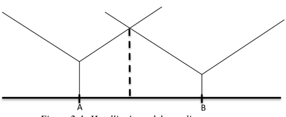
Hotelling presents first competitive model that includes location decisions in 1929 [3]. He considers the location and price decisions of two ice cream vendors operating on a beach. Each customer prefers the vendor that offers lower cost. Cost function includes the price of the ice cream and a linear function of transportation. The demand is assumed to be uniformly distributed on a line segment.

Figure 2-1 is an illustration of Hotelling’s model. The “Y-shaped” functions indicate the cost of buying the ice cream form the vendors A and B. The region between the locations of A and B is called as competitive region. The segment that is located on the LHS of vendor A is called A’s hinterland. Similarly, the segment located on the RHS of the location of B is called as B’s hinterland. The dashed line indicates the point where customers are indifferent between both vendors. The customers located in the hinterland of A and LHS of the dashed line in the competitive region prefers the vendor A. Moving

A’s position towards to B will increase its market share since A’s hinterland increases. Figure 2-1: Hotelling's model on a line segment

(16)

6

Similarly, B has incentive to move towards A. The solution of Hotelling’s model is found as location of both vendors clusters at the center of the market with equal prices. At this equilibrium point, each vendor captures half of the market.

Hotelling’s pioneering work attracted many researchers. Later, Lerner and Singer consider the same model with more than two competitors [4], Smithies considers different customer behaviors [5], and Eaton and Lipsey investigate the equilibrium point on a plane rather than a line segment [6].

In duopoly models presented by Cournot, Bertrand and Hotelling, the decisions of the two firms are made simultaneously. Solutions to these kinds of simultaneous decisions are called as Nash equilibrium (sometimes called as Cournot-Nash equilibrium), after John F. Nash’s great contributions to Game Theory [7]. A Nash equilibrium is a decision vector of all decision-makers where no one can achieve a better objective by changing his/her decision given that other decision-makers do not deviate from their current decisions.

Another streamline research in competitive models deals with not simultaneous but sequential decision making process. The preliminary work of sequential decision making of location is first proposed in Stackelberg’s book Grundlagen der theoretischen

Volkswirtschaftslehre (The Theory of Market Economy) published in 1943 [8]. Since

sequential decision making results in an asymmetry between decision makers, we need to differentiate the identities of decision makers. Stackelberg considers a duopoly where the firm that makes the initial decision is called the leader and the other one as the

follower. Stackelberg’s model has three major assumptions:

 Decisions are made once and for all.  Decisions are made sequentially.

(17)

7

If leader’s decisions are given, the follower’s decisions are made while optimizing his/her own objective. These decisions are called as reaction function of the follower. Since both parties have the complete information of the system, the leader observes the reaction function of the follower. Hence, leader gives the decisions based on this reaction function. These leader-follower situations can be modeled as bilevel optimization problems. Bilevel optimization models consider the follower’s reaction function as an input to the leader’s decisions. Bard [9] and Dempe [10] give detailed discussion on bilevel programming models and solution techniques.

Teitz is the first non-economies scholar who studies sequential location on a line segment in 1968 [11]. His findings are similar to Hotelling’s observations. Moreover, Teitz considers the extension of Hotelling’s model by allowing that each decision maker locates more than one facility. First, Tietz proposes a sequential location model, where one firm, say A, locates two facilities, but the other firm, say B, locates only one facility. The decisions are made by based on short-term maximum gain (referred as “conservative maximization” by Tietz) and continue until equilibrium point is found. A moves first and relocates one of his/her facilities, and then B moves and relocates his/her facility. Later, A relocates, then B and so on ad infinitum. Tietz claims that in such a model the equilibrium point is clustering at the center where at each turn the order of facilities change (for example AAB, ABA, BAA, ABA). At this dancing equilibrium point,

A gets ¾ of the market where B’s share is ¼. Tietz generalizes his results for the case

where A has n facility and B has only one. Then, in resulting equilibrium, A gets

(2n-1)/2n of the market.

Although sequential location models have been studied by economists until 1980s, this topic also attracted OR specialists attention. Some predate works were proposed by Wendell and Thorson [12]; Slater [13]; Wendell and McKelvey [14]; and Hansen and Thisse [15].

(18)

8

Drezner [16] and Hakimi [17] independently propose sequential location problems with an OR point of view and attracted the community’s attention in 1982 and 1983, respectively. They both consider the same competitive environment but decision space is the only difference in their studies. While Drezner considers the decision space as a plane, Hakimi deals with network models. Their problem includes a number of customers with inelastic demand, that is, the amount of demand of each customer is known a priori and does not affected by the decisions of leader and follower. The customers prefer the closest facility to buy a homogenous product. The decision-makers act sequentially, first leader locates p facilities and then the follower locates r facilities. In order to describe Drezner and Hakimi’s contributions, following conventions are necessary. Assume that n customers (or demand points) are located on points

V={v1,v2,…,vn}. The demand of customer i is w(vi). Let D(v,z) = min{d(v,z) : z ∈ Z} where d(v,z) is the distance between v and z for any subset of points Z ⊆ V. The distance between two points is Euclidean distance in two-dimensional plane and the shortest path on a network. Assume that the leader’s and follower’s facilities are located on the set of points Xp={x1,x2,…,xp} and Yr={y1,y2,…,yr} respectively. A customer vi prefers the follower if D(vi,Yr) < D(vi,Xp). Then, the demand captured by the follower can be defined as ( | ) ∑ .

Assume that the leader has already been operating with facilities located on Xp. Then,

(r|Xp) medianoid is the set Yr* such that W(Yr*|Xp) ≥ W(Yr|Xp) for all sets of follower’s possible facility locations Yr. (r|Xp) medianoid is the optimal set of facility locations for the follower to capture the highest market share given Xp.

Similarly, (r|p) centroid is the set Xp* such that W(Yr*(Xp*)|Xp*) ≤ W(Yr*(Xp)|Xp) for all sets of the leader’s possible set of facility locations Xp where Yr*(Xp) is the (r|Xp)

(19)

9

capture the highest market share under the realistic assumption that the follower will respond by (r|Xp) medianoid.

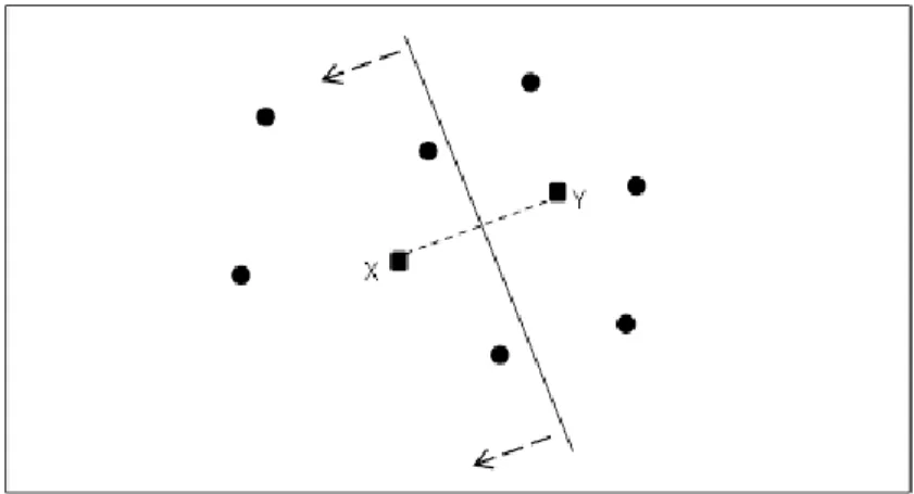
Drezner initially considers a Stackelberg location model where both leader and follower locate one facility each, that is p = 1 and r = 1. Figure 2-2 is an example of Drezner’s model. The demand points are marked with dots on the plane and the leader and the follower located their facilities on point X and Y, respectively. Draw the hyperplane that is perpendicular to the line segment connecting X and Y at the center of the segment. Since customers prefer the closest facility, customers that are on the same half-plane with X prefer the leader and the remaining ones prefer the follower. Then, if X is given, the follower prefers a location Y that is as close as possible to X so as to capture more customers. Hence, the optimal location for the follower’s facility can be searched at the points that are infinitesimally close to X.

Figure 2-2: An example of Drezner’s model when p = 1 and r = 1

Since the demand points are finite, Drezner presents an algorithm that find the (1|X1)

medianoid in O(n log n) time. His algorithm is based on sorting the total amount of demand captured by the follower rotating the position of Y along a circle with center X and an infinitesimal radius. The (1|1) centroid problem is more challenging. Realizing the follower’s optimal response the leader positions X so as to maximize his/her market share. Drezner provided an O(n4 log n) algorithm for the leader’s problem that utilizes

(20)

10

the intersections of hyperplanes for all pairs of demand nodes. Drezner did not study the cases where p > 1 and r > 1. He provided that when p = 1 and r > 1, the (r|p) centroid is on the node with highest demand since the follower can sandwich the leader’s location. He also proposed an O(n2 log n) algorithm to solve for (r|p) centroid when p >1 and r =

1.

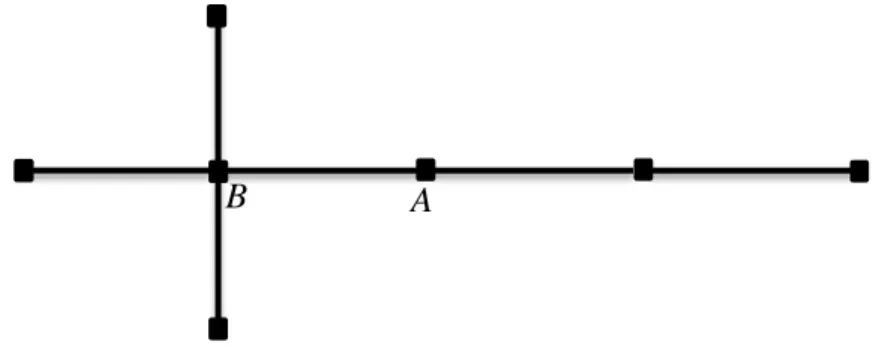
Hakimi proposes medianoid and centroid problems on a network rather than in a plane [17]. He first tries to find general properties of medianoid and centroids by working on some illustrative examples. Hakimi realizes that the centroid problem can be considered as a minimax problem since the leader aims to minimize the amount of demand captured by the follower. However, center and centroid do not necessarily coincide. In Figure 2-3, each node has same demand value. The point A is 1-center of the tree, but not (1|1)

centroid. Moreover, the point B is a (1|1) centroid, but not a 1-center.

Figure 2-3: An example where 1-center and 1-centroid do not coincide

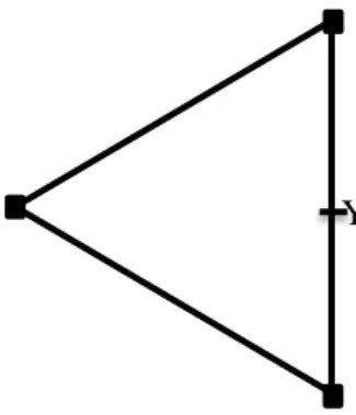
Hakimi also investigates the existence of node optimality of medianoid. His findings also reveal that a medianoid is not necessarily to be a node on the network. In figure 2-4, the leader has already located a facility at one of the edges of an equilateral triangle where the total demand is equally distributed over the vertices. Then, the follower can capture the two-third of the total demand by locating a facility at the center of the side that is opposite to X1.

A B

(21)

11

Figure 2-4: An example where a 1-medianoid is not an vertex

Hakimi cannot find special characteristic of centroids and medianoids. He only proposed that a 1-centroid of a tree network coincides with 1-median. Later, Hakimi proves for the proportional demand case where the leader and the follower proportionally capture the demand of a customer with respect to distance, node optimality exists [18].

Hakimi later proves that both centroid and medianoid problems are NP-hard. His proofs are based on reduction of the dominating set problem and the vertex cover problem to finding (r|X1) medianoid and (1|p) centroid problems, respectively.

Drezner and Hakimi’s influential works attracted many academicians attention in the last three decades. However, most of the studies focus on the medianoid problems since centroid problem is still challenging. ReVelle propose an integer programming formulation for the discrete medianoid problem [19]. His formulation, namely MAXCAP, is based on the maximization of the total demand captured by the follower. In his model, the follower choses p facilities among the set of possible sites J. The follower captures the whole demand ai of node i ∈ I if he/she can provide a strictly better service level than the follower. If both decision-makers have same service level for a customer demand is shared equally between both firms. The decision variables used by ReVelle:

X1 Y

(22)

12

yi = 1 if some server is closer to i than its previous closest server for i ∈ I, and 0 otherwise;

zi = 1 if node i is captured by a server within Ki, that is , at the currently closest server to

i or at a site whose distance from i is equal to the distance from i to its currently closest

server for i ∈ I, and 0 otherwise;

xj = 1 if a facility is sited at j ∈ J, and 0 otherwise; The MAXCAP model is as follows:

maximize ∑ ∑ (2.1) subject to ∑ ∈ _(2.2) ∑ ∈ _(2.3) (2.4) ∑ _(2.5) ∈ { } (2.6)

where Ni is the subset of possible sites that are strictly closer to the demand point i than the closest facility of the leader. Similarly, Ki is the subset of possible sites that are equally close to the demand point i with the closest facility of the leader. The objective (2.1) maximizes the captured demand where constraints (2.2), (2.3) and (2.4) determine whether the demand is totally captured, partially captured or lost. Constraints (2.5) limit the number of opened facility to p. Constraints (2.6) are domain constraints.

Later, Eiselt and Laporte extend the MAXCAP formulation by introducing attraction functions [20]. Serra et al. [21], and Serra and Colome [22] solve the MAXCAP model

(23)

13

for partial demand preferences. Later, Benati addresses the sub-modularity of the objective function of MAXCAP [23], and Benati and Hansen demonstrates that the problem can be modeled as a p-median type problem [24].

For centroid models that are more challenging than medianoid not so many results are obtained so far. Most remarkable work is proposed by Hansen and Labbe [25]. They propose an algorithm that solves (1|1) centroid problem in polynomial time. The algorithm runs in O(n2m2 log mn log D) time where n is the number of nodes, m is the

number of edges and D is the total demand on the network. For p,r > 1 no algorithm is available that runs efficiently. Serra and ReVelle propose two heuristic methods based on the response of the follower for every action of the leader [26].

An interested reader may refer to surveys by Eiselt and Laporte [27] and Daşçı [28] for a detailed discussion for competitive location problems.

2.2 Hub Location Problem

Hubs are special kinds of facilities that are consolidation and dissemination points in many-to-many flow network systems. The flow originating from a point visits one or two hubs before arrival its destination. Since the links between hubs carry high volume of flows, economies of scale is generated on these hubs links and transportation cost (or time) attribute is discounted by a factor α (0 ≤ α ≤ 1).

The hub location problem is to decide locations of hubs and allocations of non-hub nodes to the hubs to optimize a given objective. Two different allocation strategies are considered in the hub location literature. In single-allocation models, the whole incoming and outgoing flow of a node is transferred via a single hub. In multi-allocation case different hubs can be used for transferring the flow of a node.

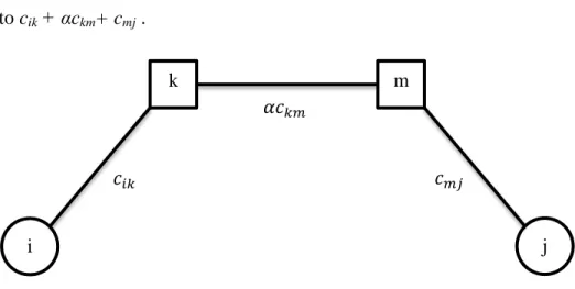
Figure 2-5 gives an example of cost structure in a hub network where squares indicate hubs. Flow from node i to node j first visits the hub to which node i is allocated, say k.

(24)

14

Then, the flow is sent to destination’s hub, say m and finally to the destination which is node j. The total cost of sending one unit of flow from origin to destination consists of collection, transfer and distribution costs where interhub transfer cost is discounted. In the example depicted in Figure 2-5 cost of sending one unit of flow from node i to node j is equal to cik + αckm+ cmj .

Figure 2-5: Cost structure in a hub network

O’Kelly presents the hub location problem where the system-wide transportation cost of the network is minimized by locating p hubs in a single-allocation structure (This problem is later referred as single allocation p-hub median problem) [29,30].

O’Kelly also proposed the first mathematic formulation of the single-allocation p-hub median problem [31]. Define xik as 1 if node is allocated to hub k and 0, otherwise. If a hub is located at node k, then xkk = 1. With these parameters and decision variables, O’Kelly proposes his model as follows:

minimize ∑ ∑ (∑ ∑ ∑ ∑ ) (2.7) subject to ∑ _(2.8) i j k m 𝑐𝑖𝑘 𝛼𝑐_𝑘𝑚 𝑐𝑚𝑗

(25)

15

∑ _(2.9)

∑ _(2.10)

∈ { } (2.11)

The quadratic objective (2.7) minimizes the total collection, distribution and transfer cost of the system. Constraint (2.8) ensures that a node is not allocated to a non-hub node. Constraints (2.9) guaranties that each node is allocated to a single hub. The total number of hub to be opened is p, as in constraint (2.10). Constraint (2.11) is the binary constraint. Constraint (2.8) can be replaced with the following corresponding constraint.

(2.12)

Campbell proposes the first linear formulation for the single allocation p-hub median

problem with n4+n2+n variables of which n2+n are binary and n4+2n2+n+1 constraints

[32]. Later Skorin-Kapov et al. provides a new linear model with n4+n2 variables of

which n2 are binary and 2n3+n2+n+1 constraints [33]. Their model is as follows:

minimize ∑ ∑ ∑ ∑ ( ) (2.13)

subject to (2.9)-(2.12)

∑ _(2.14)

∑ _(2.15)

(2.16)

where xijkm is the fraction of flow from node i to node j that is transferred via hubs k and

(26)

16

Ernst and Krishnamoorthy model the single allocation p-hub median problem as a multi-commodity flow problem [34]. Their formulations require n3+n2 variables of which n2 are binary and 2n2+n+1 constraints. The formulation is as follows:

minimize ∑ ∑ ∑ ∑ ∑ (2.17)

subject to (2.9)-(2.12)

∑ ∑ ∑ _(2.18)

(2.19)

where is the amount of flow originating from node i and visits hubs k and l in that order. and are unit collections and distribution costs, respectively. Constraint (2.18) is the flow balance constraint that ensures that each flow is transferred to its destination via one or two hubs.

The single allocation p-hub median problem is NP-hard. Kara proves that even if the hub locations are given, the remaining allocation decisions are still cannot be solvable with an algorithm that runs in polynomial time [35]. Since the problem is NP-hard, heuristics are widely used to come up with a promising solution to the single allocation

p-hub median problem such as [31].

The multi-allocation p-hub median problem has also attracted attention. Campbell presents the first multi allocation hub model [36]. His formulation is as follows:

minimize (2.13)

subject to (2.10),(2.11) and (2.16)

∑ ∑ _(2.20)

(27)

17

(2.22)

Campbell also states that in absence of capacity each xijkm has a value of 0 or 1 since each flow travels the least cost path through opened hubs. Later, Skorin-Kapov develop a linear model with n4+n variables of which n are binary and 2n3+n2+1 constraints by aggregating constraints (2.21) and (2.22) [33]. Ernst and Krishnamoorthy model the

multi-allocation p-hub median problem based on the idea that they use for the

single-allocation version of the problem [37]. Their model requires 2n3+n2+n variables of which n are binary and 4n3+n+1 constraints.

Some heuristic models are also improved to solve multi-allocation p-hub median

problem. Some examples are can be found in the studies proposed by Campbell [38],

Ernst and Krishnamoorthy [37], and Boland et al. [39].

Although hub location problem under median objective constitutes the main streamline of the literature, other types of objectives are also investigated by the researchers. Another channel of research on hub location problem is the hub location problem with

fixed costs. In the structure of the problem the number of hubs to be opened is

exogenous. The constraint on the number of hubs - constraint (2.10) - is removed and a fixed cost of opening a hub at node k, say fk, is included in the objective function. O’Kelly [40] and Campbell [36] propose mathematical models for the hub location

problem with fixed costs where capacities of hubs are ignored. The capacity constraints

can be included in hub location problem with fixed costs to ensure that the total flow throughout a hub does not exceed a threshold value. Campbell [36] and Aykin [41] present mathematical models for the capacitated version of the problem.

In some applications of hub networks, for example in cargo applications where the cargo should be delivered within a 24-hours period, not only the cost but also service levels are considered. The p-hub center problem is to locate p hub on a network to ensure that the

(28)

18

distance or cost between the most disadvantageous pair of nodes does not exceed a given cover radius.

Campbell proposes the first linear model for the hub location problems with center-type objectives [32]. Kara and Tansel prove that the p-hub center problem is NP-hard by using reduction from the dominating set problem [42]. They also propose different mathematical models for the model. Later, Ernst et al. provide a new formulation for the

p-hub center problem based on the value of maximum collection/distribution distance

between a hub and a non-hub node [43].

Hub covering problem is another version of the hub location problem. There are two

types of hub covering problem: Hub set covering problem and maximal hub covering

problem. Hub set covering problem is to minimize the number of hubs to be located by

ensuring that the distance or cost between each O-D pair does not exceed a given threshold value. On the other hand, maximal hub covering problem is to maximize the total demand that are covered by a given number of hubs.

Campbell is the first researcher who presents mathematical models for different types of hub covering problem [32]. After his contribution, Kara and Tansel study single

allocation hub set covering problem and propose three different linearizations of the

problem [44]. They also worked on the complexity of the problem and conclude that the problem is NP-hard. Later, Ernst et al. provide new formulations of the problem based on the idea that they use for the p-hub center problem [45].

An interested reader may refer to surveys by Campbell et al. [46], Alumur and Kara [47] and Kara and Taner [48] for a detailed discussion of hub location problems.

2.3 Hub Location with Competition

Although the competition in location decisions has been studied in detail, competitive hub location studies in the literature are rare. The first hub location problem with

(29)

19

competition is proposed by Marianov et al. [49]. They propose mathematical models for the follower’s problem where the leader has already been operating the market with existing hubs. First, they assume that the follower will capture the whole demand between nodes i and j if he/she can provide a better or equal service level than the leader. The idea is based on defining a capture set Nij = {(k,l) : cik +αckm +clj ≤ Cij} for all pair of nodes i and j where Cij is the current service level provided by the leader. The number of hubs to be opened by the follower is restricted by p. However, they relax this assumption by redefining the objective function as the total profit made by captured flow and the fixed cost of opening a hub.

They also consider proportional capture levels instead of all-or-nothing type capture. For example, they assume that the leader capture half of the flow between nodes i and j if his/her service levels is between 0.9Cij and 1.1Cij, three-fourth of the flow if his/her service levels is between 0.7Cij and 0.9Cij and captures the whole flow if his/her service level is less than 0.7Cij. Then, the capture sets are redefined as Nij50, Nij75 and Nij100 for the capture levels 50%, 75% and 100%. The mathematical model is provided for the proportion capture case by triplicating the capture variables and constraints. However, due to large number of constraints and variables it is hard to get an optimal solution within reasonable time.

The authors propose a meta-heuristic to solve the problem on AP data set. The heuristic consists of three steps. First, an initial solution is generated by opening hubs based on the marginal improvements obtained by opening a hub at a specific node. Later, a heuristic is used to improve the objective by relocating one hub at each iteration. Finally, to prevent the trap on a local optimal a tabu-search heuristic is used. The efficiency of the heuristic is tested by the randomly generated instances and AP data set with 20, 25, 40 and 50 nodes. They point out that the heuristic yields an optimal solution in most of the instances within seconds. It is also stated that, the LP relaxation of the model and the

(30)

20

branch and bound technique does not yield a fast solution even if the number of nodes is 20.

Wagner criticizes the study by Marianov et al. on his note [50]. Wagner states that the capture sets should be redefined since the follower captures the whole demand in case of a tie when all-or-nothing type capture is considered. When the number of hubs to be opened is equal to the number of existing hubs the follower can get the whole market by location the hubs at the location of existing hubs. Then, Wagner proposes a new capture set where the follower gets nothing in case of equal service levels. Wagner was also able to solve the model optimally up to 50 nodes by eliminating some redundant routes that visit two hubs.

Sasaki and Fukushima propose a new kind of competitive hub location model where the decision space is a plane [51]. The route between any O-D pair on the plane visits only one hub. First, a big firm locates one hub, and then several medium size firms locate their hubs. There is no competition between medium size firms. They state that the problem has a Stackelberg model due to its sequential decision structure.

Sasaki and Fukushima uses logit functions for customer preferences to express the proportional capture in their model. They initially model the problem as a bilevel program and use sequential quadratic programming approach that updates the Hessian at each iteration to solve the problem. They conduct computational experiments on CAB data set and conclude that the big firm gets the highest market share with the advantage of first move.

Sasaki applies the same idea in the study by Sasaki and Fukushima to a discrete environment with some modifications [52]. Her model includes two decision-makers: one leader and one follower. The leader and the follower locate p and q hubs on the network, respectively. The capture rule of the customer is similar to their previous study and each route contains one hub again. In her new problem environment, Sasaki also

(31)

21

considers a threshold value of the captures amount of flow. Her solution methods are complete enumeration and a greedy heuristic that does not perform very well in terms of CPU time when p < q.

Eiselt and Marianov propose another hub location model with competition where an airline transportation company enters a market [53]. It is assumed that some other companies already operate the market. The entrant firm aims to capture as much customer as possible. Customers’ preferences are based on the basic attractiveness of the firms (such as safety record, personal space, quality of the foods etc.), the number of stopover on the trip, cost of the route and time required by the flight. These factors are converted to an attraction function by using a Huff-like model. So, the fractional capture is allowed. They propose a nonlinear mathematical model of the problem which is solved with a two phase meta-heuristics. The first phase, set of available sites is restricted to a smaller set, called as concentration set, and an initial solution is obtained. This initial solution is improved in the second phase by relocation the hubs of the follower.

They test the meta-heuristics with the 25-node version of the AP data set. The computational analysis reveals that follower has a great advantage in the most of the instances and is able to capture 70% of the total customers. Eiselt and Marianov later used a 50-node version of the same data set; however they were not able to solve the problem within reasonable CPU times.

Another hubbing problem with Stackelberg competition is studied by Sasaki et al. [54]. In their problem environment, the decision-makers do not locate hubs but they locate hub arcs. One leader and one competitor airline companies locate qa and qb hub arcs on the network to maximize the total revenue. The leader can capture 0%, 25%, 50%, 75% or 100% of the flow between any O-D pair based on the cost and the travel time of the trip and the remaining customers prefer the follower. They propose a bilevel program of

(32)

22

the model and use a smart complete enumeration scheme that does not perform quick solutions for the instances with large qa and qb to solve the problem. CAB data set is used to test the efficiency of the solution technique. The authors conclude that the geography plays an important role on the location of hubs in the competitive environment.

Although existing studies contribute to hub location and competition literature, both theoretical aspect of the problem and application in industry required much more effort. Therefore, in this thesis, we formally define hub-medianoid and hub-centroid problems by following the terminology used by Hakimi [17] for the analogous competitive location problems in order to motivate the studies in this area. Moreover, we prove that both problems are NP-hard.

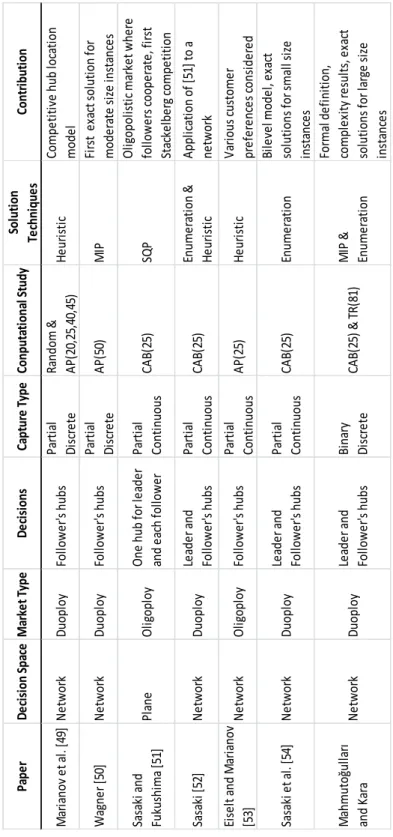
The following table summarizes the paper mentioned above with their contribution to the literature. The last row indicates the contributions made by our study.

(33)

23

Table 2-1: Summary of competitive hub location literature

M ar ia no v et al . [ 49 ] N etw or k D uo pl oy Fo llo w er 's h ub s Pa rti al D is cr ete Ra nd om & A P( 20 ,2 5, 40 ,4 5) H eu ri sti c Co mp eti ti ve h ub lo ca ti on mo de l W ag ne r [ 50 ] N etw or k D uo pl oy Fo llo w er 's h ub s Pa rti al D is cr ete A P( 50 ) M IP Fi rs t ex ac t s ol uti on fo r mo de ra te s iz e in sta nc es Sa sa ki a nd Fu ku sh ima [5 1] Pl an e O lig op lo y O ne h ub fo r l ea de r an d ea ch fo llo w er Pa rti al Co nti nu ou s CA B( 25 ) SQ P O lig op ol is ti c ma rk et w he re fo llo w er s co op er ate , f ir st Sta ck el be rg c omp eti ti on Sa sa ki [5 2] N etw or k D uo pl oy Le ad er a nd Fo llo w er 's h ub s Pa rti al Co nti nu ou s CA B( 25 ) En ume ra ti on & H eu ri sti c A pp lic ati on o f [ 51 ] to a ne tw or k Ei se lt an d M ar ia no v [5 3] N etw or k O lig op lo y Fo llo w er 's h ub s Pa rti al Co nti nu ou s A P( 25 ) H eu ri sti c V ar io us c us tome r pr ef er en ce s co ns id er ed Sa sa ki e t a l. [5 4] N etw or k D uo pl oy Le ad er a nd Fo llo w er 's h ub s Pa rti al Co nti nu ou s CA B( 25 ) En ume ra ti on Bi le ve l mo de l, ex ac t so lu ti on s fo r s ma ll si ze in sta nc es M ah mu toğu lla rı an d Ka ra N etw or k D uo pl oy Le ad er a nd Fo llo w er 's h ub s Bi na ry D is cr ete CA B( 25 ) & T R( 81 ) M IP & En ume ra ti on Fo rma l d ef in iti on , co mp le xi ty re su lts , e xa ct so lu ti on s fo r l ar ge s iz e in sta nc es So lu ti on Te ch ni qu es Co nt ri bu ti on Pa pe r D ec isi on S pa ce M ar ke t T yp e D ec isi on s Ca pt ur e Ty pe Co np ut at io na l S tu dy

(34)

24

Chapter 3

Problem Definition

Given a network G=(N,E) where N is the set of nodes and E is the set of edges, let wij be the flow between nodes i and j for all i,j ∈ N and cij be the transportation cost of a unit flow from node i to node j for all i,j ∈ N . The interhub transportation cost is discounted by a factor α, 0 ≤ α ≤ 1. (We use <G=(N,E), wij, cij, α> nomenclature to refer this many-to-many flow network in the remainder of the thesis.) The leader and follower want to enter a market with prespecified number of hubs. Say p and r be the number hubs to be opened by the leader and follower, respectively. We assume that both p and r are grater or equal to 2 since otherwise there is no interhub link and economies of scale is not generated. Let H ∈ N be the subset of nodes that are available to locate a hub. The customers prefer the leader or follower with respect to provided service levels. Service level is defined as the cost of routing the flow from a node to its destination via hubs. A customer prefers the follower if the service level provided by the follower is strictly less than the one provided by the leader, otherwise the demand is captured by the leader. Ties are broken in the advantage of the leader in case of equal service levels since the

(35)

25

customer has already operating with the leader when the follower enters the market and the customer has no incentive to deviate from the current position.

First, assume that the leader has already operating the market with hubs located at a subset of nodes Xp={x1,x2,…,xp}, Xp ⊆ H. The flow originated from node i visits one or two hubs before arrival to its destination node j. Therefore, we can easily compute the service level, say βij, provided by the leader for the flow between nodes i and j.

∈ { } (3.1)

Now, consider the follower enters the market by opening hubs on subset of nodes

Yr={y1,y2,…,yr}, Yr⊆H. Similarly, follower’s service levels, say γij, for all node pairs i and j can be calculated as:

∈ { } (3.2)

The flow wij is captured by the follower if . Given that the leader and

follower’s hubs are located on the subset of nodes Xp and Yr, respectively, the total flow captured by the follower can be expressed by a function f :Pp(H) x Pr(H) → [0,W] such

that

( ) ∑

∈ (3.3)

where Pp(H) is collection of subsets of H whose cardinalities are p and W is the total

flow over the network, that is ∑ ∈ .

Given Xp, the follower wants to find the set Yr that maximizes ( ) assuming the follower will respond (or act) rationally. Rational behavior means that the leader wants to capture more demand as more as he/she can.

(36)

26

We define set as (r|Xp) hub-medianoid if ( ) ( ) ∈ Pr(H). In plain words, (r|Xp) hub-medianoid is the subset of nodes with r elements to locate hubs that maximizes the demand captured by the follower given the hub set of the leader. Now we look at the problem from the leader’s perspective. The leader wants to minimize the demand captured by the follower (or equivalently maximize demand captured by himself/herself) while deciding his/her hub set. The leader also has the information that the follower will respond rationally.

We define set as (r|p) hub-centroid if ( ) ( ) ∈

Pp(H) where is the (r|Xp) hub-medianoid given . To simplify, we can say that

(r|p) hub-centroid is the best choice of the leader’s hub locations so that in the remaining

(37)

27

Chapter 4

(r|X

_p

) Hub-medianoid Problem

In Chapter 3, we define the (r|Xp) hub-medianoid problem as a combinatorial optimization problem from viewpoint of the follower. In this chapter, we provide linearization of the problem and prove that the problem is NP-hard by reduction from

clique problem. Also, we present numerical analysis conducted to observe the

efficiencies of the linear model.

4.1 Linearization of (r|X

p

) Hub-medianoid Problem

Let <G=(N,E), wij, cij, α> be a many-to-many flow network. At the time the follower makes the decision, the leader has already located his/her hubs and locations of these hubs are correctly observed by the follower. Assume that the leader have already located

p hubs on the set Xp ⊆ H. Then, the follower has the information of the service levels

provided by the leader for each pair of nodes i,j ∈ N. These service levels can be found as

(38)

28

To provide a linear model for the (r|Xp) hub-medianoid problem, we define the following decision variables:

hk = 1 if the follower locates a hub on node k ∈ H, and 0 otherwise;

uijk = 1 if the flow from node i ∈ N to node j ∈ N visits hub k ∈ H as the first hub, and 0 otherwise;

oijm = 1 if the flow from node i ∈ N to node j ∈ N visits hub m ∈ H as the second hub, and 0 otherwise;

γij = the service level for node pair i,j ∈ N provided by the follower;

aij = 1 if the flow form node i ∈ N to i ∈ N is captured by the follower, and 0 otherwise; The following mixed integer problem H-MED0 correctly linearizes the (r|Xp)

hub-medianoid problem: H-MED0 maximize ∑ ∑ _(4.2) subject to ∑ (4.3) ∑ ∈ _(4.4) ∑ ∈ _(4.5) ∈ ∈ (4.6) ∈ ∈ (4.7)

(39)

29 ∑ ( ) ∈ ∈ (4.8) ( ) ∈ (4.9) ∈ { } ∈ ∈ (4.10)

The objective (4.2) maximizes the amount of flow captured by the follower. Constraint (4.3) ensures that follower locates r hubs on the set of available nodes. Constraints (4.4), (4.5), (4.6) and (4.7) guarantee that flow from node i ∈ N to j ∈ N visits two (not necessarily different) hub nodes k ∈ H and m ∈ H. Constraints (4.8) correctly calculate the service levels of the follower in the following manner: if oijm = 0, the constraint becomes redundant. However, if oijm = 1 the RHS of the constraint becomes the service level for flow from node i ∈ N to j ∈ N. M is a large positive value but M = value is large enough since the RHS can be at most Let

be very small positive number used to break ties in favor of the leader. Constraints (4.9) correctly calculate whether a flow is captured by the follower or not in the following manner: If the LHS of the constraint is positive, that is the follower provides a service level for the flow from node i ∈ N to j ∈ N which is equal to or worse than service level provided by the leader, the RHS of the constraint must be positive and aij = 0. Otherwise, the constraint becomes redundant. Constraints (4.10) are domain constraints.

We can eliminate decision variable by combining constraints (4.8) and (4.9). Moreover, aggregating allocation variable and capture variable we define a

(40)

30

vijm = 1 if the flow from node i ∈ N to node j ∈ N visits hub m ∈ H as the second hub and this flow is captured by the follower, and 0 otherwise;

Then, the following mixed integer problem H-MED correctly linearizes the (r|Xp)

hub-medianoid problem with fewer variables and constraints than H-MED0:

H-MED maximize ∑ ∑ ∑ (4.11) subject to ∑ ∈ (4.12) ∈ ∈ (4.13) ∑ ( ) ∈ ∈ (4.14) ∈ { } ∈ ∈ (4.15) (4.3), (4.4) and (4.6)

The objective function (4.11) maximizes captured flow by the follower. Constraints (4.12) ensure that flows from node i ∈ N to node j ∈ N can be captured by the follower at most once. Constraints (4.13) do not allow that the flow from node i ∈ N to node j ∈ N is captured via hub m ∈ H unless m is a hub node. Constraints (4.14) determine the captured flows in the following manner: if the LHS of the constraint is non-negative, the corresponding variable is forced to be 0; otherwise there is no restriction on

and together with the objective function its value is assigned to 1 which means that the follower can provide a strictly better service level than the follower for the flow from node i ∈ N to node j ∈ N. Constraints (4.15) indicate that all variables can take binary values.

(41)

31

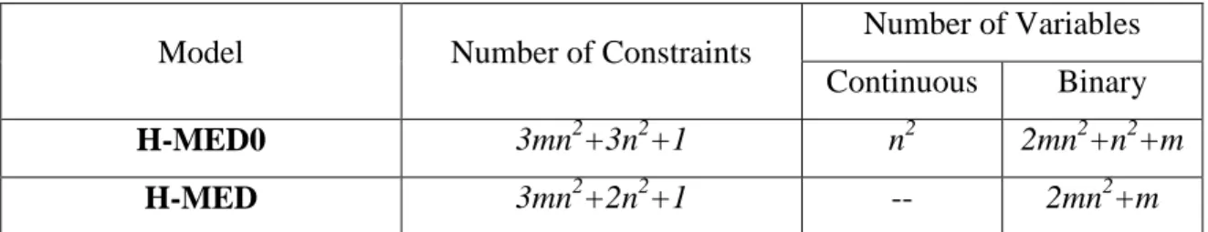
We can easily argue that H-MED correctly linearizes the (r|Xp) hub-medianoid problem with fewer variables and constraints than H-MED0. The following table depicts the number of variables and constraints of both models where n is the number of nodes and

m is the number of available nodes to locate hub in the network, that is |N| = n and |H| = m.

Table 4-1: Comparison of H-MED0 and H-MED in terms of size of the models

Model Number of Constraints Number of Variables

Continuous Binary

H-MED0 3mn2+3n2+1 n2 2mn2+n2+m

H-MED 3mn2+2n2+1 -- 2mn2+m

4.2 Problem Complexity

We prove that the problem of finding a (r|Xp) hub-medianoid is NP-hard and the corresponding decision problem is NP by using reduction from clique problem, an NP-complete problem by Karp [56].

Decision Version of Clique Problem: Given an undirected graph G=(N,E) and an integer r, determine if G has a r-clique, that is, there is a set of vertices K with |K| ≥ r such that for each pair of vertices in K there is an edge in E between them.

Theorem 1: (r|Xp) hub-medianoid is NP-complete even if α = 0.

Proof: (r|Xp) hub-medianoid problem is clearly in NP since given the set of leaders and followers hubs for each pair of nodes i,j ∈ N, we can solve the shortest path problem and determine if the flow wij is captured or not. This process can be done in polynomial time. Given an instance of clique problem, we construct a network G’=(N’,E’) where N’ = N U Xp, where Xp = {x1,x2,...,xp} and E’ = E U {(i,j): i ∈ N and j ∈ Xp} where Xp is

(42)

32

assumed to be the hub set of the leader. Let cij = 1 if (i,j) ∈ E and cij = 0.5 if i ∈ N and j ∈

Xp and let α = 0. The flow values for all pairs i,j ∈ N is set to 1. Clearly βij = 1 for all i,j ∈ N.

We prove the theorem by showing that there exists a set of r points Yr(Xp) on G’ such that ( ) ≥ C(r,2) = (r2

-r)/2 if and only if there exists an r-clique on G where C(r,2) is 2-combination of a set with cardinality r.

Assume that clique problem has solution K ⊆ N and |K| ≥ r. By letting Yr ⊇ K, we can observe that γij = 0 for all i,j ∈ K since all flows on the clique benefit discounting where

α = 0 and the total flow among the clique is captured by the follower, that is,

( ) ≥ (r2

-r)/2.

On the other hand, suppose Yr in G’ is such that ( ) ≥ (r2-r)/2. If for all i,j ∈

Yr there exists an edge (i,j) ∈ E, then Yr itself form an r-clique on G. Then set K = Yr. Otherwise, assume that Yr does not form an r-clique, then there must be (r2-r)/2 units of flow captured by the follower and at least one unit of flow should be routed via a spoke link. Equivalently, we can say that for (r2-r)/2 pairs of node γij < 1. Then, none of the captured flow is routed via spoke link of the follower which contradicts with the assumption.

Hence, we conclude that (r|Xp) hub-medianoid is reducible from clique problem in polynomial time. So, it is NP-hard. □

4.3 Computational Study

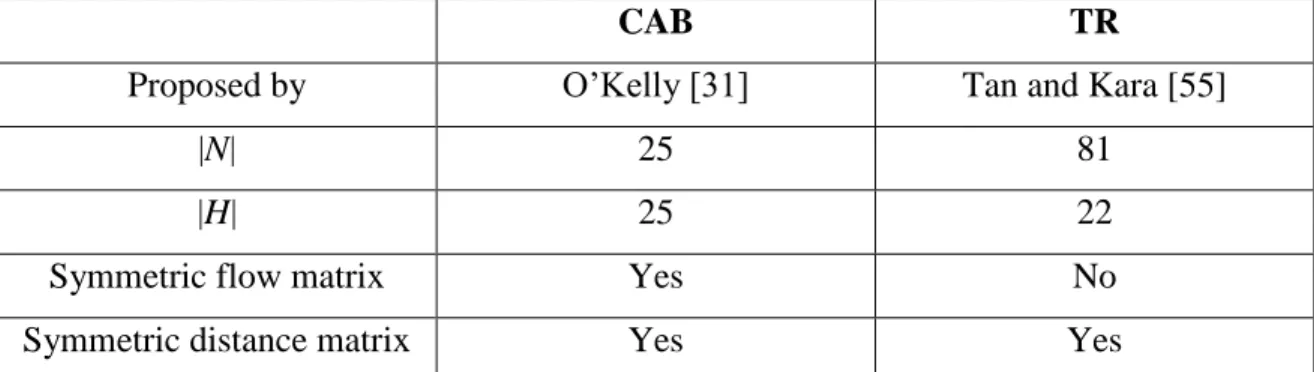
Performance of H-MED is investigated by the computational experiments conducted on two different data sets: CAB and TR. The following table summarizes properties of CAB and TR data sets.

(43)

33

Table 4-2: Summary of properties of CAB and TR data sets

CAB TR

Proposed by O’Kelly [31] Tan and Kara [55]

|N| 25 81

|H| 25 22

Symmetric flow matrix Yes No

Symmetric distance matrix Yes Yes

values are chosen as either or . Also, for TR data set results for are obtained since Tan and Kara propose that this value is obtained from cargo companies of Turkey [55]. Nodes in the CAB data set are numbered based on the alphabetical order of the city names whereas nodes in the TR data sets are plate codes of cities in Turkey which ranges from 1 to 81. The maps showing the spatial locations of nodes and potential hubs of CAB and TR data sets can be found in Appendix 1 and 2, respectively. All instances are solved with CPLEX 12.4.0.0 and a 4 x AMD Opteron Interlagos 16C 6282SE 2.6G 16M 6400MT computer running under Linux operating system.

Since we need to take βij values as parameters of (r|Xp) hub-medianoid problem, we have to make some assumptions for the leader’s hub set in advance. Therefore, we consider that the leader locates his/her hubs on a set of nodes according to his/her optimal choices of well-studied multi-allocation hub location problems: uncapacitated

multi-allocation p-hub median (UMApHM) and p-hub center (UMApHC). However,

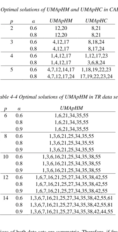
current models in the literature are not able to solve the UMApHC for the size of TR data set, so only UMApHM solutions are used as leader’s hub set for this data set. Table 4-3 and 4-4 show the optimal solutions of UMApHM and UMApHC problems that are used in the computational study.

(44)

34

Table 4-3:Optimal solutions of UMApHM and UMApHC in CAB data set

p α UMApHM UMApHC 2 0.6 12,20 8,21 0.8 12,20 8,21 3 0.6 4,12,17 8,18,24 0.8 4,12,17 8,17,24 4 0.6 1,4,12,17 1,12,17,23 0.8 1,4,12,17 3,6,8,24 5 0.6 4,7,12,14,17 1,18,19,22,23 0.8 4,7,12,17,24 17,19,22,23,24

Table 4-4 Optimal solutions of UMApHM in TR data set

p α UMApHM 6 0.6 1,6,21,34,35,55 0.8 1,6,21,34,35,55 0.9 1,6,21,34,35,55 8 0.6 1,3,6,21,25,34,35,55 0.8 1,3,6,21,25,34,35,55 0.9 1,3,6,21,25,34,35,55 10 0.6 1,3,6,16,21,25,34,35,38,55 0.8 1,3,6,16,21,25,34,35,38,55 0.9 1,3,6,16,21,25,34,35,38,55 12 0.6 1,6,7,16,21,25,27,34,35,38,42,55 0.8 1,6,7,16,21,25,27,34,35,38,42,55 0.9 1,6,7,16,21,25,27,34,35,38,42,55 14 0.6 1,3,6,7,16,21,25,27,34,35,38,42,55,61 0.8 1,3,6,7,16,21,25,27,34,35,38,42,55,81 0.9 1,3,6,7,16,21,25,27,34,35,38,42,44,55

The distance matrices of both data sets are symmetric. Therefore, if from node i to node

j is routed via the leader’s (follower’s) hubs then flow from node j to node i is also

(45)

35

and (4.12)-(4.15) of H-MED are imposed for only i < j and the objective (4.11) is replaced with ∑∑ for computational studies.

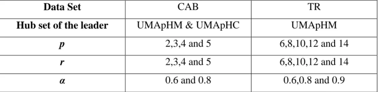
The following table summarizes all of the totaling up to 139 instances used in the computational study of (r|Xp) hub-medianoid problem:

Table 4-5: Summary of the instances used in the computational study

Data Set CAB TR

Hub set of the leader UMApHM & UMApHC UMApHM

p 2,3,4 and 5 6,8,10,12 and 14

r 2,3,4 and 5 6,8,10,12 and 14

α 0.6 and 0.8 0.6,0.8 and 0.9

Table 4-6 summarizes the CPU time, the market share and hub sets of the follower in the optimal solution of (r|Xp) hub-medianoid problem where the follower has already located his/her hubs on the optimum solution of UMApHM and UMApHC on CAB data set with α = 0.6.

(46)

36

Table 4-6: Results of the (r|Xp) hub-medianoid problem on CAB where Xp = UMApHM

with α = 0.6 p Leader's hubs = UMApHM r = 2 r = 3 r = 4 r = 5 2 {12,20} CPU 6.15 5.59 7.95 12.49 Share 65.62% 78.25% 87.08% 92.26% Hubs {2,6} {2,6,12} {2,6,12,19} {2,5,12,19,20} 3 {4,12,17} CPU 11.16 9.05 14.15 10.97 Share 30.49% 45.13% 53.69% 62.02% Hubs {17,25} {17,21,25} {9,17,18,21} {9,17,18,21,22} 4 {1,4,12,17} CPU 23.44 17.93 20.79 24.61 Share 17.91% 28.39% 37.73% 46.18% Hubs {2,21} {17,21,25} {14,17,18,21} {9,14,17,18,21} 5 {4,7,12,14,17} CPU 11.28 9.32 12.63 10.55 Share 18.64% 28.14% 35.04% 42.32% Hubs {17,25} {9,17,18} {9,17,18,21} {9,17,18,21,22} p Leader's hubs = UMApHC r = 2 r = 3 r = 4 r = 5 2 {8,21} CPU 2.86 4.32 4.74 3.69 Share 75.86% 85.20% 90.98% 94.74% Hubs {5,19} {4,13,19} {4,8,12,13} {4,8,12,13,21} 3 {8,18,24} CPU 6.45 4.63 15.68 18.3 Share 51.81% 70.25% 79.08% 85.23% Hubs {4,17} {5,17,19} {5,14,17,19} {6,14,17,19,21} 4 {1,12,17,23} CPU 21.72 22.67 20.94 19.91 Share 36.56% 47.39% 57.38% 66.93% Hubs {18,20} {18,20,24} {13,18,20,24} {13,18,19,20,24} 5 {1,18,19,22,23} CPU 6.75 13.39 16.08 10.96 Share 45.62% 57.27% 69.34% 76.75% Hubs {4,17} {1,5,17} {1,5,12,17} {6,12,13,17,24}

Since the leader chooses his/her hub locations without being aware of competition, the follower can capture high amounts of flow even p = r. For example, if p = r = 2 the follower can capture more than 65% of total demand.

The proposed mathematical model H-MED can be regarded as the formulation of