Щ;· - ,
...- .■
___
ICE DEPEÑ!
IT ■
CT*'$ ;T--4»r*4!S
PRICE DEPENDENT PROCUREMENT DECISIONS IN
ONE-PERIOD INVENTORY PROBLEM
A THESIS
SUBMITTED TO THE DEPARTMENT OF INDUSTRIAL ENGINEERING AND THE INSTITUTE OF ENGINEERING AND SCIENCES
OF BILKENT UNIVERSITY
IN PARTIAL FULFILLMENT OF THE REQUIREMENTS
FOR THE DEGREE OF MASTER OF SCIENCE
By
Hakan Polatoglu June, 1989
t S
( bo
P
I
I certify that I have read this thesis and that in my opinion it is fully adequate, in scope and in quality, as a thesis for the degree of Master of Science.
Ш Ж и и ^ .
Prof, izzet Şahin(Principal Advisor)I certify that I have read this thesis and that in my opinion it is fully adequate, in scope and in quality, as a thesis for the degree of Master of Science.
. Prof. Nesim Erkip
I certify that I have read this thesis and that in my opinion it is fully adequate, in scope and in quality, as a thesis for the degree of Master o f Science.
Asst. Pr<if. Cemal Dinçer
I certify that I have read this thesis and that in my opinion it is fully adequate, in scope and in quality, as a thesis for the degree o f Master of Science.
Asst. Prof. Levent Onur
Approved for the Institute of Engineering and Sciences:
Prof. Mehmet Bara
ABSTRACT
P R IC E D E P E N D E N T P R O C U R E M E N T D EC ISIO N S IN O N E -P E R IO D IN V E N T O R Y P R O B L E M
Hakan Polatoğlu
1^1.S. in Industrial Engineering Supervisor: Prof. İzzet Şahin
June, 1989
In this work the classical newsboy model is extended by introducing a price dependent demand pattern. It is intended to obtain optimal procurement and pricing decisions for maximizing the expected profit. It is shown that, both decisions can be made simultaneously if we are able to identify the effects o f price on the demand process.
ÖZET
Т Е К d ö n e m l i e n v a n t e r p r o b l e m i n d e f i y a t a B A Ğ L I ENIYI T E D A R İK M İK T A R I
Hakan Polatoğlu
Endüstri Mühendisliği Bölümü Yüksek Lisans Tez Yöneticisi: Prof, izzet Şahin
Haziran, 1989
Tek dönemli klasik envanter probleminde beklenen eniyi kârı veren tedarik miktarı bu lunurken malın satış fiyatı sabit olarak alınmaktadır. Ancak, ideal olmayan pazar şartlarında istem ile fiyat arasındaki ilişki göz önüne alındığında stok miktarının fiyattan etkilenebileceği düşünülmektedir. Bu çalışmada, en büyük kâr değerini veren stok ve fiyat kararları yukarıdaki fikirden hareket ederek eşzamanlı olarak bulunmuştur. Çözülen sayısal örnekler ve kuramsal sonuçlar göstermektedir ki, stok miktarına ek olarak verilecek fiyat kararı probleme yeni bir yönetsel boyut getirebilmektedir.
ACKNOWLEDGEMENT
The author welcomes this opportunity to express his gratitude to Professor İzzet Şahin for his supervision o f this thesis and his continual interest. lie is also indebted to the members o f his thesis committee: Associate Professor Nesim Erkip, Assistant Professor Cemal Dinçer, and Assistant Professor Levent Onur for their advice and support.
A special note o f thanks is due to Associate Professor Ömer Benli, on behalf o f the Bilkent University Industrial Engineering Department for providing an excellent research environment for the entire study.
Contents
1 IN T R O D U C T IO N A N D LIT E R A T U R E R E V IE W
i
2 BASIC PR O B LEM A N D A S S U M P T IO N S
3
3 M ATH EM A TICA L M O D EL
6
3.1 General Expected Profit Function... g
3.2 Expected Profit Function With Constant Unit C o s t s ... g
3.3 Mathematical Programming Formulation and General Solution Procedure . .
7
3.4 Certainty P ro fit...
3
3.5 Additional Set-Up C o s t ... 20 4 EX A M PL E S17
4.1 Example1
... 27 4.2 Example 2 ... 24 4.3 Example 3 ... 28 5 SU M M A R Y A N D C O N C L U SIO N S 30 VllCONTENTS
A P P E N D I C E S
Api)endix A
A p p en d ix B
A p p en d ix C
A p pendix D
A p p en d ix E
Vlll 31 32 36 37 3 9List of Figures
2.1
Physical Model of the One-Period Problem...3
3.1
Construction OfI4
3.2 7l/(u,pu) Function... jg
4.1 The Cross-Hatched Area Represents the Price-Demand Values That Can be Realized Under the Assumptions (
4
.2
) and (4
.3
) ...4.2 The Cross-Hatched Area Represents the Price-Demand Values That Can be Realized Under the Assumptions (4.2) and (4 .1 4 )... 24
B .l The Definition of 0 (w ,p )...
33
B.2 A General 0 (u ,p ) Function in w...
34
List of Tables
4.1 Results o f Example
-1
...2
i4.2 Results of Example-1...
22
4.3 Results of Lau L· Lau... 23
4.4 Results of Example-2... 26
4.5 Results o f Example-2... 27
Chapter 1
IN T R O D U C T IO N A N D
LITERATUR E R E V IE W
The literature on inventory systems abounds with studies that address the question of how much inventory to hold and how. In almost all of these studies the product selling price is taken to be an exogeneous variable. There is a need to incorporate the pricing issue into the decision problem, however, to achieve an increased level of economic soundness in modelling.
The price-demand relation is one o f the fundamental concepts of the theory of the firm
in the neoclassical economic theory. TYaditionally, this relation was studied under economic equilibrium where the demand becomes deterministic once the price is given. Later (see [
2
,3,5,6
,7,9] ), uncertainty was introduced into the problem where demand to be realized at any price level was taken to be random.A number o f researchers have been interested in the pricing concept as it relates to inventory theory (e.g., [3,10,12,13,14,15,16,17,18,19,20,21,22,23,24,25]). Few among those, however, were interested in the price-demand interaction. Most of them studied the effects of various procurement or selling price adjustment scenarios on the EOQ formulation. Since the amount of inventory to be held is strongly dependent on demand distribution, which in turn is affected by the product price, there is a need to determine the best procurement quantity and pricing decisions simultaneously.
To discuss the price-demand relationship, the structure o f the market should be identified first. In perfect competition the market price is determined by various equilibria present in the economic system; the atomistic firm is a price taker. For such a firm it remains to make output decisions in view of expected rises and falls in the market price and demand. Hence, given the optimal output decision, the price will be determined by market equilibrium which is assumed to be reached instantaneously. On the other hand, in imperfect competition the firm can set the product price. However, the demand to be realized at a given price level
CHAPTER 1. INTRODUCTION AND LITERATURE REVIEW
is uncertain. Naturally, the firms should undertake a forecasting effort in order to have an idea about the characteristic price-demand relationship of the market.
In his pioneering work, Mills [3] studied short-term output and pricing decisions of a firm producing a single product and facing imperfect competition. For maximizing the expected profit objective, he showed that, in the case of demand uncertainty the optimal strategy differs from the deterministic case. Baron [
6
] elaborated on the same subject releasing more structural results. Sandmo [7] and Baron [5] studied the same problem by introducing the idea of risk. In their models the utility (cf. Von Neumann and Morgenstern [1
]) of the expected profit is maximized. They showed that pricing and output decisions are affected by the risk attitude o f the firm. Leland [9] contributed to the subject by generalizing the problem for three cases, namely, the quantity-setting firm, the price-setting firm, and the price- and quantity-setting firm. For the risk-neutral case the results o f the above studies have implications on the pricing issues related to the one-period inventory problem.In a recent paper, Lau L· Lau [22] attacked the pricing issues related to the one-period inventory problem. They showed how the pricing decision can be studied as a new problem in addition to the procurement decision. For maximizing the expected profit, they indicated that there exists no analytical solution for the optimal price value for a general demand distribution. Instead, they proposed a numerical solution procedure. Their results will be referred to in the sequel.
Abad [25] studied the joint price and lot-size determination problem for a multi-period inventory system facing deterministic demand. In his work, demand is expressed as a function of price. He solves the tradeoff between low price high demand and high price low demand under certainty. We shall study this deterministic situation for one-period problem in detail in section 3.4.
Gerchak and Parlar [20] approached to the one-period problem from a different view point. They considered a random potential market size. The firm captures a certain percentage of this allowable potential due to its sales effort. Therefore, under a constant market price there exists a tradeoff between high sales effort high demand and low sales effort low demand. Although, in this problem they have no pricing decision the main idea is to alter the demand distribution by a decision variable, which is similar to our bcisic understanding.
We close this section by noting that, in this study we assume that the decision maker has a neutral risk attitude. Hence, his objective is to maximize his expected wealth (profit). The idea o f risk is, therefore, beyond the scope of this work. Interested reader can refer to [
11
] for more information.BASIC PROBLEM A N D
ASSU M PTIO N S
Chapter 2
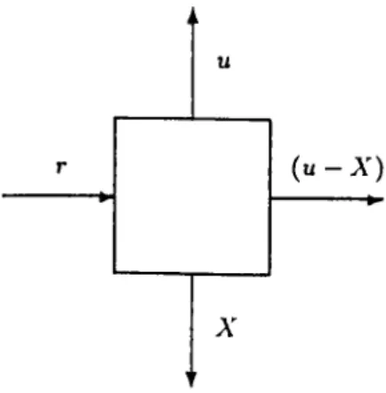
The physical model of the one-period problem is depicted in Figure-2.1. The economic model is built on this physical system with the following considerations and assumptions :
u
r ( u - X )
X ’
Figure 2.1: Physical Model o f the One-Period Problem where
r
u X
( u - X )
initial inventory level (r >
0
), beginning inventory level,random demand with p.d.f. o f /( · ) , leftovers if ti > A", or shortages if u < A'.
(A l): The order quantity is (w - r) but, u is taken to be the decision variable where v > r, and there is no capacity limit on u.
CHAPTER 2. BASIC PROBLEM AND ASSUMPTIONS
(A2): The costs associated with tlie problem are expressed in the following functional forms:
Procurement Cost = C(u — r) if u — r > 0
0
if li — r <0
Shortage Cost = S{ X - u) if X - u >
0
0
if A' — li <0
Holding Cost H { u - X ) i f u - X > 0
0
if u - X <0
where C( ),5 (·), and ) are positive valued functions. Note that we can incorporate the salvage value into the function H{ ).
(A3): We assume that the vendor is in imperfect competition. That is, he can set any price between Pt and P^ {Pi >
0
), where Pt is the lower bound and P^ is the upper bound on the product price that are induced by economic conditions or set exogeneously. We also assume that demand can be realized at any price between Pi and P^.(A4): The vendor is certain on forecast results; that is, he believes the forecasters 100 %.
(A5): In general, the quantity demanded (A^) and the price level (p) are dependent through the following implicit function
jr ( X ,p ,c ) =
0
(2
.1
)where £: is a random variable. [9] . Therefore, we can solve for X
A' = X ( p ,f )
in terms o f p and e. Furthermore, we can assume that the random term is additively separable in the form :
A^ = A » + £(p) (
2
.2
)where X (p ) is the expected demand at the price level o f p. Equation (2.2) makes sense because, e{p) becomes the forecast error term which is added to the mean regression curve X (p ) to yield the random demand. In his work. Mills [3] further assumes that the forecast error term is independent o f p. That is, the forecast is equally predictive at any price level. In this study, we shall consider a more general relation given by (2.2). Lau L· Lau [22] also consider a similar relation to (2.2).
(A
6
): Expected value o f the quantity demanded at the price level of p is expressed as X (p) which is a continuous and differentiable function o f p. We assume that X (p ) is a monotone decreasing function; i.e.,dX{p) dp
< 0
CHAPTER 2. BASIC PROBLEM AND ASSUMPTIONS
(A7): The forecast error e{p) is assumed to be a continuous random variable with a p.d.f. of
g{x;p) i ^i(p) < X < ^2(p)> and zero mean for all p G [PiyPu] ‘
J
r^2(p)f x-g(x-,p)-dx =
0
, ti(p)where €i(p) and £2{p) > being continuous functions of p , are the bounds on £:(p), if they exist, and p is a parameter o f g{']p). Also, we assume that g{x;p) is a unimodal p.d.f. and is differentiable in p and x. Consequently, the c.d.f. of the forecast error,
G{x'iP)=
f
g{i\p) dt ,becomes continuous and differentiable in both x and p , and monotone increasing in x.
(A
8
): From (A5) and (A7) the demand distribution can be obtained as<;(x - A '(p);p) , Clip) + A (p ) < x < £T
2
(p) + A (p ),f{x',P) =
and the c.d.f. of demand becomes
otherwise, /•X AX-X(p) P' (x, P)= / f{t\p) d t - / g{ y\p) - dy=G{ x - X{p)\p). Note that E[X;p] = jf fa(p)+*^(p) rra(p) t f ( t ; p ) d t = / [y + A ( p ) ] i ( p ; p ) < / j / = A (p ). 7 i,( (p)+^(p) i(p)
It became a common practice in the field to use a normal (or any other Pearson type) distribution to represent the demand process. This practice however, is only an approxima tion because demand can never be negative or infinite in reality. The approximation is based on the negligable probability of occurrences of very large or negative values. In this study we will prefer to work with a non-negative and finite demand process. Therefore, we require that the limits o f the demand distribution are positive and finite at all feasible price levels. That is:
Chapter 3
M A T H E M A T IC A L M O D EL
3.1
General Expected Profit Function
Under the assumptions, profit П(р, u) of the vendor becomes
n (p „ ) = / P· ^ - - »·) - ^i(p) + ^(P) <
I p u — C{u — r) — S{ X — u) , if a < A”" < £
2
(p) + A (p ).Using (A
8
) the expected profit can be obtained fromj? [n (p ,u )]=
f
\p x - C { u - r ) - H { u - x)] fix\p) dxЛ,(р)+А'(р)
j(p)+-^(p)
+ / \p-u - C{u - r) - S(x - u)]-f{x\p)-dx. Ju
(3.1)
3.2
Expected Profit Function W ith Constant Unit Costs
To facilitate the mathematical analysis, general expressions in (A2) will be simplified as follows:
C(a:)
= C'X
S{x) = s x ^ (3.2)
H{x) = h x
where
c,s,
and h are constant unit costs given in $/unit. Note that no fixed cost terms are allowed in (3.2). The case of additional fixed procurement cost will be considered later. Using (3.2) in (3.1) we writeCHAPTER 3. MATHEMATICAL MODEL
E[U{p,u)] P‘X(p) - c-(ii - r) - h· { u - x ) ‘f { x ; p) dx
r€2(p)+X(p)
- ( p + « ) · / (x - u)- f{x; p) dx. J U
Using (A
8
) and substituting y = x — X{p) in (3.3) we obtainJE:[n(p,ii)] = p X { p ) - c { u - r ) - h · W - X ( p ) - y ] - g ( y \ p ) dy Jci(p) r^2(p) - ( ? + « ) · / [ y - w + .A'(p)] ff(y;p)-dy. Ju- X( p) Rewriting (3.4) we get £'[n(j>,ii)] = c-r + ( p + 5 - c) ii - 5-X(p) - (p -f S + h) Q{u, p), where l^u-X(p) _ I^u-X(p) 0 ( « . P ) = / W - ^ ( p ) - y ] - 9 i y , p ) d y = G{y\p)dy. Jti{p) dei(p) (3.3) (3.4) (3.5) (3.6)
For details o f the derivation of equation (3.5) see Appendix-A. The function 0 (w ,p) is studied in Appendix-B.
3.3
Mathematical Programming Formulation and Gen
eral Solution Procedure
The objective o f the vendor is to maximize f[IT(p, u)] by making the best procurement and price decisions.
The problem can be formulated as a nonlinear optimization problem as
iT [n(p·, u·)] = Max { £ ’[n(p, u)] : (p, w) G 3^} p,u
(3.7)
s.i. y = {(p, u) : r < u < oo , Pi < p < Pu) ·
Since £'[n(p, u)] is continuous in u and p, it has a global maximum over 3^. By assumption (A
6
), A'(p) is differentiable in p and from Appendix-B it follow^s that 0 (u ,p ) is differentiable in both u and p. Therefore, £'[II(p, n)] becomes differentiable over 3^ so that the first and second order optimality conditions can be studied by taking partial derivatives. However, since the expressions in the hessian becomes impractical for a clear analytical study, w’e shall prefer an alternative approach.CHAPTER 3. MATHEMATICAL MODEL Considering (3.5), we write дЕ[П(р,и)] ди д^ЕЩр,и)] ди^ = { p + s - c ) - { p + s + h) G{u - Х (рУ,р), = - i P + s + h ) g ( u - X ( p ) ] p ) < 0 . (3.8) (3.9)
which immediately proves that for any p , £'[n(p, i/)] is concave in u. Therefore, the optimal procurement decision u* can be obtained from the following as a function of p
(0 G (« ’ - A 4p) ;p) = ^ — f = 1
-p - f s - h / i p - f s - f / ?
(ii) if u* < Г then set u* = r.
(3.10)
It is essential to note that, we obtain a unique solution for (3.10) for any price value between zero and infinity, if it exists.
Again from (3.5) we obtain
(3.11)
It is evident from (3.11) and (3.12) that for the general case it may not be trivial to solve for p* which maximizes £ ’[П(и,р)] for a given u. For a special problem, however, we can solve for u* in (3.10) as a function o f p and substitute it in (3.5). Then, through a functional analysis over p we can evaluate the global maximizer p*. We shall illustrate the use o f this method in the example problems.
3.4
Certainty Profit
If there is no uncertainty, then we have e = 0 with probability one and the demand becomes deterministic at any price level. In this case we write the certainty profit as
Пс(р,іі) = p ti - c (w - r) - S'[A (p) — ti] , if w < ^{p)^
p-JV(p)
- c (ti - r) - /i [u -A(p)]
, if ti >A'(p).
Therefore, we obtain the optimal decisions fromΠ c(p ^ t^ ;)= Max {П с(р ,и ): г < u < oo , Р / < p < Pti).
Given p, suppose u < X{p). Then we have
n<:(p, u) = (p + s - c)-u - s-X{p) + c r. (3.14)
Since, (3.14) is a linear increasing function of u, we get «* = X{p). Therefore, we write
n c(p ,u j) = ( p - c ) . A '’(p) + c-r. (3.1.5)
CHAPTER 3. MATHEMATICAL MODEL
9
Now, suppose и > X{p). Then we have
Пс(р, = (p-l· h) X{p) - + h) -f c r (3.16)
which is a linear decreasing function of u. Therefore, u* becomes the smallest possible u
which is given by:
"(p ) , if A (p ) > r, , i f A '( p ) < r . Consequently, we write (3.17) П с ( р , < ) = | (p - c) A (p ) + c.r , if A (p ) > r, (p + Л)-А(р) - Л-Г , i f A ( p ) < r . (3.18) Let Pi be defined by A4Pi) = r,
such that Pi G [Pi, Pu]· If г < X{Pu) then set pi = Pu, and if r > A"(P/) then set pi = Pi.
If P ^ Pi then, A (p ) < A (Pi) = r. We can not have и < A (p ) < r. Therefore, we only consider the case o f u > -Y(p). From (3.17) and (3.18) we get
n c(p ,ti:) = ( p + A ) A ( p ) - / i . r , (3.19)
and u* = r.
If p < Pi then, A"(p) > A (p i) = r. We can have either u > X(p) or u < A’ (p). However, in either case, from (3.15) and (3.18) we get
П с(р ,«:) = ( p - c) A (p ) + c r,
and ti* = A (p ). Therefore, from (3.19) and (3.20) we obtain
( р + Л ) А ( р )
-П с(р,
0
= < . ,(p -c )..\ t p ; + c r ,
u; = X(p).
Problem (3.13) can be rewritten in the following form
(3.20) > ) - h r, ) < = r. / ’for p > Pi, (3.21) , for p < P i. Пс(р: ,и: ) = Max {П с(р ,и * ): Pt < p < Pu) P (3.22)
CHAPTER 3. MATHEMATICAL MODEL
10
where IIc(p, w*) is given by (3.21). Since X{p) is continuous by assumption (A
7
), Ilc(p, u*) is also continuous; hence, it has a global maximum over [Pi, P^], say at p*.Note that for r = 0 we have p < pi, and from (3.21) we get u* = A”(p), and
n e (p ,«* ) = ( p - c ) A '( p ) . (3.23)
The idea o f comparing the uncertainty and certainty results was introduced by Mills [3]. This enables us to see the change in the expected profit and decision variables due to the uncertainty introduced into the problem. We shall provide this comparison for the example problems.
3.5
Additional Set-Up Cost
In this case we allow for an additional (constant) term fC in the procurement cost function
C(a(a;) = <\ fC + c x , if
\
0
, ifa: >
0
, a; =0
.Therefore, the profit function becomes
„ , ^ ( p x — K — c (u — r) — h-(u — X
n / ( p , « ) = < t- ( \ Í
I p u — fC — c (u ~ r) — S'(x — u
- x )
,
fi(p) + A'’(p) < a: < u,
) , u < x < ^ 2 Í p ) + X(p),and we can write the expected profit as
EUlfip
where L{v,p) is the expected loss function given by :
- r) - I ( u , p ) + p A'(p) , if u > r , p X{ p) , if « = r, (3.24) I ( u ,p ) = h - [ { u - x ) f{x; p)-dx Jei(p)+X{p) (3.25) f (p + s)· / Ju f3(r)+A(p) { x - v ) f { x \ p ) d x ,
= (p + s) [A'(p) - ti] + ( p + s + /i)-©(w ,p).
See Appendix-C for the derivation o f (3.26).
Furthermore, defining a function ^í{u,p) as :
i l/( « ,p ) = L(u,p) + c {u - r ) - p X{p),
(3.26)
CHAPTER 3. MATHEMATICAL MODEL 1 1 -£ [n y (p ,«)] = \ M(r,i we can write ,p) + K. , if V > r, ,p) , if u = r. Note that M(u,p) = - ^ [ n i p .u ) ] .
In this regard, the optimization problem becomes
~-E[Uj(p%u^)]= Min { - i : [ n ; ( p , i / ) ] : ( p , i i ) G y }
p,u
s.i. y ^ {{p,u) : r < u < oo , P t < P < P u } ·
(3.28)
(3.29)
Since jE'[IT/(p, u)] is discontinuous at u = r, we need a different analysis than we have developed for (3.7).
For the classical newsboy problem with a constant set-up cost we define the optimal policy by two parameters namely, the reorder point (s) and the order-up-to level (S). This is known as the {s,S) policy. For our model the presence o f an {s^S) type policy is an important fact because, it might have useful implications for the multi-period extension of the theory. In this regard, we shall reveal the conditions under which an (s,5) type policy would yield the optimal decisions.
o ®
Let u and p^ be given by the relaxed problem
/ o ®
A f(w ,P u )= -A/in {M (u ,p ) :
0
< u < oo , P t < p < P u ] >XI,p (3.30)
/0 ^
Since M{u, p) is continuous in p and u, there exists a solution {u,p^^) for the problem (3.30). This problem can be rewritten as:
,0 o
M{ u, Pu) = Min { M{ u, pu) : 0 < u < o o } ,
u
where pu is the best price value at u and it can be determined from
M (u ,p u )= -A/m { M{ u , p ) : P e < P < P u ] ‘ P
(3.31)
(3.32)
We claim that, we can device an (s,S) type policy which will operate on M (u,Pu) ,and we can utilize that to obtain the optimal decisions. This requires M{u,pu) to be A^-convex in ti. We shall prove our claim but, before getting into details o f the proof we need to study
M(u,pu) further.
CHAPTER 3. MATHEMATICAL MODEL 1 2 M (u ,p ) =
1
s*A"(p) — -f s — c) — c-r 5-.Y(p) - + s - c) - c-r + (pH-5
-f /i)-0 (w ,p ) -(p H -/i)-.V (p ) H - / i ) - c- r , £Ti(p) H- JV(p) > u > 0, , otherwise, , S2{p)-\-X{p) < u. (3.33)In this representation, M{ u, p) becomes a monotone decreasing function o f p for u < ¿:i(p)H- A"(p). Therefore, for 0 < u < Ci{Pu) H- X{Pu) we have Pu = Pu and
X^(^iPu)
= <S-A'(Pu) —U’{Pu
H- 5 - c) — c-r (3.3H) which is a linear (decreasing) function o f u with a slope o f —(P^ H-s —c). We call this function as the left tail of M{UjPu)>If, on the other hand, u > e^ip) H- X{p) then we have
M{u,p) = -(p H - h)^X{p) H- m (cH- h) - c r. (3.35)
For any li, the price which minimizes (3.35), say pu, can either be a boundary value, or an interior value. If former then, pu = P/, or p„ = Pu · M{u,pu) becomes a linear function of
u. If latter then, pu is a relative minimum point which should satisfy
dM{u,p^) _ - (-n I M
---—--- = 0 = - A ( P u ) - ( P u + /l)— — — .
OPu OPu (3.36)
Note that the condition (3.36) is independent of t/, hence, for all u > S2{p) H- A'(p) we have a unique Pu, if it exists.
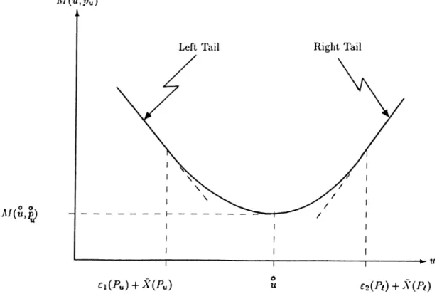
Therefore, for u > €2{Pi) X( Pi ) we have a unique pu. In this range, M (u,pu) becomes a linear (increasing) function of u with a slope o f (cH- h). We call this linear function as the right tail o f M (u ,py).
We can therefore, interpret the right and left tails o f M{u,pu) as its “asymptotes” in a sense that above the maximum and below the minimum beginning inventory levels the function is linear (convex) in u.
We also note that, the first and third form of M{u,pu) in equation (3.33) are equal to equations (3.14) and (3.16), respectively, with a sign change. This proves us that the right and left tails o f the function M (u,pu) become negative o f the certainty profit function in the appropriate u ranges.
When we solve problem (3.32) we get p^ either as a boundary value, that is, it becomes either Pi or Pu, or as an interior value. If there exists no interior point solution to (3.32) then the problem (3.31) becomes trivial. Therefore, we assume that there exists an interior point solution for some u.
CHAPTER 3. MATHEMATICAL MODEL
13
We already know that, if is a boundary value then M{u^p^) is convex in u. On the other hand, for interior point solutions we need to know the behaviour of A /(u,pu) in u.
If Pu € {Pi,Pu) then, it has to be a relative minimum point. Therefore, the best price at a given u has to satisfy
dM{u,pu)
dpu
=
0
.Writing the chain rule for differentiating M{u^pu) w.r.t. u as
dM{u,Pu) _ dM(v,pu) dM(n,pu) dpu
du du dpu du
and using (3.37) we obtain
dM(u,pu)
du = -{Pu + s - c ) + {pu + S + h ) G ( u - X(pu),Pu)·
(3.37)
(3.38)
We note that the first order condition on M{u,pu) yields
P u + s - c G{tl — X (Pu)i Pu) —
Pu + s + h ’ (3.39)
which implies that pu is the best price at u, and u is the best procurement at pu. Therefore, (3.39) gives the global minimum point (i/,Pu) for the problem (3.31). That is, every first order point o f M (u,pu) is a global minimum point o f (3.31).
It follows by (3.38) that,
dM(u,pu)
du < 0 <=> G{u - X{pu)\Pu) <
Pu -h g - c
Pu "l· s 4- (3.40)
Suppose that we choose a u, and obtain the best price at u as pu. Having p„ we now evaluate the best beginning inventory level tij from
(j (uj) A (pu ) J Pu ) —Pu + S - C Pu + s + /»
Since G{ ) is a monotone increasing function we write
(7 (u -A '(p u );p u ) < G («t - A'(pu);pu)
%i < U l .
Consequently, (3.40) becomes
dM(u,Pu)
CHAPTER 3. MATHEMATICAL MODEL U
P r o p o s it io n ;
M{u,Pu) is convex in u.
P r o o f b y c o n tr a d ic tio n ;
First we shall show that
dM{u,pu)
du < 0 , Vu G (0, u). (3.42)
Let
111
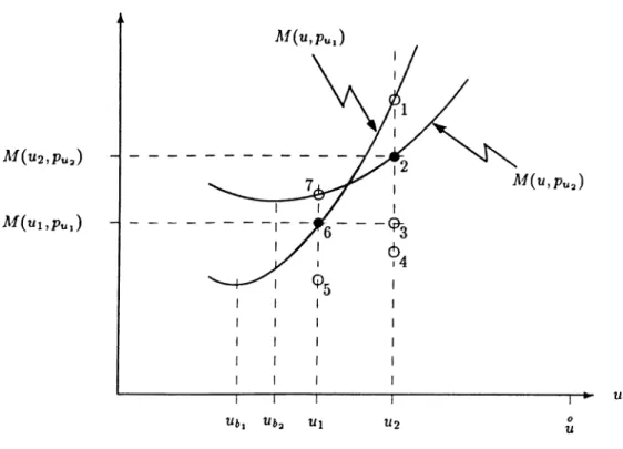
G (0 ,ii) and be the best price at tii. Suppose that we construct M (u ,pu i) in u and observe that it is increasing at ui therefore, the best procurement at say is less than ui. Furthermore, suppose that we move an infinitesimal amount to the right of ui, say to ii2
, and construct M(u,pua) where again < uo. See the proposed scheme in Figure-3.1.u
Figure 3.1: Construction O f M{v,p^).
We see in the figure that, when we make a pricing decision at ti
2
we can only reduce Tl/(ti2
,Pui) , that is, we can be at points 2, 3, or 4. Moreover, since M{u,p^^) is increasing at t/2
, it can pass through points 5 or 7. We have stated that point6
was the best price point at ui hence, M{u,pu^) can not pass through 5, because otherwise would have been better than p^^ at u\. Since point 7 is above6
,A/(u,pua) can not pass through 3 or 4.CHAPTER 3. MATHEMATICAL MODEL
15
Therefore, M{u,pu^) contains the points 7 and 2. It follows that, point 2 should be above point
6
and this behaviour reproduce itself every time we move to the right. When it happens that A/(u,Pua) contains points6
and 3 we say that it attains an extremum point in betweenui and U
2
. This, however can not be a relative minimum because, M{u,pu) can not rise to such a point. Thus, M(ujPu) increases until it reaches its right tail, which is described before.Concludingly, it becomes a contradiction to have u\, < u for any u G (
0
,u). Hence, we have ui > u and from (3.41) it follows thatdM{u,pu)
du
< 0
, V u G (0
,u).The same construction of the proof applies for u G (u, oo) where we have
dM{u,p^)
du > 0 (3.43)
by (3.38).
Consequently, by combining the results (3.42) and (3.43) we have M{u^p^) decreasing in u G (0,u ) and increasing in u G (u ,o o ). Thus, M{u,p^) becomes convex in u. A typical il/(u ,p u ) function is shown in Figure-3.2.
□
Now, suppose that we start with r units o f initial inventory, and do not procure anything. Then, the optimal pricing decision will be determined from
M(r,Pr) =
M { M
(r,p) : P/ < p < Pu}.P
(3.44)
Depending on the values o f r, 5, M (u, p,^), and M{r,Pr) the procurement decision, whether to order up to u or do not order, is made according to (3.28). It is clear with (3.28) that, whenever w’e place an order we incur a fixed cost o f K. Therefore, given an initial stock of r to start with, the optimal policy will be determined by the following (s,S) type procedure :
(j) Find M{u,Pu) and M (r,P r),
(ti) If u< r then, do not order and set p* =Pr, (ill) If u> r then, if M(u,p^) -f AC < M (r,P^) then
o ^
order up to u and set p* =Pu else,
o
do not order and set p* =Pr.
This procedure will be demonstrated for an example problem in the next chapter.
CHAPTER 3. MATHEMATICAL MODEL
16
M{u,pu)
M ( u , ^
Chapter 4
E XA M P LE S
We shall assume that, the expected value o f demand has a linear relation with price. That is,
X (p ) = a -
6
-p, (4
.1
)where a and b are non-negative parameters. The parameter b can be interpreted as the price sensitivity o f the expected demand.
Mills [3] studied the linear case as it is given by the equation (
4
.1
). Lau L· Lau [22], however, considered a slightly different equationA'(p) = a -
6
(4.2)where pm is the mid-price given by
Pm — "f A i ) / 2 .
In equation (4.2) we note that .Y(p) rotates about the point (pm,fl) for different b values, and with Pm = 0, equation (4.2) becomes (4.1). In this study we shall consider the case given by equation (
4
.2
).4.1
Example 1
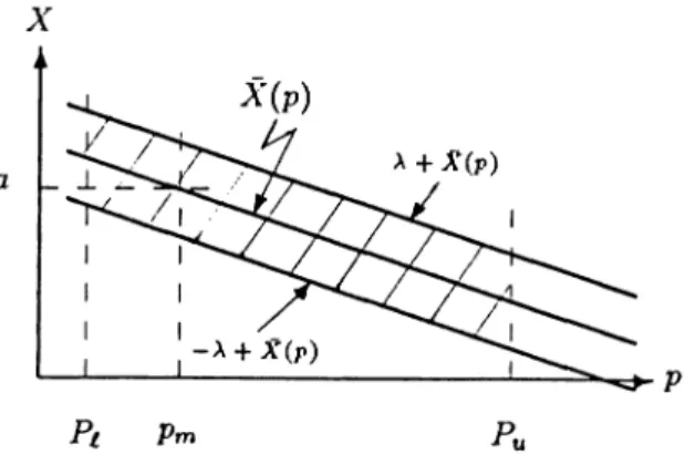
In this example we assume that the forecast error is independent o f the price and hcis a uniform p.d.f. given by 9i^,P) = //(a·) = 1 1 2A . - ^ < 2! < A, , otlierwise, (4.3)
where A > 0. Figure-4.1 displays possible price-demand realizations under conditions (
4
.2
) and (4.3).CHAPTER 4. EXAMPLES
18
A'
Figure 4.1: The Cross-Hatched Area Represents the Price-Demand Values That Can be Realized Under the Assumptions (4.2) and (4.3) .
Note that, the uniform distribution is not continuous at its limit points. Although, this contradicts with assumption (A7) we shall show that it is still possible to utilize the proposed method for obtaining the solution.
From (A7) it follows that
G(x) = ^
0
, X < —A, X -f A 2 A ’ - A < X < A,1
, A < X, (4.4)where the function becomes continuous in x, but not differentiable at i = —A, and x = A.
Taking r = 0 in (3.10) and using (4.4) it follows that
2 X { c + h ) « · = A (p ) I A -Furthermore, we evaluate
0
© ( « . P ) = · ! ¿^ • [w -A '(p )-f A]2
u - A '( p ) { p + s + h)' , for u < X(p) - A, , otherwise,, for u>A' (p)-fA,
(4.5)
(4.6)
from (3.6), which becomes a continuous functioii o f u and p. On substituting (4.6) in equa tion (3.5) with (4.5) we obtain
r [ n (;),u -)] = c r . f ( p - c ) A ( p ) - A ( c - f h) (p + s - c)
CHAPTER 4. EXAMPLES
19
which is a continuous and difTerentiable function o f p. Finally, using (
4
.7
), we get- A (p ) + (p c) ( p + , + , , ) ! ' (4.8)
y E [ n ( p ,» -) | ^ aX(p) d'-X(p) . i >. ( c + h f
dp^ dp (;>+5 + /l)3* (4.9)
Under the linearity assumption given by (4.2), and by utilizing (4.8) and (4.9), we employ a functional analysis to determine p*, the maximizer of (4.7). See Appendix-D for the details.
For the certainty profit, from (3.23) we write
^nc(p) dX(p)
- d T ~ + (4.10)
a=n,(p) „ dX(p) d^x(p)
(4.11)
Using (4.2) in (4.11) we find that Ile(p) is concave in p and from (4.10) we get
, _ o + b pm + b e Pc Moreover, we obtain 2-6 _ q + t pm - b e = î î± 1 b:l z± £ ) ! + , . , .
Table-4.1 displays the numerical results obtained for the following parameter set
c — 1,/i = 0.5, s = l , r = 0,a = 102, = 1.6, Pu = 4,p,„ = 2.8, A = 17.32,34.64,51.96,69.28,
b = 25,35,45,55.
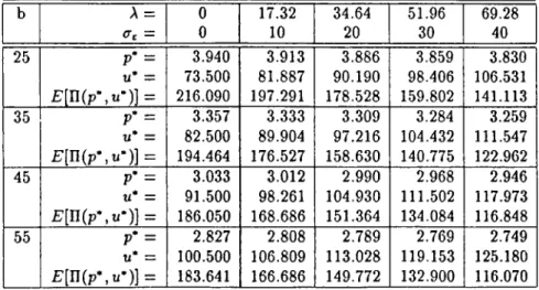
It is seen in Table-4.1 that as A (or standard deviation of the error term Cc) is increased, the optimal price declines slightly, the procurement quantity increases, and the expected profit decreases. It is intuitive to realize less profit as uncertainty in the problem increases, and order more in order to cope with uncertainties. Also, as b (i.e. the price sensitivity o f the expected demand) is increased the optimal price and the expected profit decrease but the procurement quantity keeps increasing. This result is intuitive too, because as price sensitivity increases the effect of uncertainties would also be coupled with it.
CHAPTER 4. EXAMPLES
19
which is a continuous and difTerentiable function o f p. Finally, using (4.7), we get
--- - A ( p ) + ( p - c ) . - g ^ - j ^ ^ - ^ ,
(4.8)^ ^ g [n (p ,» ·)] gJV(p) d^-X(p) 2 X ( c + h Y
5p2 dp 0p2 ■ ^ ( p + 5 + h)3· (4.9)
Under the linearity assumption given by (4.2), and by utilizing (4.8) and (4.9), we employ a functional analysis to determine p*, the maximizer of (4.7). See Appendix-D for the details.
For the certainty profit, from (3.23) we write
(4.10)
d^n^p) „ dX{p) d^X(p)
(4.11)
Using (4.2) in (4.11) we find that Ile(p) is concave in p and from (4.10) we get
Moreover, we obtain
, _ g + b pm + b e
Pc = 2 b
y· _ g + fr pm - b e
Table-4.1 displays the numerical results obtained for the following parameter set
c =
1
,/] = 0.5, s = l , r =0
,a =102
, P/ = 1.6, P^ = 4,p,„ =2
.8
, A = 17.32,34.64,51.96,69.28,b = 25,35,45,55.
It is seen in Table-4.1 that as A (or standard deviation o f the error term is increased, the optimal price declines slightly, the procurement quantity increases, and the expected profit decreases. It is intuitive to realize less profit as uncertainty in the problem increases, and order more in order to cope with uncertainties. Also, as b (i.e. the price sensitivity of the expected demand) is increased the optimal price and the expected profit decrease but the procurement quantity keeps increasing. This result is intuitive too, because as price sensitivity increases the effect of uncertainties would also be coupled with it.
CHAPTER 4. EXAMPLES 20
Certainty values are listed in Table-4.1 under A = 0 column. Comparing the first column and the others we conclude that, uncertainty brings a loss in expected profit, the percentage o f which is smaller when 6 is small. Also, uncertainty requires to hold more stocks in order to cope with possible demand fluctuations. We note, however, that the optimal price setting is almost unaffected by uncertainty. The reason for this negligible change in p* can be explained as follows
Using (3.23) in equation (3.5) we write
¿•[ПС
р,«)] = IIc(p,w’ ) + ( p + s - c ) - [ u - A '( p ) ] - (p + s + /i)-0(ti,p)
then, considering (3.10) we modify (4.12) as
¿■[IIC
p.
u·)] = Пс(р,и*) + (p + s +
- A'(p);p) [u* - A'(p)] - 0(u*,p)}
which becomes after some manipulations;
f V ' ~ X ( p )
¿■[nip.ti')] = П е (р ,0 + (р + « + Л)· /
y-9(y,p)-dy.Jclip) ·
(4.12)
(4.13)
Note that the second term in (4.13) is the partial expectation o f the forecast error which is negative because the expected value of it is zero. Consequently, certainty profit exceeds the expected profit for the uncertainty case. For a detailed treatment of partial expectations the reader may refer to Winkler et al. [8].
The negligible difference between the p* and p* values that we encounter in our example can now be explained by equation (4.13). If the contribution of the second term for the optimality conditions is small, then we would expect a slight deviation of p* values from p*. Although this is the case in our example, it might not be true for other realizations. See, for instance, the results of Example-2 in Table-4.4.
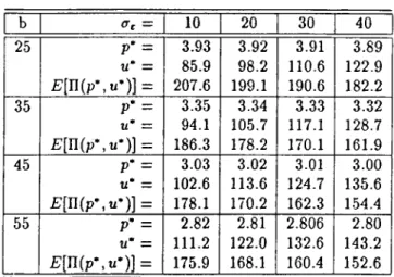
Lau L· Lau [22] studied the same problem using a normal forecast error distribution with zero mean and The only difference in their model is that they assumed a unit salvage value instead of a unit holding cost. Letting h = —0.5 and retaining the rest o f the parameter values in the above consideration, we obtain the results listed in Table-4.2. On the other hand, Table-4.3 shows their results for the same parameter set. Comparing Table-4.2 and Table-4.3 we see that two different forecast error distributions yield similar results. Also, the discussion above o f Table-4.1 is true for their case.
CHAPTER 4. EXAMPLES 21 b A = = 0 0 17.32 10 34.64 20 51.96 30 69.28 40 25 P* = li* = E [n(p*,u*)] = 3.940 73.500 216.090 3.913 81.887 197.291 3.886 90.190 178.528 3.859 98.406 159.802 3.830 106.531 141.113 35 P* = ti* = f:[n (p*,u *)] = 3.357 82.500 194.464 3.333 89.904 176.527 3.309 97.216 158.630 3.284 104.432 140.775 3.259 111.547 122.962 45 P" = li* = E[U(p\u^)] = 3.033 91.500 186.050 3.012 98.261 168.686 2.990 104.930 151.364 2.968 111.502 134.084 2.946 117.973 116.848 55 p* = u* = f ;[ n ( p * ,« ')] = 2.827 100.500 183.641 2.808 106.809 166.686 2.789 113.028 149.772 2.769 119.153 132.900 2.749 125.180 116.070
Table 4.1; Results o f Example-1.
c = \,b = 0 .5 , s = l , r = 0 , a = 102,
CHAPTER 4. EXAMPLES 22 b A = <Tt = 0 0 17.32 10 34.64 20 51.96 30 69.28 40 25 P* = u* = E[U(p\u^)\ = 3.940 73.500 216.090 3.936 87.025 208.406 3.931 100.543 200.722 3.927 114.054 193.040 3.922 127.557 185.359 35 p· = u* = E [n (p*,«*)] = 3.357 82.500 194.464 3.353 95.470 186.927 3.349 108.432 179.392 3.345 121.384 171.858 3.340 134.327 164.324 45 P* = u* = £ [ n ( p - ,« - ) ] = 3.033 91.500 186.050 3.029 104.087 178.616 3.026 116.663 171.184 3.022 129.229 163.752 3.018 141.786 156.323 55 P* = u* = E [n (p*,«*)] = 2.827 100.500 183.641 2.824 112.805 176.283 2.820 125.100 168.926 2.817 137.384 161.571 2.813 149.657 154.218
Table 4.2: Results o f Example-1.
c = l,/i = -0.5, s = l,r = 0,a = 102,
CHAPTER 4. EXAMPLES 23 b a, = 10 20 30 40 25 P' = 3.93 3.92 3.91 3.89 u* = 85.9 98.2 110.6 122.9 P [n (p * ,u ')] = 207.6 199.1 190.6 182.2 35 P* = 3.35 3.34 3.33 3.32 u* = 94.1 105.7 117.1 128.7 P [n (p -,u *)] = 186.3 178.2 170.1 161.9 45 P* = 3.03 3.02 3.01 3.00 u* = 102.6 113.6 124.7 135.6 E[U(p\u^)] = 178.1 170.2 162.3 154.4 55 P* = 2.82 2.81 2.806 2.80 u* = 111.2 122.0 132.6 143.2 f;[n (p * ,«* )] = 175.9 168.1 160.4 152.6
Table 4.3: Results o f Lau & Lau.
c = l , h = —
0.5,s = l , r = 0,a = 102,Pt = 1.6,Pu = 4,Pm = 2.8,
CHAPTER 4. EXAMPLES 24
4.2
Example 2
In this example, the previous assumptions are preserved. However, we assume that the forecast error has a price dependent uniform p.d.f.
S ( x ; p ) = \
m .(p -'a » 4 c ,
■ ‘
S « < 5 ("· (p -
+ a),
( 0, otherwise ,
(4.14)
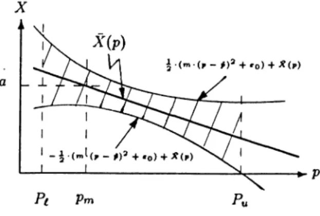
where rn,£:o ,and p > 0. Therefore, we require that the forecast error is minimized at p and it is increasing away from it. Note that, with this adjustment we bring a flexibility to the price dependency of the forecast error distribution. For example, by letting p = Pi we imply the condition that the range o f forecast error values increases quadratically in p. In this regard, possible realizations o f price-demand values are shown in Figure-4.2.
Figure 4.2: The Cross-Hatched Area Represents the Price-Demand Values That Can be Realized Under the Assumptions (4.2) and (4.14) .
Evaluating
G{x\p) = ^ +
2
m ( p - p ) 2 + e o
from (4.14) and taking r = 0 in (3.10) it follows that.(4.15)
Moreover, evaluating
CHAPTER 4. EXAMPLES 25
from (3.5) and (4.16), and using it in (3.4) we obtain
£ ’[n(p,u·)] = c - r + ( p - c ) - J V ( p )
- ^ • ( m ( p - p ) 2 + i:o ) (c + h)-(p + s - c)
(p + s + h) (4.18)
Differentiating (4.18) w.r.t. p once and twice we get
('P (p + s + h) 1 / / , (t + * ) ’ (4.19) d^E[n(p,u')] 5p2 = —2*6 — 77
i
(c -f h) m (c h)^ (p -f 5 -f h)^ -f h) {2 p + s + /i) -f p + (4.20)We can use (4.19) and (4.20) in a functional analysis to determine p* which maximizes (4.18). For details see Appendix-E.
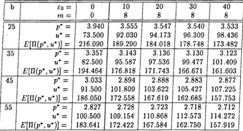
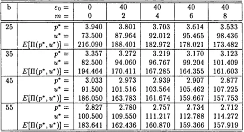
Table-4.4 and Table-4.5 display the numerical results obtained for the same parameter set used in Example-1 with the following additions
p = 1.5,
£o = 10,20,30,40, m = 2 ,4 ,6 ,8 .
Similar conclusions can be drawn ais in the first example. An additional observation is the considerable change in p* from its riskless value in Table-4.4. This agrees with the conclusion we made for Example-1.
CHAPTER 4. EXAMPLES 26 b 1 Co = m = 0 0 10 8 20 8 30 8 40 8 25 P‘ = U* = E[U(p',u-)] = 3.940 73.500 216.090 3.555 92.030 189.290 3..547 94.173 184.018 3..540 96.309 178.748 3.533 98.436 173.482 35 P' = u* = E [n (p -,u -)] = 3.357 82.500 194.464 3.143 95.587 176.818 3.136 97.536 171.743 3.130 99.477 166.671 3.123 101.409 161.603 45 P* = u* = £ ’[n(p-,u*)] = 3.033 91.500 186.050 2.894 101.809 172.558 2.888 103.622 167.619 2.883 105.427 162.685 2.877 107.225 157.753 55 P* = ti* = r [n (p * ,u ’ )] = 2.827 100.500 183.641 2.728 109.154 172.422 2.723 110.868 167.584 2.718 112.573 162.750 2.712 114.272 157.919
Table 4.4: Results o f ExampIe-2.
c = l,h = 0.5, s = l , r = 0,a = 102,
CHAPTER 4. EXAMPLES 27 b ^0 = 777 = 0 0 40 2 40 4 40 6 40 8 25 P’ = U* = E [n (p*,«*)] = 3.940 73.500 216.090 3.801 87.964 188.401 3.703 92.012 182.972 3.614 95.465 178.021 3.533 98.436 173.482 35 P* = U* = E [n (p * ,« ')] = 3.357 82.500 194.464 3.272 94.060 170.411 3.219 96.767 167.285 3.170 99.204 164.355 3.123 101.409 161.603 45 P' = u* = f:[n (p -,u -)] = 3.033 91.500 186.050 2.973 101.516 163.783 2.939 103.564 161.674 2.907 105.462 159.667 2.877 107.225 157.753 55 P* = U* = E [n(p*,u*)] = 2.827 100.500 183.641 2.780 109.550 162.436 2.757 111.217 160.870 2.734 112.788 159.366 2.712 114.272 157.919
Table 4.5: Results o f Example-2.
c = 1, /) = 0 .5 , s = 1, r = 0 , a = 102,
CHAPTER 4. EXAMPLES 28
4.3
Example 3
In this case we allow for an additional set-up cost (AC = 3) and an initial stock (r = 100) for the problem defined in Example-1.
Since M {u,p) = — u)] and the presence of initial stock does not alter the optimal decisions for the problem (3.30), we can use Table-4.1 to obtain (u,Pu) values directly. It
o
remains to compute Pr from (3.44) in order to run the procedure (3.45). The certainty values are computed by solving (3.22) where we place a set-up cost in the function (3.21).
The numerical results we get for our problem are displayed in Table-4.6. The class ★ indicate the optimal procurement values which turned out to be less than the initial stock. Therefore, w’e do not order but we set a price which maximizes the expected profit at a beginning stock o f 100. For the class o we have optimal procurement decisions being greater
o ^
than the initial stock. However, when we add AC = 3 to M (u,Pu) we obtain larger values
o o
than M{r,Pr). For that reason we do not order but we set the price to Pr. Finally, for the
o - . o
class · we order up to v and set the price to P^.
For
5
= 0,/i = 0 and no set-up cost case Mills [3] showed that the optimal price can not be higher than the certainty price, p*. This behaviour is also observed for our example problems where s and h are nonzero. See Table-4.1 through Table-4.5. However, we see in Table-4.6 that the presence of a fixed set-up cost violates this conclusion. Also, we have stated for Example-1 that the optimal price slightly declines as uncertainty in the problem is increased. But, it is seen in Table-4.6 that this is not true for the do not order case.Finally, in Example-1 we have concluded that uncertainty favours holding more stocks than the certainty stock u*. However, this conclusion is also violated by the presence o f a fixed set-up cost. See for instance, u* values for 6 = 55 in Table-4.6.
CHAPTER 4. EXAMPLES 29
Table 4.6: Results o f Example-3.
c = 1, K = S,h = 0.5,s = l , r = 100,a = 102,
Chapter 5
S U M M A R Y A N D
CONCLUSIONS
Upon setting our assumptions, we derived a mathematical expression for the expected profit in terms of the decision variables. In order to make it attractive for theoretical anal yses we studied this function in detail. Then, we formulated the optimization problem to determine the optimal decisions for maximizing the expected profit. By employing functional analyses we proposed a general solution procedure for the problem. We supplied numerical evidence for the applicability of this procedure by solving three different examples.
We also discussed the certainty profit. In Example-1, we proved that in general it con stitutes an upper bound for the uncertainty profit. For r = 0 and linear X {p) we obtained the optimal procurement and pricing decisions.
For an additional set-up cost, we showed that we can utilize an {s^S) type policy to obtain the optimal decisions. This policy is related to the clcissical (5,5) policy in a sense that we determine the optimal procurement by operating over the curve M (u,pu)· Moreover, we determine the optimal price as a by-product.
We believe that, with this theoretical study we explain major issues related to the one- period problem. This was our intention to start with so that, we would have a basis to extend the theory. An essential feature of the study is the proof o f optimality of an (5,5) type policy. This has useful implications for the multi-period case. Yet, another feature was the analytical approach to handling the price dependence.
Appendix A
First consider the following two integrals
/
Jci ■ti-X(p) (p) [u - X (p ) - y] · (y ; p) · rfy = [ u - A ^ ( p ) - y ] - G ( y ; p ) q ; )u-X'(p) ru-A'(p) + / G{y\P)dy (p)/
Jci y.u-AT(p) / G {y;p )d y, and, /•C3(p) _ /fa(p)/
[ y - w +A' ( p) ] y( y; p) dy =
/
[ y - « + A(p)]
J u - X ( p ) ■9(y;p)dy u - A ' ( p )pU-A.
f t i ( p ) _ i-u-Xi p) = / y-9
i y , p ) - d y - u + X(p) + / ^ (y ;? ) Ai(p) Ai(p) (A .l) [y - u + A (p)] y(y;p ) <fy¿y
¡■u-X(p) = - u + X { p ) + G{y\p) d y . (A.2)Therefore, substituting (A .l) and (A.2) in (3.4) we obtain
r [n (p ,
r u - X ( p )
u)] = - s A'(p) + ( p + s - c) u + c r - (p + s + /j)· / G {y;p) dy . J‘ i(p)
(A.3)
Appendix B
The 0 (w ,p ) function given by (3.6) is an important term wliich appears in all functional analyses. Therefore, its meaning and behaviour should be studied before going into detailed analyses. Two alternatively meaningful representations of 0 (u ,p ) are given below.
I G (y ,p )d y , (B .l)
* i(p)
= / F {x-,p)dx. (B.2)
Equation (B .l) involves the forecast error distribution, and equation (B.2) uses the demand distribution induced by (A8). Note that, in (B .l) the lower and upper limits o f the integral as well as the integrand may depend on price, whereas only the upper limit is a function of the procurement quantity u. A useful treatment is to see the integrals (B .l) and (B.2) over a plot. See Figure-B.l below.
It is clear with (B .l) and (B.2) that 0 (u ,p ) is positive for all feasible u and p, that is :
0 ( u , p ) > O , Vu,p. (B.3)
Furthermore, the first derivative o f 0 (ii,p ) with respect to p and u becomes
dQju^p) du ^Q(ti,p) dp = G{u - A '(p);p) = F (t/;p), dX{p) dp n-X{p) rU-A G ( t i - A '( p ) ; p ) + / dG{y;p) dp ■dy, = f d F {x;p) ( p ) + X ( p ) dx. (B.4) (B.5) (B.6)
For a general demand distribution, it is not possible to study the behaviour of the deriva tive o f 0 (ii,p ) w.r.t. p. It is evident in (B.6) that, besides the integrand, the limits of the
APPENDIX B. 33
G{y\p)
(a)
F (x ;p )
(b)
Figure B .l: (a) The shaded area is the expected value o f the forecast error which is known to be zero. The cross-hatched region is 0 (u ,p ) given by (B .l). (b) The shaded area is the expected value o f the demand which is known to be A'(p). The cross-hatched region is 0 (u ,p ) given by (B.2).
APPENDIX B. 34
© (u ,p )
^2(P)
Figure B.2: A General 0 (w ,p ) Function in u.
integration plays a role in this behaviour. This is the mojor drawback in making a theoretical generalization for the overall problem. Nevertheless, we still can make some assertions for the 0 (u ,p ) function :
Utilizing the information supplied by (B.4) we obtain
dQ{u,p) 0 < du dQ(it,p) du = 0 < 1 dQ{u,p) du for u < e i { p ) + X (p), for (p) + X (p) < u < d ip ) + X (p), for C
2
(p) + A'(p) < u.Using (B .l) and considering Figure-B.l.(a) we have
/•ia(p)
i(p)
f^Av)
/ C {y ;p )d y = C2(p) = © (e
2
(p) + A '(p),p).Again from (B .l) it follows that
0 (u ,p ) = O for w < -f-A (p ),
0 (ti,p ) = ti - X (p ) for ¿:
2
(p) 4 -X (p ) < u.Therefore, we can plot a general 0 (u ,p ) function w.r.t. u as in Figure-B.2. Considering the figure we have
APPENDIX B. 35
e(u,p) < u ,V u , p , (B .8 )
e(u,p) = o ,v p , and 0 < « < Ci(p) + A ( p ) , (B .9 )
0 ( u , p ) < u - e i ( p ) - A ' ( p ) ,Vp, and « > f i ( p ) + A ( p ) , (B.IO)
e(u,p) = u - X(p) ,Vp, and « > e2(p) + A ( p ) , ( B . l l )
e ( u , p ) < [u - £i(p) - X{p)]-t2(p) e2 {p )-€ \ {p )
{
Vp, and + A'(p) < u < e2(p) + A '(p ), 0 ( « , p ) > G (0;p) [u - A (p )] + / G{y\p) dy ,Vp,t/. ‘'ci(p) (B.12) (B.13)Consequently, we can say that 0 (u ,p ) is a convex function in u, but it has a general behaviour in p. Given a special problem we can utilize (B.2) and (B.6) to study the price dependence of 0 (u ,p ). The conditions (B.7) through (B.13) are essential in attempts for generalizing the results involving 0 (ti,p ).
Appendix C
Utilizing (A8) and substituting y = x — we can rewrite (3.26) as
rti-X(p) L {u ,p )= h W ~ X { p ) - y ] - g { y ,p ) dy A .(p) f^Ar) + ( P + s ) · / [ y - w + A '(p )] p(y;p)-dy J u - X ( p ) which becomes L {u ,p )= h G {y ;p )d y + {p + s ) [ X { p ) - u ] ‘'fi(p) fU-X{p) + ( P + s ) · / G {y ,p )d y Jtdv)
by using ( A. l ) and (A.2) in (C .l). Therefore, from (3.6) we obtain
L{u,p) = (p + s) [A'(p) - u] + (p + s + /i) 0 (u ,p ).
(C .l)
(C.2)
(C.3)
Appendix D
Using (4.2) in (4.9) we obtain
d^E[U(p,u’ )] _
dp^ _ 2 . 6 + 2 ± i £ ± ^^ ( p + S + / , )3 >
and it follows that
d^E[Y[{p,u‘ )] < 0 ■<=> p > p~ where P = y i c ^ h f 1/3 - (s + /»)· ( D. l )
Therefore, £ “[II(p,u*)] (which is given by (4.7)) is found to be convex for 0 < p < p” and concave for p > p“ .
From (4.8) we obtain p = p such that,
a g [n (p ,u ·)]
Qp
l p ^ - = a - t ( P - P m ) - 6 ( P - c ) - 4 ^ ^ ^ i ^ = 0 (D.2) (P + s + h yO
where p is the largest root of (D.2).
Consequently, we determine the minimizer p* of £ ’[11(p, u*)] from the following procedure:
APPENDIX D. 38
0
)
(ii) (Hi) (iv) if p“ < 0 then set p“ = 0. if p“ < Pt then : • if Pi <p< Pu then set p* =p,o else if E[U{Pi,u*)] > then set p* = Pi else set p* = P^.
if Pi < p~ < Pu tlien :
o o
• if p~ < p < Pu then set p\ =p,
o else if £ ’[n (p ", u*)] > £'[Il(Pti, w*)] then set p\ = p “ else set p\ = Pu·
• if E[U{Pi,u*)] > £'[n(pi,ii*)] then set p* = Pi else set p* = pi. if Pxi < p~~ then :
Appendix E
This material will closely follow Appendix-D.
From (4.20) we have
op^
where
<’ = l --- 2 6 + ™ (c + /0
J
'
Therefore, £^[II(p,ti·)] is found to be convex for 0 < p < p“ ,and concave for p > p . Taking
O
this into account and by equation (4.19) we obtain p from
5£7[n(p,u*)],
L /S.
\
/
( c + h ) - ( P + « - c)
— ~iE ----
A ( p ) - 6 ( p - c ) - m ( p - p ) - i --- ^
( P + « + /») - i ( m ( p - p ) 2 + £ - o ) - i i i ^ ) — = 0 (P + « + h)2 (E .l)where p is the largest root o f (E .l).
Consequently, p* can be obtained by the same procedure described in Appendix-D . Note that ¿ ’[[¡(p, ti*)] is given by (4.18) in this case.
Bibliography
[1] Von Neumann J., and Morgenstern O., ''Theory Of Games And Economic 5e-
/1
arioiir'’ ,Princeton University Press, (1944).[2] Oi W .Y ., "The Desirabiliiy Of Price InsiabilHy Under Perfect Competition^^ Economet- rica, Vol 29, 58-64, (1961).
[3] Mills E.S., "Price, Ontput, And Inventory Policy'\ John Wiley k. Sons,(1962).
[4] Hadley G. and Whitin T.M ., "Analysis Of Inventory Systems'", Prentice-IIall, Inc., Englewood Cliffs, N.J., (1963).
[5] Baron D.P., "Price Uncertainty, Utility, And Industry Equilibrium In Pure Competi tion", International Economic Review, Vol 11, No 3, 463-479, (1970).
[6] Baron D.P., "Demand Uncertainty In Imperfect Competition"", International Economic Review, Vol 12, No 2, 196-208, (1971).
[7] Sandmo A., "On The Theory Of The Competitive Firm Under Price Uncertainty" ,T\\o^
American Economic Review, Vol 61, No 1, (1971).
[8] Winkler R.L., Roodman G.M., and Britney R.R., "The Determination Of Partial .A/o- mcn/
5
” »Management Science, Vol 19, No 3, 290-96, (1972).[9] Leland H.E., "Theory Of The Firni Facing Uncertain Demand", The American Eco nomic Review, Vol 62, 278-291, (1972).
[10] Lev B., and Soyster A.L., "An Inventory Model With Finite Horizon And Price Changes', Journal of Operations Research Society, 30, 43-53, (1979).
[11] Atkinson A.A., "Incentives, Uncertainty, And Risk In The Newsboy Problem"", Decision Sciences, Vol 10, 341-357, (1979).
[12] Pasternack B.A., "Filling Out The Doughnuts ; The Single Period Inventory Model In Corporate Pricing Policif", Interfaces, Vol 10, No 5, (1980).
[13] Chandrasekhar D., "A Unified Approach To The Price-Break Economic Order Quantity (EOQ) Problem"", Decision Sciences, Vol 15, 350-358, (1984).
[14] Monahan J.P., "A Quantity Discount Pricing Model To Increase Venddor Profits"", Man agement Science, Vol 30, No 6, (1984).
BIBLIOGRAPHY 41
[15] Pasternack B.A., ^^Optimal Pricing And Rciurn Policies For Perishable Commodities^^
Marketing Science, 4(2), 166-175, (1985).
[16] Taylor S.G., and Bradley C.E., ''Optimal Ordering Strategies For Announced Price Increases'\ Operations Research, Vol 33, No 3, (1985).
[17] Lee H.L., and Rosenblatt M.J., "A Generalized Quantity Discount Pricing Model To Increase Supplier's Profits", Management Science, Vol 32, No 9, (1986).
[18] Banerjee A., "On A Quantity Discount Pricing Model To Increase Vendor Profits", Man agement Science, Vol 32, no 1 ,(1986).
[19] Dada M., and Srikanth K .N .,“ Pricing Policies For Quantity Discounts", Management Science, Vol 33, No 10, (1987).
[20] Gerchak
Y.,
and Parlar M., "A Single Period Inventory Problem^ With Partially Con trollable DemaniF, Computers and Operations Research, Vol 14, No 1, (1987).[21] Monahan J.P.,“ On Comments On A Quantity Discount Pricing Model To Increase Ven dor Profits", Management Science, Vol 34, No 11, (1988).
[22] Lau A.Hing-Ling, and Lau Hon-Shiang, "The Newsboy Problem With Price-Dependent Demand Distribution",HE Transactions, Vol 20, No 2, 168-75, (1988).
[23] Goyal S.K., and Bhatt S.K. "A Generalized Lot Size Ordering Policy For Price In creases", Opsearch, Vol 25, No 4, (1988).
[24] Kim K.H., and Hwang H., "An Incremental Discount Pricing Schedule With Multiple Customers And Single Price BreaP\ European Journal o f Operations Research, 35, 71-79, (1988).
[25] Abad P.L., "Joint Price and Lot-Size Determination When Supplier Offers Inci'emental Quantity Discounts", Journal O f Operational Research Society, Vol 39, No 6, (1988).