Electrical impedance tomography of translationally uniform cylindrical objects with general cross-sectional boundaries

(1)

IEEE TRANSACTlONS ON MEDICAL IMAGING, VOL. 9. NO. I . MARCH 1990 49

Electrical Impedance Tomography of Translationally

Uniform Cylindrical Objects with General Cross-

Sectional Boundaries

Y. ZIYA IDER, MEMBER, I E E E , NEVZAT G. GENCER, ERGIN ATALAR, HALUK TOSUN

Abstract-An algorithm is developed for electrical impedance tomography (EIT) of finite cylinders with general cross-sectional boundaries a n d translationally uniform conductivity distributions. The electrodes for d a t a collection a r e assumed to be placed around a cross- sectional plane; therefore the axial variation of the boundary conditions and also the potential field a r e expanded in Fourier series. For each Fourier component a two-dimensional (2-D) partial differential equation is derived. Thus the 3-D forward problem is solved a s a

succession of 2-D problems a n d it is shown that t h e Fourier series can be truncated to provide substantial saving in computation time. The finite element method is adopted a n d the accuracy of the boundary potential differences (gradients) thus calculated is assessed by comparison to results obtained using cylindrical harmonic expansions for circular cylinders. A 1016-element a n d 541-node mesh is found to be op- timal. F o r a given cross-sectional boundary, the ratios of the gradients calculated for both 2-D and 3-D homogeneous objects a r e formed. The

actual measurements from the 3-D object a r e multiplied by these ratios

and thereafter the tomographic image is obtained by the 2-D iterative equipotential lines method. The algorithm is applied to data collected from phantoms, a n d the e r r o r s incurred from the several assumptions of the method a r e investigated. The method is also applied to humans a n d satisfactory images a r e obtained. It is argued that the method finds a n “equivalent” translationally uniform object, the calculated gradients for which a r e the same a s the actual measurements collected. In the absence of any other information about the translational variation of conductance this method is especially suitable for body parts with some translational uniformity.

Keywords-Electrical impedance tomography; medical imaging; finite element method; cylindrical harmonics.

I. INTRODUCTION

LECTRICAL impedance tomography (EIT) is an im-

E

aging modality for which several clinical applications are being investigated [ l ] , [3]. However, the method can still only be used to obtain a difference image, i . e . , the difference in impedance distribution between two different conditions. For example, changes in impedance distribution in thoracic cross sections between end expiration and end inspiration are reconstructed. The purpose of this study is to extend the method to obtain “static,” i.e., actual images, as opposed to “difference” images.

Manuscript received January 30, 1988; revised July 10. 1989. This work was supported by the Middle East Technical University Research Fund (Projects AFP-86030 103, AFP-87030 103, AFP-88030 103 ).

Y . Z . Ider, N . G . Gencer. and H . Tosun are with the Department of

Electrical and Electronic Engineering, Middle East Technical University, Ankara, Turkey.

E. Atalar is with the Department of Electrical Engineering, Bilkent Uni- versity. Ankara, Turkey.

IEEE Log Number 8930705.

EIT, which is an inverse problem, aims at obtaining the internal impedance distribution of an object using data collected via electrodes applied on the surface. However, an essential part of all image reconstruction algorithms proposed for EIT at present [2]-[6], [14] is the solution of the forward problem, which is the calculation of the data, given the internal impedance distribution and also the boundary conditions imposed by the shape of the object and the electrodes.

Currents impressed by electrodes applied on the surface spread inside the object in three dimensions. Therefore the forward problem of EIT is a three-dimensional (3-D) problem and its solution requires a knowledge of 3-D boundary shape. The technique of obtaining “difference images,” as described in [2], is unique in the sense that it obviates the need for both cross-sectional and 3-D boundary information. However to obtain “static” images one must explicitly consider the 3-D shape of the object.

For the solution of the forward problem for an arbitrary boundary and general internal impedance distribution, a numerical technique is necessary. The finite element method (FEM) has been used by several investigators [SI, [6], [ l l ] . All of these studies have been confined to 2-D

applications and/or circular or rectangular boundaries [3], [ l 11. Furthermore, the requirements for an FEM algorithm for application to real situations in terms of mesh size, mesh generation for any boundary, and easy extension to three dimensions have not been investigated in re- lation to the imaging problem at hand.

In this study, an algorithm is developed for obtaining static tomographic images of cylindrical objects which have arbitrary cross-sectional boundaries. It is also assumed that conductivity is translationally uniform in the third (axial) direction. The relevance of these geometric assumptions to the actual use of the method is discussed. The method is assessed by obtaining images using data from 2-D and 3-D phantoms and also from humans.

11. DATA ACQUIS~TION HARDWARE A 16-electrode data acquisition system for EIT is developed. The system easily interfaces to a computer which has a 20-b parallel I/O port and which also has an AID converter. In this study an IBM PC/AT computer with an Intel 8255

U0

port and a 12-b, 25-ps A/D converter (Tec- 0278-0062/90/0300-0049$0 1 .OO @ 1990 IEEE

(2)

50 IEEE TRANSACTIONS ON MEDICAL IMAGING. VOL. 9. NO. I . MARCH 1990

mar) is used. It is possible to choose by software via the parallel port any two electrodes for application of 10 kHz and 1-5 mA current. Any other pair of electrodes can also be chosen to measure voltage differences. Any sequence of electrode selections with appropriate time delays can easily be programmed. To acquire the data presented in this paper, Brown et al. 's data collection protocol is used [2]. In this protocol, 16 electrodes are placed on the periphery of the plane of interest, and 16 pairs of adjacent electrodes are selected in turn to apply current. For each current pair selection, 13 voltage differences (gradients) are measured by selecting pairs of adjacent electrodes (ex- cluding the ones used for current application, because of the voltage drop on contact impedance) to be connected to a high-input-impedance differential amplifier. Because of reciprocity, only half of the total number of 208 measurements are independent.

It is known that tissue conductivity is constant up to 100 kHz; furthermore, in this frequency range displacement current is negligible in comparison with conduction current [13]. It is also known that at frequencies above 10 kHz neural stimulation thresholds are sufficiently high to allow for safe operation [13]. Therefore the 10-100 kHz frequency range is appropriate for EIT; and we have chosen the lower end of this range in order to ease the requirements on hardware design, especially those requirements relating to stray capacitive effects.

The 8255 control lines are isolated via opto-couplers. The 10-kHz current source and the 10-kHz voltage signal to be measured are transformer isolated from the applied parts. These precautions together with the use of an isolated power supply allow for application on humans. The isolated circuit common is connected to the object to decrease common mode signals. The signal detection block consists of a differential amplifier (CMRR

>

80 dB), a bandpass filter ( 1 0 +_ 2 kHz), a signal isolation transformer, a phase sensitive detector, and a computer-con- trolled amplifier (to adjust to a 50-dB dynamic range). Electrodes are selected by analog multiplexers, and electrode cable shields are signal driven to minimize inter- electrode capacitive coupling. For 2-D studies, a circular shallow container 1 cm in height is filled with NaCl solution, and a l-cm-thick agar block is placed at different locations. The conductivities of agar blocks were determined by a four-electrode technique applied to small rectangular samples taken from the blocks. For 3-D studies, cylinders which have arbitrary cross sections are used.

Electrode positions in the 2-D and 3-D phantoms are known exactly. Turbo-Pascal is used for the programming of data acquisition and for the algorithms for image reconstruction.

..Z

111. SOLUTION OF T H E FORWARD PROBLEM USING T H E

FINITE ELEMENT METHOD

A . Formulation of the 2 - 0 Problem

In EIT, the four-electrode method of impedance measurement is used because of the electrode contact impedance problem [2]. Thus, current is applied through two

electrodes of finite length placed on the boundary, and potential differences between other electrodes on the boundary are measured. For a 2-D problem, finding nu- merically the potential differences on the boundary for a given current electrode pair selection requires first the solution of the following equation:

VI * ( c V , U ) ( x , Y ) = 0 (x, y ) E S. ( 1 )

Here,

J on the surface of positive current electrode

c - =

an

au

r

0 elsewhere on the surface.

- J on the surface of negative electrode

S is the closed surface to be imaged; C is the boundary of S; U ( x , y ) is the potential distribution in S and on C;

a U / a n is the gradient of potential distribution normal to C; J is the current density on the electrode surface; and

c(x, y ) is the 2-D conductivity distribution in S .

In this equation, c V , U , i.e., conductivity times the electric field, represents the internal current density and merely expresses Ohm's law. For a conductive medium without any free charges, this current density must be so- lenoidal, i.e., its divergence must be zero; hence (1) is obtained. Thus, finding the distribution of the potential field within an inhomogeneous conducting medium through which steady current is flowing is equivalent to solving (1) subject to the Neumann boundary conditions as expressed above.

To obtain a FEM solution, the region to be imaged is divided in50 M triangular elements corresponding to N

nodes. If V is the N x 1 vector of unknown node potentials and c I , c 2 , *

. .

, c,,,, are the assumed uniform con-

ductivities of the M elements, it can be shown that [lo]

A ? =

b"

where

b'

is the

N

X 1 vector incorporating the boundary conditions, and A is a sparse

N

x

N matrix whose entries depend also on the element conductivities.

The solution for the potential distribution in S and on

C with respect to a refereyce node, provided that the corresponding row of A and b is modified to make A nonsin- gular, is

+

V = A - ' ; . ( 3 )

The vector of surface potential differences,

2,

which corresponds t? the actually measured variables can then be related to V through a matrix D by the equation

=

03.

(4)

The quantity

g'

is a 13 X 1 vector for each current electrode pair selection. Fig. l(b) displays the definitions for g1, g2, * *

.

, g I 3 for a certain electrode selection. Here-

after, the elements of

2

will be referred to as gradients. The matrix

D

is a very sparse matrix in that each row of

D has two nonzero elements. If the ith gradient is defined as the potential difference between the jth and kth node

(3)

IDER PI < I / . . ELECTRICAL IMPEDANCE TOMOGRAPHY Boundary Volt age Differences 91 SI

FEM FEM FEM

1

T a n s i o n ~ 1016 ~ 248 ~ 56

1

47.90 1 47.90 1 48.58 1 54.i1 Method elements elements elements

J mvolts) I (%) (%U) 1

+ 93 -

+

9,

96

g7

(b)

Fig. 1. Meshes used for the finite element method of solving Laplace's equation for a circular region. (a) An 56-element mesh, with element

numbering also shown. (b) A 1016-element mesh, for which element

numbering is principally the same as in the other mesh. This mesh has 541 nodes.

6.12

I

6.18 ~

potentials, then the ith row of D has

+

1 as itsjth element and - 1 as its kth element.

g12

913

B. Mesh Generation and Accuracy of the Forward

Solution

The accuracy of the solution for field distribution depends very much on the selection of a proper mesh. Fig. 1 shows a coarse and a fine mesh used to divide the region

S into finite elements. In fact, three meshes with 56, 248, and 1016 elements were used to solve the FEM equations. These meshes, with different numbers of concentric circular divisions, are easily generated by software [6].

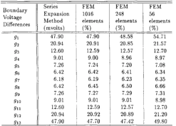
The gradients obtained for the three meshes for a certain current application to a uniform circular region (Fig. 1) are compared in Table I to the exact solution obtained by a series expansion method. The series expansion method is explained in Appendix A. It is observed that with the 1016-element mesh the gradients are correct to within 1 % . With the other coarser meshes the solution is not accurate near the site of current application. The 1016- element mesh, which has 541 nodes, is therefore adopted. The solutions given in Table I are obtained with the assumption that current is applied via infinitely thin electrodes located at the corresponding nodes. To understand the extent to which electrode width affects solution accuracy, the series expansion method is applied for different widths of the electrodes. It is found that if the elec-

' 20.94

,

47.90

TABLE I

BOUNDARY POTENTIAL DIFFERENCFS A S C A L C U L A T F D BY T H E FEM W I T H

DIFFERENT MESHES AND BY T H E SERIES EXPANSION M t r H O D

20.91 12.59 9.00 7.24 6.42 6.19 6.45 7.27 9.01 12.59 20.92 47.70

1

20.85 1

1

8.96 7.20 6.41 6.23 9.01

1

1 2 . 5 i , I 20.89

1

47.42 ~ 21.57 12.70 8.97 7.08 6.34 6.35 6.66 7.31 8.98 12.70 21.20 49.80 Boundary potential differences (gradients) obtained with series expansion method and FEM with different numbers of elements. The region has uniform conductivity of 0.20 S / m , and 1 mA of current is applied.

trode width is less than 1/64 of the circumference, gradients differ less than 1 % from the impulsive case. For different electrode widths, the field distribution in the vicinity of the current application electrodes must obviously be different. However, an advantage of the four-electrode impedance measurement method is that, since voltage difference measurements are made between other electrodes, the effect of current electrode width is not sensed, provided that electrode width is less than 1 /64 of the circumference.

Gradients measured from a 2-D phantom of circular geometry and uniform conductivity are compared with the calculated values using FEM. It is observed in Table I1 that the ratios of measured and calculated values are not significantly different for different measurement electrode pairs. The nonzero standard deviation of the measured gradients is due to the cumulative effects of errors caused by mesh size and electrode width, as well as errors com- ing from phantom construction and hardware inaccura- cies, noise, and digitization.

Fig. 2 shows the equipotential lines beginning from the voltage measurement electrodes calculated by using the FEM. These equipotentials are virtually identical to the ones calculated by the series expansion method. This is very important for the inverse solutions explained later.

Due to the large number of elements and nodes, the actual implementation of the FEM requires a large memory and significant amounts of computation time. The mesh generation algorithm and the methods used to solve the FEM equations are the critical components of any FEM solution.

The meshes shown in Fig. 1 are easily generated for a desired number of concentric divisions. Software is also developed to adapt a mesh generated for a circular region to any geometry. The method of mesh adaptation is given in detail in Appendix B. Fig. 6(a) shows a mesh constructed with this method for a noncircular cross section. The frontal algorithm is used to solve the FEM equations [7]. This algorithm is very memory efficient. The

(4)

IEEE TRANSACTIONS ON MEDICAL IMAGING. VOL. 9. NO. I . MARCH 1990 52

TABLE 11

MEASURFI) A N D CALCULA r E D B O U N D A R Y POTENTIAL DlFFtRENCES Boundary Voltage Differences 91 92 93 94 95 Q7 98 99 910 911 912 913 96 Measured (mvolts f s.d) 38.10 f 1.40 17.13 f 0.62 10.39 f 0.29 7.44 i 0.23 5.98 f 0.16 5.28 f 0.15 5.08 f 0.16 5.28 f 0.14 5.97 f 0.19 7.43 f 0.22 10.3s i 0.30 17.14 i 0.63 3S.06 1.32 Calculated (mvolts) 47.90 20.91 12.59 9.00 7.24 6.42 6.19 6.45 7.27 9.01 12.59 20.92 47.70 __-- Measured Calculated (mvolts f s.d) 0.80 f 0.029 0.82 f 0.029 0.83 f 0.023 0.83 5 0.026 0.83 f 0.022 0.82 f 0.023 0.82 f 0.026 0.82 f 0.022 0.82 f 0.026 0.82 f 0.024 0.82 k 0.024 0.82 f 0.030 0.80 f 0.027 Measured and calculated boundary potential differences are compared for a circular region of uniform conductivity. Calculated values are for I mA current to a circular region of 0.20 S/m conductivity. Since measured values were not from an exactly 0 . 2 0 S/m region, ratios were taken for comparison. Standard deviations of measurements are obtained by considering all 16 current applications.

Fig. 2. Equipotential lines obtained by FEM (1016 elements) for a uni- formly conductive circular region. Current is applied between the two electrodes shown.

memory requirement of the frontal algorithm depends very much on the numbering of the mesh elements. By using a numbering strategy of the type shown in Fig. l(a), the RAM memory requirement is reduced to only 4 kilobytes. For each current application the FEM equations must be solved. These 16 sets of equations are simultaneously solved using the frontal algorithm in 9 min using an 4.77- MHz IBM-AT with the 80287 coprocessor. A period of 3

min is required for initial file preparations and therefore a second set of equations can be solved in only 6 min. C. Formulation of the 3 - 0 Problem f o r a Finite Cylinder of Arbitrary Cross Section with Translationally Uniform Conductivity

For a finite cylinder of height 2a and diameter d (Fig.

3), the problem can be reduced to the solution of a series of 2-D problems by making use of Fourier expansions. Since the current electrodes are placed at the

z

= 0 plane, and since a symmetric cylinder is used, this boundary condition can be expanded in cosine series (without loss

Fig. 3 . Finite cylinder along z axis. The distance from the origin to the

top is represented by U .

of generality); hence the solution can also be expressed as

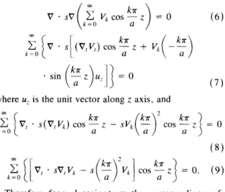
With V and V, being the 3-D and 2-D Laplace operators and s being the 3-D conductivity distribution,

kx U

1

( k = O 03

v

*

sv

c

vkC0s-z

= o

ka k = O

5 [v

.

+V,V,) cos - a

z

+ v,

( 7 ) where uz is the unit vector along

z

axis, and

k = O U

k = O

Therefore, for each cosine term, the corresponding coefficient must be zero:

v,

* SV,Vk - s

(:T

-

v,

= 0.

Each component Vk obeys a different 2-D partial differential equation with parameter ( k a / a ) 2 . The boundary condition for each equation can also be found:

must be obeyed, and

m SA(: an k = o =

c

JkC0s-z kn ( 1 2 ) a k = O a or

where

Jk

is the coefficient of the kth term in the cosine expansion of the boundary condition.

(5)

53 0.992 0.427 0.249 0.166 0.132 0.126 0.132 0.166 IDER er a l . : ELECTRICAL I M P E D A N C E TOMOGRAPHY

1 . 4 1 0.983 0.431 0.245 0.167 0.133 0.124 0.133 0.167 0.554( \ \ \ k 2

A:::

1.15 1.00 0.85 0.70

Fig. 4. Gradient values obtained by solution of equation (10) for eight frequency terms for a cylinder of circular cross section, with diameter 20 cm and height 80 cm. For the 0 frequency term all gradient values are multiplied by 1.3/0.59. k represents the frequency index in (10). Units

are arbitrary.

In order to determine the number of terms to be used, gradients obtained for different terms are calculated and are shown in Fig.

4.

It is found that at higher frequencies, i.e., higher k values, gradients are much lower. Further-

more, for higher k values, the rate of decrease of gradients further from the current electrodes increases. Therefore, convergence of the sum can be tested by looking at the maximum contribution of each new frequency term. In this study, solution is stopped after the frequency whose maximum contribution to the sum is less than 1 % . It is found that eight frequency terms are sufficient for convergence.

Therefore by adopting this approach, it is possible to solve the 3-D problem by solving eight 2-D problems. This is an advantage of the four-electrode impedance measurement method where the high-frequency potential field, which is significant only near the current electrodes, is not of interest. The solution of eight 2-D problems takes a total computation time of 3

+

8 X 6 = 51 min. Of this,

3 min are for preparation of files that use mesh information for the solution of all the 2-D problems.

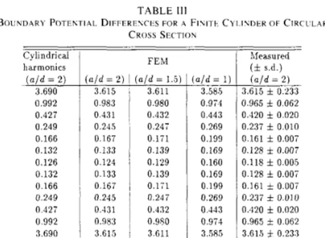
The accuracy of the solutions is tested against the cylindrical harmonic solutions for a circular cylinder. The cylindrical harmonic expansion method is explained in Appendix A. Cylindrical harmonic solutions for an a / d ratio of 2 are given in the first column of Table 111. FEM solutions are given in the other three columns for different a / d ratios ( 2 , 1.5, and 1, respectively).

The maximum percentage difference of the solutions obtained with the two methods, cylindrical harmonics and FEM, is less than 2 %

.

Comparison of FEM solutions for different a / d ratios shows that for a values more than twice the diameter of the cylinder, the gradient values do not significantly

TABLE I l l

B O U N D A R Y P O T E K T I A L D l F F E R E V C t S FOR A Fl'illt; CYl.lVDER OF C I R C L ' L A R C R O S S SECTION Measured ~ (f s.d.) FEbl Cylindrical

1

harmonics (a/d = 1.5) 3.611 0.980 0.432 0.24; 0.171 0.139 0.129 0.139 0 . l i l 0.24i 0.432 0.980 3.611 ( a / d = 1) 3.585 0.9i4 0.443 0.269 0.199 0.169 0.160 0.169 0.199 0.269 0.443 0.971 3.585 (uld = 2 ) 3.615 i 0.233 0.965 f 0.062 0.420 f 0.020 0.237 f 0.010 0.161 f 0.00; 0.128 i 0.007 0.118 f 0.005 0.128 f 0.007 0.161

*

0 . O O i 0.237 i 0.010 0.420 f 0.020 0.965 i 0.062 3.615 i 0.233 The first two columns show the cylindrical harmonics and FEM solu-

tions with the same u / d ratio. where 2a is the height and d is the diameter of the circular cylinder. The next two columns show the FEM solutions for different u / d ratios. Conductivity is taken to be uniform as 0.20 S / m . Units are mV. The last column includes the measurements from a circular cylindrical phantom filled with salty water so that the cr/d ratio is 2 . Stan- dard deviations of measurements are obtained by considering all 16 current applications. The measured values are scaled to match the highest gradient with the FEM solution for u / d = 2 .

change. Therefore, those gradient values obtained with an a / d ratio of 2 can be considered the solutions for an in- finitely long cylinder.

On the other hand, solutions obtained with a / d ratios less than I .5 (i.e., 1 ) differ very much from the solutions of an infinitely long cylinder, especially at the gradient values calculated at electrodes placed opposite to the current application electrodes.

IV. IMAGE RECONSTRUCTION-SOLUTION OF THE

INVERSE PROBLEM

In this study, the iterative equipotential lines method (IELM) [2], [4] is used to reconstruct images. In this method, first, the forward problem is solved for a homogeneous medium to calculate the voltage distribution so that the gradients and the equipotential paths which end on the voltage-measuring electrodes are determined. Sec- ond, the conductivity values between two consecutive equipotential lines are multiplied by the measured to calculated gradient ratio for the corresponding electrodes. The final conductivity distribution is calculated as the average of all such corrected distributions which are obtained for each current application. But since the calculated gradients for this final conductivity distribution do not satisfy the measured ones, this procedure is applied iteratively until the error between the measured and the calculated gradients reaches a reasonably small value.

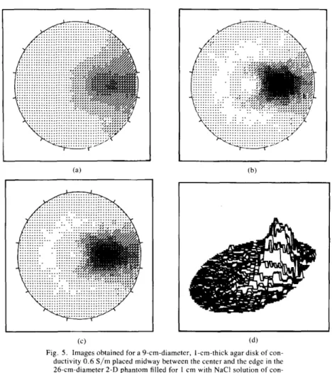
Fig. 5 displays the images obtained for a circular agar block of conductivity 0 . 6 S/m and diameter 9 cm, placed midway between the center and the periphery of the 26- cm-diameter 2-D phantom filled with liquid of conductivity 0.21 S/m. Both the 2-D phantom and the electrodes used have 1 cm thicknep. It is observed that even the first iteration yields an image which is indicative of the position and relative size of the object. However, both con-

(6)

54 IEEE TRANSACTIONS ON MEDICAL IMAGING. VOL. 9, NO. I . MARCH 1990

Fig. 5 . Images obtained for a 9-cm-diameter, l-cm-thick agar disk of conductivity 0.6 S/m placed midway between the center and the edge in the 26-cm-diameter 2-D phantom filled for 1 cm with NaCl solution of conductivity 0.21 S/m. (a) Result of first iteration. (b) Results of fifth iteration. (c) Result of tenth iteration. (d) Result of tenth iteration drawn in the perspective mode. Parts (A), (B), and (C) are drawn in the inten- sity mode with ten intensity levels covering the range o f 0 . 18 to 0 . 5 S/m.

trast and resolution increase considerably with further iterations. The rms value of the percent differences between measured and calculated gradients is calculated at the end of each iteration to monitor the convergence of the algorithm. This rms value has a minimum at about 3 . 5 % around the tenth iteration. However, further iterations cause an increase in this rms value, indicating divergent behavior. Therefore the IELM does not give a conductivity distribution for which the calculated gradients are exactly the same as the measured gradients. This property of IELM, which is true for even simulated data, has also been observed by Yorkey

[4].

Average conductivity values for the flat tops of the regions in Fig. 5 corresponding to the agar object at the first, fifth, and tenth iterations are 0.35, 0.49 and 0.58 S/m. These results show that, for quantitative imaging, iterative application of the method is very important. Conductivity of the background stabilizes at about 0.20 S

in a few iterations.

Reconstructing tomographic images of 3-D bodies is a somewhat different problem. It is in fact a problem of finding the 3-D conductivity distribution from the gra-

dients measured by electrodes placed around a certain slice of the body. This is so because off-slice objects also affect the data collected by such electrodes [12]. Yet, it is not possible to estimate the positions and conductivities of off-slice objects from the measurements collected around a slice. However if translational uniformity is assumed, then one may find a 2-D conductivity distribution whose translationally extended form yields a gradient set which satisfies the original measurements. However, one can find such a 2-D conductivity distribution if a 2-D equivalent form of the measurements is known. A 2-D equiv-

alent form of the measurements may be defined to be the data set one would measure for a 2-D object having a conductivity distribution the same as the transverse conductivity distribution of the translationally uniform 3-D object.

The 2-D equivalent form of the measurements can be calculated by multiplying the measurements by the 2-D/3-D ratio of calculated gradients obtained for the actual conductivity distribution. However, in this study, since the actual conductivity distribution is not known, the 2-D/3-D gradient ratios are calculated for a homogeneous

(7)

I D E R ef a l . : E L E C T R I C A L I M P E D A N C E T O M O G R A P H Y 55

conductivity distribution. Therefore, once the 2-Dl3-D gradient ratio is calculated, one can find an approximate 2-D equivalent form of the measurements and then begin to search for the 2-D conductivity distribution using IELM.

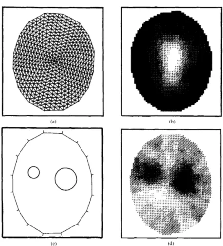
This approach gave satisfactory results for phantoms with translationally uniform conductivity distributions. A cylindrical phantom which does not have a circular cross section is constructed and is filled with salty water, and delrin rods are placed inside. Fig. 6(a) shows the mesh used for the solution of the field distribution and for image reconstruction. Fig. 6(b) shows the actual locations and sizes of the delrin rods. Fig. 6(c) is the reconstructed image of the delrin rods using the original data without multiplying by 2-D/3-D gradient ratios. In this image the positions of delrin rods cannot be seen at all. Finally, Fig. 6(d) is the reconstructed image using the 2-D equivalent form of the data. This image gives sufficient information about the sizes and the locations of the delrin rods. The percentage conductivity difference of delrin rods from the background is about 42 % .

The 2-D/3-D gradient ratios are also calculated for the reconstructed conductivity distribution, as shown in Fig. 6(d). It is found that these ratios do not differ more than 1 % from the ratios calculated for a homogeneous distribution. Therefore, the error incurred from using 2-D/3-D ratios for a homogeneous distribution is negligible. For very high contrast images, the error may not be neglected. However, even though an actual object may have regions with very different conductivity values, such as delrin and water in this case, the reconstructed images, because of the limitations of the IELM in particular and impedance tomography technique in general, have much lower contrast.

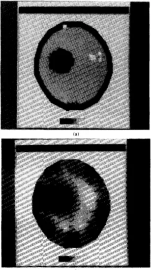
Tomographic images of the human arm are also reconstructed using this imaging system. The problem of finding electrode positions is first overcome by forcing the arm boundary to be circular, resulting in the use of pre- determined electrode positions. For this purpose, a ring is prepared which is 7 cm high and which has a diameter slightly less than the average diameter of the slice of interest of the arm. Electrodes are located inside the holes which are bored with equal distances on the inner surface of the ring. The arm is then inserted inside the ring until the electrodes reach the level of the slice of interest. Fig. 7(a) shows the fifth iteration of the tomographic image of a human arm, where the slice is chosen to be below the armpit of one third the distance from the armpit to the elbow. In the image, the large dark area and the brightest region probably correspond to the humerus and the blood vessels, which are known to run together in a collection at this level of the upper arm, respectively [9]. Another application is performed with the data collected from human arm using a noncircular ring which has a shape closer to the actual boundary shape of the slice of interest (Fig. 7(b)). The selected slice is again roughly the same as the one which was chosen for the previous case. Again the vessel group is identified; however the bone appears as more shifted to the boundary. In fact the bone was ac-

tually closer to the boundary when the noncircular ring was used, as tactually sensed by us. When these experi- ments were repeated to obtain images from multiple sub- jects, the following general features for the arm images were observed: 1) The Humerus appears rather close to the periphery and its contrast with respect to its surround- ing is low. In particular, the region between the bone and the periphery has low conductivity. 2) Low-conductivity regions extending inward from the boundary may be observed. 3) A high-conductivity small locality may be

identified as the vessel groap. 4) There is a tendency toward lower conductivity at the periphery with respect to the inner regions.

To properly interpret these images, cross-sectional anatomy atlases may be consulted. However, since EIT is limited in resolution one does not expect to obtain images which correspond to the anatomy in a millimetric scale. It is known that the equipotential lines method is a nonlinear reconstruction method and has a position-de- pendent point spread function [2J. Resolution of a prac- tical 16-electrode system is roughly found to be 7-10% of diameter [ 11, [2]. Furthermore, several reconstruction artifacts may be complicating the interpretation of EIT images. Therefore, a simulation study is undertaken to understand to what extent EIT can give reasonable images of the actual arm. Fig. 8(a) shows a simulation picture of the upper arm which is constructed in reference to standard anatomy books [9], [15]. The outermost low-con-

ductivity layer corresponds to the skin and the fatty subcutaneous layer, which can be a few millimeters to a centimeter thick. The bone, humerus, is slightly off-cen- tered, and bone marrow is also represented. Major vessels of the upper arm, the brachial artery, brachial vein, and basilic vein, run close to each other and are rather inter- nally located. On the periphery there is the large cephalic vein, and also we have assumed a more pronounced peripheral site with low conductivity in order to represent more localized fat depositions under the skin. The conductivity values for different tissues are taken as reviewed elsewhere [14]. The background tissue, which is mostly skeletal muscle, is assigned the average transverse conductivity of the human arm [ 141. The forward problem is solved for this 2-D simulation picture and the calculated gradients are accepted as data from which the EIT image shown in Fig. 8(b) is obtained, using the equipotential lines method.

It is observed that the low-conductivity outermost layer is not identified as a thin, well-defined layer but its effect is to generally decrease the conductivity of the relatively peripheral regions. It is observed that the low-conductivity bone region is therefore not found to have high contrast difference with respect to this peripheral region and it appears to be rather connected and shifted to the periphery. The blood vessel group is well localized, with a wide skirt, and of course individual vessels are not rec- ognized. The vessel group appears to be somewhat shifted away from the boundary. The peripheral vessel is not felt at all, and the peripherally localized fat is seen to generate a stripe artifact which extends into the region with de-

(8)

56 IEEE TRANSACTIONS ON MEDICAL IMAGING, VOL. 9. NO. I , MARCH l 9 Y O

Fig. 6 . (a) Mesh used for the finite element method in the solution of Laplace’s equation for the noncircular cross-sectional

geometry at hand. (b) Actual locations and sizes of the delrin rods placed in a noncircular finite cylinder. (c) Image recon- structed without considering the 3-D nature of the object. (d) Image reconstructed using the same data as in (c) but taking

into account also the 3-D effects. The fifth iteration image is shown.

Fig. 7. (a) Reconstructed image of human arm. Selected slice is below the armpit by one third the distance between the armpit and elbow of the right arm. Boundary of the cross section is forced to be circular by inserting the arm into a circular ring with inside attached electrodes. Nine gray levels from black to white are used to represent nine conductivity levels. (b) The same arm inserted into a noncircular ring which has approximately the same shape as the arm itself. Maximum difference in pixel values divided by maximum pixel value is 65 %.

(9)

IDER PI U / . : ELECTRICAL I M P E D A N C E TOMOGRAPHY 57

(b)

Fig. 8 . (a) Two-dimensional simulation picture of the upper right arm cross section below the armpit by one third the distance between the armpit and elbow ( u p p e r : anterior, lower: posterior. /eft: lateral, righr: medial). The same boundary as in Fig. 7 is assumed. The conductivity values of different tissues are taken as follows: 0.033 S/m for subcutaneous tissue. 0.025 S/m for fat tissue, 0.0066 S/m for bone, 0.04 S/m for bone mar-

row, 0.66 S/m for blood, 0.2 S/m for muscle. (b) Image obtained by

using the calculated gradients for the simulation picture shown in ( a ) . Maximum difference in pixel values divided by maximum pixel value is 85 %. Fifth iteration of IELM is shown.

creasing contrast and width. Therefore, even with noise- free 2-D simulation data, the anatomical boundaries may not be obtained in a clear-cut fashion. The striking simi- larity between the images obtained with simulation data and the actual data shows that the undesirable features observed in the actual images derive from the fundamental limitations of the equipotential lines method.

Finally, Fig. 9 shows an EIT image of the thorax at the mamillary level. The data are collected by the APT hardware, developed by Brown er al. [14] of Sheffield Uni- versity, U.K., which work at 50 kHz. This system is fast and therefore it is possible to collect the data in under 1

s

while breath is held at inspiration. A mechanical system is developed to determine electrode positions. Electrodes

Fig. 9. EIT image of the thorax at the mamillary level. Maximum difference in pixel values divided by maximum pixel value is 7 5 % . Upper boundary in the picture is the anterior surface. and the right side in the picture I S the left side of the thorax. Fifth iteration o f IELM is shown.

are held at the end of bars which may be slid until the electrodes touch the body surface. Angular and linear displacement of the bars may be marked so that electrode locations are later determined. In this thorax image the two lungs appear as low-conductivity regions. The heart and/or any other structure is not recognizable. The low- conductivity extension to the anterior surface is probably the stripe artifact of the sternum. This image also illus- trates the fact that the fundamental limitations of the IELM must be reconsidered for obtaining images of a complicated section such as the thoracic section shown here.

V . CONCLUSIONS A N D DISCUSSION A . The Finite Element Method Used

When static images are aimed at, as in this study, the forward solutions must be very accurate. In obtaining difference images using the equipotential lines method, con- sistent errors in the reference and actual data sets cancel when gradient ratios are taken. The requirement of accuracy for obtaining static images has caused us to use a mesh with a large number of elements. Furthermore we have used a mesh which is the same for all current applications and which has elements of almost equal size throughout the region. The reasons are:

Although a different mesh for every current application can be chosen such that small elements are used only near the current applying electrodes, some computational efficiency is lost. If only one fine mesh is chosen for all currents, then matrix A in (2) is the same for all current applications and only the right-hand side differs. Therefore the forward elim- ination phase of the solution algorithm need not be repeated for all currents [7].

In the FEM used in this study. every element must have uniform conductivity. The conductivity of an

(10)

IEEE TRANSACTIONS ON MEDICAL IMAGING. VOL 9. NO I. MARCH 1990

58

3)

. .,

element must then be assigned by averaging the corresponding image region. With small elements the averaging effect is not significant. Furthermore in the constant mesh since the elements are directly assigned conductivities, such an averaging is not required at all.

Resolution of a 16-electrode EIT is argued to be 7- 10% of the diameter [ l ] . The finite elements must be smaller than the smallest object detectable so that precise definition of object position is obtained. In this study the element dimension is about 3.3% of diameter.

All these considerations led us to the selection of the 1016-element mesh used in this study. The 248-element mesh gave unacceptable results, especially when the 3-D solutions were compared.

B. Solution of Forward Problem to Include 3-0 Effects The Fourier decomposition technique has several ad- vantages. First of all the problems of 3-D mesh generation and 3-D FEM formulation need not be tackled because the 3-D problem is solved as a succession of 2-D solutions. Second, a considerable saving in computation time is achieved. For a cylinder of height three times the diameter, if a 3-D mesh were generated with simple repe- tition of the 2-D mesh, then 90 different levels would have to be considered because the length of the elements in the third dimension must be comparable to their size in the transverse plane [ 101. This means at least a 90-fold increase in solution time, provided that the block diagonal nature of the FEM equations are considered. A more efficient mesh may of course be constructed, but in such an effort all of the constraints we have considered for 2-D mesh generation must be reconsidered. In the Fourier decomposition technique used here the time required for the solution for the 3-D forward problem is only eight times more than that for the 2-D problem. One important reason for achieving this computational efficiency is that the field solutions in the immediate vicinity of the current electrodes need not be known as

a

consequence of employing the four-electrode impedance measurement philosophy.

C. Assumptions Regarding 3 - 0 Properties

It may be argued that actual objects such as the limbs do not have exact cylindrical shapes. However, we have obtained images of the upper arm demonstrating that the cylindrical assumption is a good rule-of-thumb assumption. Thus the computational efficiency obtained by this assumption, especially in the absence of information regarding the 3-D geometry of the object, is worth consid- eration.

Another, more fundamental assumption of the method presented here is that of translational uniformity of conductivity. Actual objects may not satisfy this condition. However, it may be proposed that the images obtained in this study are “equivalent” images in the sense that, had the object had that particular translationally uniform conductivity distribution, then the gradient data to be obtained from it would have been the same as the actual data obtained. The contributions of off-slice objects to EIT im-

ages have been studied [12]. There seems to be no way to estimate the off-slice positions of objects from their contributions to an EIT image reconstructed from data obtained from equiplanar electrodes. Therefore we believe that in the absence of any other information regarding 3-D conductivity distribution, the method used here yields a reasonably equivalent image. This is so especially for the limbs where bones and vessels extend perpendicular to the imaging plane for considerable distances.

Before the above assumptions for 3-D shape and conductivity distribution are further evaluated, it will be necessary to study the capabilities of the IELM in reconstructing complicated body sections. Our simulation studies have shown that, in terms of resolution, the IELM is itself a major limiting component.

D. Electrode Positions

Finally, one must comment on the accuracy with which electrode positions must be known. If an

CY%

error in the angular separation between two adjacent electrodes is made, then the gradient calculated between these two electrodes is roughly in

CY%

error also. Such errors cause the appearance of higher and lower conductivity regions separated by the equipotential line for that particular electrode. The contrast error is found to be also about

CY%

near the boundary and less marked as the regions of conductivity artifact move toward the inside. Therefore in order to avoid such noticeable stripes near the boundary, electrode positions must be accurately known. A hard-

ware and/or software technique to find electrode locations easily when data are collected from an actual object is needed.

APPENDIX A

SOLUTIONS USING CYLINDRICAL HARMONICS

Solution of the Laplace equation for a finite cylinder of radius R which has translationally uniform conductivity c can be expressed using the cylindrical harmonics as

+ ( r , 0, z ) =

C

A,, sin (mO)rlll

+ C

C

A,,,,

m m m

in = I n = I m = I

with the boundary condition

where

4,

and electrodes.

are the angular locations of two current The unknown coefficients A,,n and A,,, are evaluated as

21, sin

(rn4,)

A,,,, = c1rm2aR”‘ ’ 21, sin ( m 4 , ) c I r a ( n a R / a ) Z,’rl(n7rR/a)’ Ann, n , m = 1 , 2 , - - e , 00. ( A . 4 )

(11)

IDER (’f a / ELECTRICAL I M P E D A N C E T O M O G R A P H Y 59

In

finding from its infinite series expansion, it is nec- essary

to

generate the modified

Bessel

function

I,,,

and its

tions are evaluated using their series expansions [8]. However, because of the large truncation numbers in- volved, Bessel functions of very high order need to be evaluated. Since I,,, and I:, asymptotically approach the

exponential function, for very large m the values of Z,fl and I;, may be prohibitively large for storage in the computer. For this reason, the asymptotic form of the ratio Zm/Ih for a fixed argument and for large m is needed. Using the asymptotic forms given in [8] for Zn1, the ratio Zm/Zh can be shown to be z / m , where I is the argument. Without dealing with infinitely large numbers for

Z

,

and

Zk

sepa- rately, we can work with the asymptotic ratio which is well behaved. Therefore, the ratio Zm/Ik was calculated for increasing m , using the series expansions for I,,, and

Z

;

until the ratio became close to the asymptotic value by less than 0.1 %. After this m , only the asymptotic value was used. For each n , the value m was incremented up to 10 000; n was incremented until each new term ceased to change the gradients by more than 1 %

.

Solution of the Laplace equation for a 2-D homogeneous circular region, with nonzero current electrode widths, can be shown to be

. I ..:.,- T,!~, .-:*I. -c - = c c t +- tLr nryllment The40 func-

[COS -

e))

- COS ( n ( a 2 -

e ) ) ] .

(‘4.5

1

For the above expression, a 1 and cy2 represent the an-

gular positions of current electrodes and

p

is the angular width of each electrode. The summation is stopped for

(

l/n2)(r/R)”

<

For r =

R,

( l / n 2 )

<

n

>

io3.

APPENDIX B MESH ADAPTATION

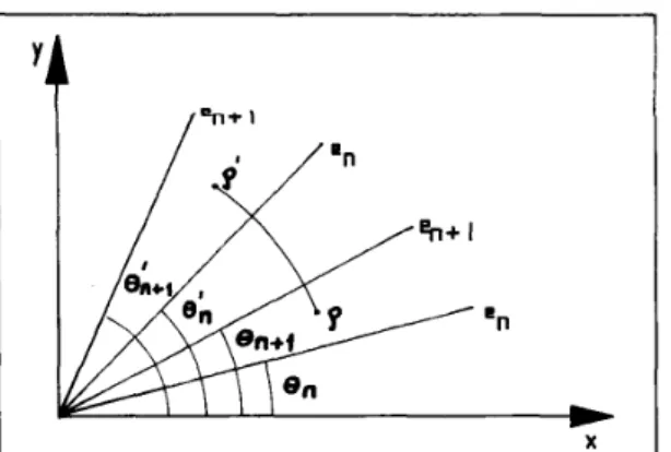
The electrode positions are expressed in polar coordi- nates with respect to a central reference point and the first electrode. The angles of the electrodes for a circular object and their distance from the central point are multiplied by appropriate factors to make them coincide with the electrodes of the actual object. The nodes of the circular mesh are also transformed using an interpolation formula (see Fig. 10):

Here, e,,: e, + I:

(r,,,

e,,)

is the nth electrode of circular mesh;

(r,, + I , 8, + I ) is the ( n

+

1 )st electrode of circular mesh which is adjacent to e,,;

‘f

/ % * I

I X

Fig. IO. Transforming the nodes of a circular mesh to obtain a mesh for noncircular cross sections.

p : e:,:

( r ,

e )

is a node of circular mesh such that

e,,

<

(r,,,

e,,)

is the nth electrode of the actual object;

(r:,+,, is the ( n

+

1)st electrode of the

( r ’ ,

e ’ )

is a node of the actual mesh such that 6

< e,+,;

actual object which is adjacent to e;; p ’ :

e:,

I

e,

I

e:,+I.

ACKNOWLEDGMENT the development of the EIT hardware.

The authors wish to thank C . Altan, who contributed to

REFERENCES

[ l ] B. H. Brown, D. C . Barber, and A . D. Seager. “Applied potential tomography: Possible clinical applications,” Clin. Phys. Physiol. Meas., vol. 6 , no. 2, pp. 109-121, 1985.

[2] D. C . Barber and B. H. Brown, “Recent developments in applied potential tomography-APT,” in Proc. 9th Con$ Inform. Process. in Med. Imaging (Washington, DC), 10-14 June 1985, pp. 106-121.

[3] A. D. Seagar, D. C. Barber, and B. H. Brown, “Electrical impedance

imaging,” Proc. Inst. Elec. Eng., vol. 134. pt. A, no. 2 , pp. 201- 210, Feb. 1987.

[4] T. J. Yorkey, J. G. Webster, and W . J . Tompkins, “Comparing re- construction methods for electrical impedance tomography, ” IEEE

Trans. Biomed. Eng., vol. BME-34, pp. 843-852, Nov. 1987. [5] Y. Kim, J. G. Webster. and W. J . Tompkins, “Electrical impedance

imaging of the thorax,” J . Microwave Power, vol. 18, pp. 245-257. 1983.

[6] T. Murai and Y. Kagayawa, “Electrical impedance computed tomography based on finite element model,’’ IEEE Trans. Biomed. E n g . ,

[7] B. M . Iron, “Frontal solution program for finite element analysis.” [8] M . Abramowitz and I . A. Stegun, Handbook of Mathematical Func- [9] P. Thorek, Anatomy in Surgery. Toronto: J . P. Lippincott Company

[ l o ] P. P. Silvester and R. L. Ferrari, Finite Elements for Electrical En-

gineers. New York: Cambridge University Press. 1983.

[ l I] A. Wexler, B. Fry, and M . R. Neumann, “Impedance computed to- mography algorithm and system,” Appl. Opt.. vol. 24, pp. 3985-

3992, Dec. 1985.

1121 J . Jossinet and G. Kardous, “Physical study of the sensitivity distribution in multi-electrode systems.” Clin. Phys. Physiol. M e u s . . vol.

[13] B. H. Brown, “Tissue impedance methods,” in Imaging with Non-

ionizing Radiations, D. F. Jackson, Ed. Surrey, UK: Surrey Univer-

sity Press, 1983, pp. 85-1 IO.

[14] D. C. Barber and B. H . Brown, “Applied potential tomography,” J . Phys. E: Sei. Instrum., vol. 17, pp. 723-733, 1984.

[I51 R. Warwick and P. L. Williams, Eds., Gray’s Anatomy. Edinburgh,

Scotland: Longman, 1973, pp. 540-542. vol. BME-32, pp. 177-184, 1985.

Int. J . Numer. Meth. Eng., vol. 2 , pp. 5-32, 1970.

tions. New York: Dover, 1972, ch. 9 , pp. 355-478.

1 9 6 2 , ~ ~ . 655-657.