Reordering methods for exploiting spatial and temporal localities in parallel sparse matrix-vector multiplication

REORDERING METHODS FOR

EXPLOITING SPATIAL AND TEMPORAL

LOCALITIES IN PARALLEL SPARSE

MATRIX-VECTOR MULTIPLICATION

a thesis submitted to

the graduate school of engineering and science

of bilkent university

in partial fulfillment of the requirements for

the degree of

master of science

in

computer engineering

By

Nabil AbuBaker

August 2016

Reordering Methods for Exploiting Spatial and Temporal Localities in Parallel Sparse Matrix-Vector Multiplication

By Nabil AbuBaker August 2016

We certify that we have read this thesis and that in our opinion it is fully adequate, in scope and in quality, as a thesis for the degree of Master of Science.

Cevdet Aykanat(Advisor)

Mustafa ¨Ozdal

Murat Manguo˘glu

Approved for the Graduate School of Engineering and Science:

Levent Onural

ABSTRACT

REORDERING METHODS FOR EXPLOITING

SPATIAL AND TEMPORAL LOCALITIES IN

PARALLEL SPARSE MATRIX-VECTOR

MULTIPLICATION

Nabil AbuBaker

M.S. in Computer Engineering Advisor: Cevdet Aykanat

August 2016

Sparse Matrix-Vector multiplication (SpMV) is a very important kernel opera-tion for many scientific applicaopera-tions. For irregular sparse matrices, the SpMV operation suffers from poor cache performance due to the irregular accesses of the input vector entries. In this work, we propose row and column reordering methods based on Graph partitioning (GP) and Hypergraph partitioning (HP) in order to exploit spatial and temporal localities in accessing input vector entries by clustering rows/columns with a similar sparsity pattern close to each other. The proposed methods exploit spatial and temporal localities separately (using either rows or columns of the matrix in a GP or HP method), simultaneously (using both rows and column) and in a two-phased manner(using either rows or columns in each phase). We evaluate the validity of the proposed models on a 60-core Xeon Phi co-processor for a large set of sparse matrices arising from different applications. The performance results confirm the validity and the effectiveness of the proposed methods and models.

Keywords: Sparse matrix-vector multiplication, graph model, hypergraph model, spatiotemporal, spatial locality, temporal locality, xeon phi, matrix reordering, parallel SpMV.

¨

OZET

PARALEL SEYREK MATR˙IS VEKT ¨

OR C

¸ ARPIMINDA

UZAYSAL VE ZAMANSAL YERELL˙I ˘

G˙I KULLANMAK

˙IC¸˙IN SIRALMA Y ¨

ONTEMLER˙I

Nabil AbuBaker

Bilgisayar M¨uhendisli˘gi, Y¨uksek Lisans Tez Danı¸smanı: Cevdet Aykanat

A˜gustos 2016

Seyrek matris-vekt¨or ¸carpımı (SyMV), bilimsel uygulamalarda yaygın olarak kullanılan ¨onemli bir ¸cekirdek i¸slemdir. D¨uzensiz seyrek matrislerde SyMV i¸slemi, girdi vekt¨or elemanlarına d¨uzensiz eri¸sim ger¸cekle¸stirdi˘gi i¸cin ¨onbellek ba¸sarımının d¨u¸s¨uk olmasına neden olmaktadır. Bu ¸calı¸smada, SyMv i¸sleminde y¨uksek ba¸sarım elde etmek amacıyla, girdi-vekt¨or elemanlarının eri¸siminde uza-ysal ve zamansal yerellikten yararlanmak i¸cin, ¸cizge ve hiper¸cizge b¨ol¨umleme y¨ontemlerine dayanan matris satır ve s¨utun sıralama y¨ontemleri ¨onerilmektedir. Bu y¨ontemler, seyreklik ¨or¨unt¨us¨u benzer olan matris satır ve s¨utunlarını gru-playarak birbirlerine yakın sıralamaktadırlar. Onerilen ¸cizge ve hiper¸cizge¨ b¨ol¨umleme tabanlı uzaysal ve zamansal yerellik sa˘glama y¨ontemleri, tek a¸samada ayrı ayrı kullanılabilece˘gi gibi, tek veya iki a¸samada birlikte de kul-lanılabilmektedirler. Onerilen y¨¨ ontemlerin ba¸sarımı, 60 ¸cekirdekli Xeon-Phi i¸slemcide, ¸ce¸sitli uygulamalarda ortaya ¸cıkan geni¸s bir matris k¨umesi kullanılarak denenmi¸stir. Deney sonu¸cları, ¨onerilen y¨ontemlerin ge¸cerlilik ve etkinli˘gini do˘grulamaktadırlar.

Anahtar s¨ozc¨ukler : Seyrek matris-vekt¨or ¸carpımı, ¸cizge modeli, hiper¸cizge modeli, uzaysal yerellik, zamansal yerellik, xeon phi, matris sıralama, paralel SyMV .

Acknowledgement

I would like to thank to my supervisor Prof. Cevdet Ayakant for his support, guidance, patience and lovely spirit during our work on research. I would also like to thank him for his novel idea which led to to the development of this thesis. A special thanks also goes to my friend Kadir Akbudak, who helped me throughout my research and was always patient for my endless questions.

Finally, I would like to express my deepest gratitude to my parents, my sisters and my lovely fianc´e for their endless love, support and patience for my absence.

Contents

1 Introduction 1

2 Background 3

2.1 Matrix-Vector Multiplication . . . 3

2.2 Sparse Matrices . . . 3

2.3 Storage Schemes for Sparse Matrices . . . 4

2.3.1 Coordinate Scheme (COO) . . . 4

2.3.2 Compressed Row Storage (CRS) . . . 5

2.3.3 Compressed Column Storage (CCS) . . . 6

2.4 Graph Partitioning . . . 7

2.5 Hypergraph Partitioning . . . 8

2.6 Data Locality in Parallel SpMV . . . 9

3 Related Work 10 3.1 General Irregular Applications . . . 10

CONTENTS viii

3.2 SpMV . . . 11

3.2.1 Serial Methods . . . 11

3.2.2 Parallel Methods . . . 12

4 1D Locality Exploiting Methods 13 4.1 Exploiting Spatial Locality . . . 14

4.1.1 Spatial Graph (SG) . . . 14

4.1.2 Spatial Hypergraph (SH) . . . 16

4.2 Exploiting Temporal Locality . . . 18

4.2.1 Temporal Graph (TG) . . . 18

4.2.2 Temporal Hypergraph (TH) . . . 19

5 2D Locality Exploiting Methods 21 5.1 Using Heuristics with 1D Methods . . . 21

5.1.1 Temporally-Improved Spatial Methods (SG-H, SH-H) . . . 22

5.1.2 Spatially-Improved Temporal Methods (TG-H, TH-H) . . 23

5.2 Simultaneous Methods . . . 24

5.2.1 Bipartite Spatiotemporal Graph (STG) . . . 24

5.2.2 Spatiotemporal Hypergraph (STH) . . . 26

CONTENTS ix

5.2.4 Temporally-biased Spatiotemporal Hypergraph (ST2_{H) . . 30}

5.3 Two-Phase Methods . . . 31

5.3.1 Two-Phases Hypergraph method (SH_→THline) . . . 33

5.3.2 Two-Phases Graph method (SG_→TGline) . . . 34

6 Experiments 35 6.1 Data Set . . . 35

6.2 Experimental Framework . . . 35

6.3 Performance Evaluation . . . 37

6.3.1 Graph vs Hypergraph Partitioning Methods . . . 37

6.3.2 Reordering with two 1D methods vs simultaneous methods 39 6.3.3 Comparison of 2D Methods . . . 40

6.3.4 The benefit of exploiting spatial and temporal localities . . 43

6.3.5 The impact of exploiting locality on vectorization . . . 44

List of Figures

2.1 Sample sparse matrix fxm4 6 . . . 4

2.2 COO storage scheme for the sample matrix M . . . 5

2.3 CRS storage scheme for the sample matrix M . . . 6

2.4 CCS storage scheme for the sample matrix M . . . 7

4.1 Sample matrix A. . . 14

4.2 Graph model_GS_{(A) of sample matrix A and its 4-way partitioning. 14} 4.3 Spatial and temporal hypergraphs models of sparse matrix A. . . 16

4.4 Four-way partition Π(_VD_{) of the spatial hypergraph given in} Fig-ure 4.3a and matrix ˆA, which is obtained via reordering matrix A according to this partition. . . 17

4.5 Temporal graph_GT_{(A). . . . 18}

5.1 Bipartite Graph model_GST_{(A) for exploiting spatial and temporal} localities simultaneously. . . 25

5.2 Hypergraph model_HST_{(A) for exploiting spatial and temporal} lo-calities simultaneously. . . 27

LIST OF FIGURES xi

5.3 Hypergraph model _HS2T_{(A) for exploiting spatial and temporal}

localities simultaneously. . . 29 5.4 Hypergraph model _HST2(A) for exploiting spatial and temporal

localities simultaneously. . . 32 5.5 Compressed matrix ˆAcomp after the first phase of the Two-phase

method and the _HT _{model representation of ˆA}

comp . . . 33

6.1 Performance profiles for HP-based methods vs GP-based methods. 38 6.2 Performance profiles for separate vs simultaneous graph and

hy-pergraph partitioning methods. . . 39 6.3 Performance profiles for comparing the performances of

hypergraph-based 2D methods. . . 40 6.4 Plots of sample matrices before and after applying STH reordering

List of Tables

6.5 Number of vertices, nets and pins for the 2D models . . . 41 6.1 Properties of test matrices . . . 45 6.2 Performance results (in Gflop/s) for all test matrices . . . 46 6.3 Performance geomeans (in Gflop/s) of all test matrices for all

meth-ods and all possible blocking sizes . . . 47 6.4 Performance geomeans (in Gflop/s) catagorized per matrix type

for all methods . . . 47 6.6 Performance results (in Gflop/s) for 2D HP methods . . . 48

List of Algorithms

1 COO-Based SpMV . . . 5

2 CRS-Based SpMV . . . 6

3 CCS-Based SpMV . . . 7

4 Temporally-improved Spatial Reordering . . . 22

Chapter 1

Introduction

Sparse Matrix-Vector Multiplication (SpMV) is vital kernel operation for many scientific computing applications. It is formulated as y = Ax, where y is the out-put vector, A is the sparse matrix and x is the inout-put vector. SpMV has always suffered from two main issues: irregular data accesses to the input vector and lim-ited bandwidth. The first issue often prevents the SpMV operation from utilizing the modern hierarchical memory structure, even when parallelizing the SpMV operation the difficulty might increase on shared-memory NUMA1architectures and distributed memory architecture.

In this thesis, we propose row/column reordering methods in order to exploit spatial and temporal localities in accessing input vector entries by clustering rows/columns that use the same or similar nonzeros/nonzero pattern close to each other. We propose Graph partitioning (GP) and Hypergraph partitioning (HP) based methods along with heuristic-based methods in order to exploit spatial and temporal localities separately (using either rows or columns of the matrix in a GP or HP method), simultaneously (using both rows and column) and in a two-phased manner(using either rows or columns in each phase).

The rest of this thesis is organized as follows: Chapter 2 explores some prelim-inaries useful to understand the scope of this thesis. Earlier and related work are presented in Chapter 3. Chapter 4 presents the proposed 1D methods, consist-ing of GP and HP based methods. We continue in Chapter 5 presentconsist-ing the 2D methods, including simultaneous, heuristic-based and two-phase methods. The experiments for validating and evaluating the proposed methods are shown in Chapter 6. Finally, a conclusion and recommendations for future work are given in Chapter 7.

Chapter 2

Background

2.1

Matrix-Vector Multiplication

In this thesis, we consider the matrix-vector multiply of the form y = A.x, where A is a sparse matrix, x is the input vector and y is the output vector, that can be computed serially as:

∀i : 0 ≤ i < m : yi = n−1

X

j=0

ai,jxj

where m and n, respectively, denote the number of rows and columns of the matrix A.

2.2

Sparse Matrices

A matrix is said to be sparse if it is mostly populated by zero elements. In a sparse matrix A, the ratio of the nonzeros to the total size of the matrix A (nnz(A)_m.n ) is much smaller than the ratio of the zero elements to m.n.

Figure 2.1: Sample sparse matrix fxm4 6 265442 nonzero elements.

In case of sparse matrix-vector multiplication, many running time and memory access optimizations are possible due to the fact that we need to perform mul-tiplication and addition operations only on the nonzero elements of the sparse matrix.

2.3

Storage Schemes for Sparse Matrices

In this section, we will briefly review some storage schemes used to store the sparse matrix and have a role in efficient SpMV operation. The following sparse matrix is used to explain the storage schemes in this section.

M =     1 0.7 5 0.5 0.6 3 0.22 0.1 0.05 0.13    

2.3.1

Coordinate Scheme (COO)

This format is simple, it stores the sparse matrix using three arrays i, j, v each of which has the length of number of nonzeros in the sparse matrix (nnz). The

i array stores the row indices of the nonzeros in v, while the j array stores the column indices. For example, consider the COO representation of the sample matrix M in Figure 2.2, the nonzero value 0.22 in the 6th_{index of v has row index}

i[6] = 2 and column index j[6] = 4

Figure 2.2: COO storage scheme for the sample matrix M

i 1 1 1 2 2 2 2 3 3 3

j 1 3 4 1 2 3 4 1 2 3

v 1 0.7 5 0.5 0.6 3 0.22 0.1 0.05 0.13

The computation of SpMV of the form y = Ax using COO format is straight forward as in algorithm 1. Note that in this scheme is not efficient during SpMV operation since it incurs irregular accesses to both input and output vector entries.

Algorithm 1 COO-Based SpMV

Require: Sparse matrix stored in COO format, input vector x, output vector y rindex ← i[k]

cindex← j[k]

for k = 0 to k = nnz_{− 1 do} y[rindex] = y[cindex] + v[k].x[cindex]

end for

2.3.2

Compressed Row Storage (CRS)

CRS is the most common storage scheme for sparse matrices. It stores the sparse matrix M in three arrays, the nonzeros array v which stores all nonzeros in the sparse matrix in row-major order, colindex array which stores the column indices

for each nonzero, and the row pointer rowptr array which stores the indices of the

start and end of each row in the nonzeros (and columns) arrays.

Figure 2.4 shows how to store the sample matrix M in CRS scheme. The CRS scheme saves more storage than COO scheme, COO scheme requires 3_{× nnz} storage units while CRS requires 2nnz + R + 1, where R is the number of rows in the sparse matrix.

Figure 2.3: CRS storage scheme for the sample matrix M

rowptr 0 3 7 10

colindex 1 3 4 1 2 3 4 1 2 3

v 1 0.7 5 0.5 0.6 3 0.22 0.1 0.05 0.13

Algorithm 2 shows how to perform SpMV using CRS storage scheme. The sparse matrix is traversed in row-major order, which allows the exploitation of data locality and increase the memory efficiency of SpMV. More details on data locality during CRS-based SpMV are dicussed in section 2.6 .

Algorithm 2 CRS-Based SpMV

Require: CRS storage of sparse matrix, number of rows in sparse matrix(R), input vector x, output vector y

for k = 0 to k = R_{− 1 do}

tmp_{← 0}

for l = rowptr[k] to l = rowptr[k + 1]− 1 do

tmp_{← tmp + v[l].x[col}index[l]]

end for y[k]_{← tmp} end for

2.3.3

Compressed Column Storage (CCS)

Similar to CRS, the CCS scheme stores the sparse matrix M in three arrays, the nonzeros array v, rowindex which stores the row indices for each nonzero, and the

column pointer colptr array which stores the indices of the start and end of each

columns in the nonzeros (and rows) arrays.

The difference between CRS and CCS is that the latter stores the sparse matrix as if it is traversed in column-major order.

Figure 2.4 shows how to store the sample matrix M in CCS scheme.

Similar to CRS, the storage amount required to store CCS is less than COO. It require 2nnz + C + 1 storage units.

Figure 2.4: CCS storage scheme for the sample matrix M

colptr 0 3 5 8 10

rowindex 1 2 3 2 3 1 2 3 1 2

v 1 0.5 0.1 0.6 0.05 0.7 3 0.13 5 0.22

Algorithm 3 shows how to perform SpMV using CCS storage scheme. The sparse matrix is traversed in column-major order, which allows the exploitation of data locality and increase the memory efficiency of SpMV.

Algorithm 3 CCS-Based SpMV

Require: CCS storage of sparse matrix, number of columns in sparse matrix(C), input vector x, output vector y

for k = 0 to k = C _{− 1 do}

tmp_{← 0}

for l = colptr[k] to l = colptr[k + 1]− 1 do

tmp_{← tmp + v[l].x[row}index[l]]

end for y[k]_{← tmp} end for

2.4

Graph Partitioning

An undirected graph_{G = (V, E) is defined as a set of vertices V and a set of edges} E. An edge ei,j ∈ E with weight w(ei,j) connects two distinct vertices vi and vj.

Vertex vi ∈ V with weight w(vi) is said to have a degree di if it connects d number

of vertices. The set of vertices connected by vertex vi is called the adjacency list

of vi and is defined as Adj(vi)∈ V. A k-way partition Π = {P1,P2, ...,PK} of G

is said to be correct if the following conditions hold: Each part _Pk, 1 ≤ k ≤ K

is a nonempty subset of _{V, parts are pairwise disjoint, i.e., P}k ∩ Pl = ∅ for all

1_{≤ k < l ≤ K, and union of all K parts is equal to the vertices set V. A partition} Π of _{V is said to be balanced if each part satisfies the balance criterion:}

Wk≤ Wavg(1 + ε), f or k = 1, 2, ..., K, (2.1)

where Wk is the sum of weights of all vertices in part Pk, mathematically:

Wk =P_vi∈Pkw(vi), the average weight Wavg = (

P

weight of each part under perfect load balance condition, and ε denotes the max-imum imbalance ratio allowed in each part. In a partition Π of_{G, an edge e}i,j is

called a cut edge (external) if connects two different parts, and its called uncut edge (internal) if both vertices vi and vj are in the same part. The set of external

edges is denoted as _EE. One way to define the cost function of a partition Π is

the cutsize, as:

cost(Π) = X

ei,j∈EE

w(ei,j) (2.2)

The graph partitioning problem can be defined as dividing the graph into two or more parts with the goal of minimizing the cutsize in Eq. 2.2 while the load bal-ance objective defined in Eq. 2.1 is maintained. The graph partitioning problem is known to be NP-hard. So, several heuristic-based multilevel algorithms [1, 2, 3] have been proposed to partition a graph that led to successful multilevel tools such as Chaco [4] and MeTiS [5].

2.5

Hypergraph Partitioning

A hypergraph _{H = (V, N ) is defined as a set of vertices V and a set of nets, also} called hyperedges, _{N connecting those vertices. A net (hyperedge) n}i ∈ N can

connect two or more vertices, so each net can be seen as a set of vertices which is a subset of the hypergraph’s vertex set _{V. Vertices connected by a net n}i are

called its P ins as P ins(ni). The nets connected by vertex vi are called its nets

set as nets[vi].

In a k-way partitioning Π of _{H, a net n}i that connects at least one vertex in a

part is said to connect that part. The set of parts connected by a net ni is called

con set as con(ni). Connectivity λi of a net ni denotes the number of connected

parts by this net, i.e,_|con(ni)|. A net ni is said to be an uncut net (internal net)

if it only connect one part, i.e., λi = 1, and its said to be a cut net (external net)

if it connects more than one part, i.e. λi > 1. The set of external nets of a k-way

partition Π is denoted as _NE. The partitioning objective of the hypergraph is

One good cost function is the Connectivity_{− 1 function as:}

cost(Π) = X

ni∈NE

(λi− 1). (2.3)

Also, the load balancing criterion in a k-way partition Π of _{H is similar to the} graph case as in 2.1. Similar to the graph partitioning problem, the hypergraph partitioning problem is known to be NP-hard.

The multilevel paradigms, which cited in section 2.4, are also used to develop hypergraph partitioning tools such as hMetis [6] and PaToH [7].

2.6

Data Locality in Parallel SpMV

In this section, we discuss the feasibility of data locality in CRS-based SpMV.

Spatial Locality Spatial locality is achieved normally on the input matrix be-cause the nonzeros in CRS-based SpMV are stored and accessed consecutively. Likewise, it is normally achieved in accessing y-vector entries for the same rea-son. In terms of irregular accesses of the x-vector entries, spatial locality can be improved by reordering the columns of the input matrix.

Temporal Locality In accessing nonzeros of the input matrix, temporal lo-cality is not achievable beacuse each nonzero, and its indices, are accessed only onces. In accessing y-vector entries, it can be achieved in the register-level since all partial product results are summed up consecutively during the consecutive row-wise access of the nonzeros. In accessing the x-vector entries, temporal lo-cality is achievable and can be improved by reordering the rows of the input matrix.

Regarding spatial and temporal localities in accessing x-vector entries, reorder-ing rows and columns for improvreorder-ing data locality should be done with a criteria that clusters rows and columns with similar sparsity patterns next to each other.

Chapter 3

Related Work

Existing work on improving sparse matrix-vector multiplication includes, but not limited to, techniques that use graph-theoretic models and methods to permute the rows and columns of the input sparse matrix, strategies that control processing order of nonzeros and adapting efficient and cache-friendly storage schemes for the sparse matrix. In this Chapter, we present previous works that uses graph and hypergraph based models and methods to exploite spatial and temporal localities.

3.1

General Irregular Applications

The terms “data reordering” and “iteration/computation reordering” have been used to express exploiting spatial and temporal localities, respectively. Al-Furaih and Ranka [8] used Graph Partitioning and BFS(Breadth-First-Search) to reorder data entries (spatial locality) for unstructured iterative applications. They also use a hybrid approach in which they use GP to partition the vertices and inside each part they traverse the nodes using BFS.

Strout and Hovland [10] proposed graph and hypergrah models for data and iteration reordering. They propose a spatial locality graph that corresponds to a hypergraph with degree 2, i.e., each net connects two vertices, in which they use

reordering heuristics like Consecutive Packing (CPACK) [13] and Breadth-First Search to traverse the graph. They also propose a temporal locality hypergraph in which they use reordering heuristics like modified CPACK, called CPACK-Iter, modified BFS (called BFSIter). Also they use Hypergraph partitioning to generate a reordering.

Han and Tseng [9] proposed a low-overhead graph partitioning algorithm (Gpart) for reordering data entires (spatial locality) and a space-filling curve algorithm called Z-Sort for iteration reordering (temporal locality).

3.2

SpMV

3.2.1

Serial Methods

In SpMV, previous methods of general irregular applications can be utilized on Compressed Row Storage scheme (CRS) by translating “data reordering” to columns of sparse matrix and “iteration reordering” to rows of sparse matrix.

Toledo [15] has used several bandwidth reduction techniques including Cuthill McKee (CM), Reversed CM (RCM) to reorder matrices in order to reduce cache misses in SpMV.

White and Sadayappan [16] also used GP tool MeTiS [5] to reorder sparse matrices.

Pinar and Heath [17] proposed a spatial graph model, which they reduce to a well known traveling salesman problem (TSP), to improve the cache utilization. Yzelman and Bisseling [18], propose a row-net hypergraph model to ex-ploit spatial locality primarily. They use the partitioned hypergraph to reorder columns of the matrix accordingly and they reorder the rows of the matrix accord-ing to the relation between nets of the hypergraph and the resultaccord-ing partitions,

i.e., depending whether the net is a cut net or an internal net they apply a heuris-tic to reorder the corresponding column. The resulting permuted sparse matrix is called separated block diagonal (SBD) from.

Akbudak et. al [11] proposed a column-net model and two row-column-net hypergraph models to exploit temporal locality as a primary objective. In their 2D schemes, they use the relation between the nets and resulting partitions to permute the matrix into K-way doubly-bordered block diagonal (DB) form.

Yzelman and Bisseling [12] propose a row-column-net hypergraph model to permute the sparse matrix into doubly separated block diagonal (DSBD) form.

3.2.2

Parallel Methods

In [19], Yzelman and Roose combined several matrix reordering methods based on hypergraph partitioning and space filling curves to improve data locality on shared memory architectures. They report that row distributed parallel SpMV based on 1D reordering by Hilbert curve performs better than fully distributed 2D reordering based on 2D, fine-grain, hypergraph partitioning SBD form. Saule et. al. [20] have used RCM to reduce the bandwidth of the sparse input matrix for better cache performance during SpMV on Xeon Phi coprocessor. Karsavu-ran et al. [21] utilized 1D hypergraph models for exploiting temporal locality in Sparse matrix-vector and matrix-transpose-vector multiplication (SpMMTV), which contains two consecutive SpMVs.

Chapter 4

1D Locality Exploiting Methods

In this chapter, we propose graph and hypergraph models that encode exploiting either spatial or temporal locality in one dimensional and one phase methods.

In order to improve data locality, the models proposed in this chapter are partitioned using graph or hypergraph partitioning tools into K parts and this partitioning is used to reorder the rows or columns of the sparse matrix. The K-way partitioning on the vertex set _{V of the model, Π(V) = {V}1,V2, ...,VK},

can be used to reorder one of the two dimensions of the sparse matrix, i.e., either rows or columns, as follows: The set of rows/ columns corresponding to the vertices in _Vk−1 are reordered before the set of rows/ columns corresponding to

the vertices in _Vk for k = 1, 2, ..., K − 1, while rows/columns inside part Vk’s

boundaries can be reordered arbitrarily assuming that inside a part all rows/ columns have the same closeness to each other. Of course this assumption is not necessarily valid especially for large part sizes, so more improvements can be done here in future work/implementation. Note that the other dimension of the matrix that had not been targeted by the partitioning model will stay on its original ordering. Figure 4.1 shows a sample 6_{× 8 sparse matrix to be used in} the examples throughout the upcoming chapters.

A a b c d e f g h 1 2 3 4 5 6 × × × × × × × × × × × × ×

Figure 4.1: Sample matrix A.

Data vertices va vd ve vf vb vh vg vc 1 1 1 1 2 1 1

(a) Spatial graphGS_(A).

vc vg ve vf va vd vb vh 1 1 1 1 2 1 1 P1 P2 P3 P4

(b) 4-way partitioning ofGS_(A).

Figure 4.2: Graph model_GS_{(A) of sample matrix A and its 4-way partitioning.}

4.1

Exploiting Spatial Locality

In this section, we present graph and hypergraph partitioning models used in different methods in order to exploit spatial locality in parallel SpMV. In CRS-based SpMV, exploiting spatial locality requires the alignment of columns with similar sparsity pattern next to each other.

4.1.1

Spatial Graph (SG)

Model Definition

For a sparse matrix A, the access of x-vector entries by different inner-product tasks can be modeled as a graph _GS(A) = (_VD,_{E) which can be called a} simi-larity graph since it encodes the similarities between the sparsity patterns of the

corresponding columns. There exist a data vertex vi ∈ VD for each column ci

of A in _GS_{(A). Here and hereafter, calligraphic letters are used to denote sets,}

e.g.,_{V and E denote the sets of vertices and edges, respectively. The superscripts} “S” and “D” refer to spatial locality and data, respectively. Between two data vertices vi and vj inGS(A), there exists an edge ei,j ∈ E if columns ci and cj have

a nonzero in at least one row in common. The weight w(ei,j) associated with an

edge ei,j is equal to the number of rows in common between columns ci and cj.

That is,

w(ei,j) =|{k : ak,i6= 0 ∧ ak,j 6= 0}|.

Figure 4.2a shows the model _GS _{which is constructed from the sample matrix}

given in Figure 4.1.

Validity Assessment

The cut edges in a K-way partition Π(_VD_{) ofG}S_{can be used to model the number}

of cache misses that occur during the irregular access of x-vector due to loss of spatial locality, so minimizing the cutsize as in Eq. 2.2 corresponds to minimizing the number of cache misses.

A proof can be given as follows: Under the following assumptions:

• Each cache line accommodates W words.

• Each part in Π(VD_{) contains exactly W vertices.}

• Columns correspond to vertices in a part are reordered consecutively. A cut edge ei,j will incur at most most w(ei,j) extra cache misses because during

each of the w(ei,j) inner-products of rows in common between columns ci and cj,

either the line that contains xi or the line that contains xj may not be reused

due to loss of spatial locality. An uncut edge eh,` with weight w(eh,`) means that

x-vector entries xi and xj, which are on the same cache line, are accessed together

during the w(eh,`) inner-product tasks and hence the line contains them is reused

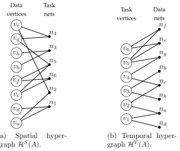
Data vertices Task nets va vd ve vf vb vh vg vc n1 n2 n6 n5 n3 n4

(a) Spatial hyper-graphHS_(A). Task vertices Data nets v1 v2 v3 v4 v5 v6 nd na nh nc nb ng ne nf (b) Temporal hyper-graphHT_(A).

Figure 4.3: Spatial and temporal hypergraphs models of sparse matrix A.

4.1.2

Spatial Hypergraph (SH)

Model Definition

For a sparse matrix A, the access of x-vector entries by different inner-product tasks can be modeled as a hypergraph model _HS_{(A) = (V}D_,NT_).

The vertex set of _HS _{consists of data vertices where each column c}

j of A

necessitates a vertex vj ∈ VD. The nets set of HS consists of task nets where

each row rj of A necessitates a net ni ∈ NT. Net nj connects data vertices

corresponding to columns that have nonzeros in row ri. That is,

P ins(nT_i ) =_{vjD : ai,j 6= 0}.

The nets and vertices in this model are associated with unit weights. This model is previously proposed in [18].

Figure 4.3a shows _HS _{model of the sample matrix A and taking net n} 5 as

an example, we can see that it connects data vertices ve, vf and vg because the

inner-product task associated with row r5 requires the x-vector entries xe, xf and

vc vg ve vf va vd vb vh n1 n2 n6 n5 n3 n4 P1 P2 P3 P4

(a) 4-way partitioning ofHS_(A).

ˆ A c g e f a d b h 1 2 3 4 5 6 × × × × × × × × × × × × × P1 P2 P3 P4 (b) Reordered matrix ˆA.

Figure 4.4: Four-way partition Π(_VD) of the spatial hypergraph given in Fig-ure 4.3a and matrix ˆA, which is obtained via reordering matrix A according to this partition.

Validity Assessment

The cut nets in a K-way partition Π(_VD_{) ofH}S _{can be used to model the number}

of cache misses that occur during the irregular access of x-vector due to loss of spatial locality, so minimizing the cutnets according to Eq. 2.3 corresponds to minimizing the number of cache misses.

A proof can be given as follows: Under the same assumptions mentioned in the proof of the SG model in the previous section, a cut net ni means that the

inner-product task corresponding to row i might not reuse the x-vector entries corresponding to vertices connected by ni in different |con(ni)| parts.

An uncut net ni tells us that the x-vector entries corresponding to vertices

connected by net niwill be reused during the inner-product task that corresponds

to row ri since they are reordered consecutively.

Figure 4.4 shows a four-way partition of _HS_{(A) model of the sample matrix}

given in Figure 4.1 and the permuted matrix ˆA. Note that row order of ˆA matrix is kept as the original order.

Figure 4.5: Temporal graph _GT_(A). Task vertices v1 v2 v3 v4 v5 v6 1 1 1 2

4.2

Exploiting Temporal Locality

In this section, we present graph and hypergraph partitioning models used in dif-ferent methods in order to exploit temporal locality in parallel SpMV. Exploiting temporal locality in CSR-based SpMV requires the alignment of rows with sim-ilar sparsity pattern, which can be encoded as the pattern of accessing x-vector entires, next to each other.

4.2.1

Temporal Graph (TG)

Model Definition

For a matrix A, the similarities between inner product tasks (rows) in terms of their access pattern to the x-vector (number of shared columns) can be modeled as a graph_GT_{(A) = (V}D_{,E) which can be called a similarity graph since it encodes}

the similarities between rows. Here an hereafter, the subscript “T” in the graph notion refers to temporal locality. The graph model_GT _{is constructed as follows,}

for each row ri of the matrix A, there exists a “task” vertex vi ∈ V. There exists

an edge ei,j ∈ E between task vertices vi and vj if the rows corresponding to

those vertices, i.e., ri and rj, have nonzeros in at least one column in common.

columns between between rows ci and cj. That is,

w(ei,j) =|{k : ak,i6= 0 ∧ ak,j 6= 0}|.

Figure 4.5 shows _GT _{model of the sample matrix given in Figure 4.1.}

Validity Assessment

The cut edges in a K-way partition Π(_VD) of _GT can be used to model the number of cache misses that occur during the irregular access of x-vector due to loss of temporal locality, so minimizing the cutsize as in Eq. 2.2 corresponds to minimizing the number of cache misses. A proof can be given as follows: Under the following assumptions:

• The cache can fit only for x-vector entries that are used during processing tasks in the same part.

• The cache line accommodates only one word.

• The rows corresponding to the vertices in a part are reordered consecutively. A cut edge ei,j will incur at most w(ei,j) extra cache misses because during the

inner-products corresponding to rows ri and rj, the w(ei,j) x-vector entries used

by tasks ti and tj may not be reused due to loss of temporal locality since the

rows ri and rj are not reordered next to each other. An uncut edge eh,` with

weight w(eh,`) means that the w(ei,j) x-vector entries used by both ti and tj will

probably be reused since rows ri and rj are reordered consecutively.

4.2.2

Temporal Hypergraph (TH)

Model Definition

For a sparse matrix A, inner-product tasks (rows) requirement of differ-ent x-vector differ-entries (columns) can be modeled as a hypergraph model

HS_{(A) = (V}D_,NT_).

The vertex set of_HS _{consists of task vertices where each row r}

iof A necessitates

a vertex vi ∈ VD. The nets set of HS consists of data nets where each column cj

of A necessitates a net nj ∈ NT. Net nj connects task vertices corresponding to

rows that have nonzeros in column cj. That is,

P ins(nD_j ) = _{viT : ai,j 6= 0}.

In other words, net nj encodes the fact that x-vector entry xj corresponding to

column cj will be accessed during the inner products of |P ins(nDj )| tasks in the

task vertex set P ins(nD

j ). In this model, we associate vertices and nets with unit

weights. This model is previously proposed in [11]. Figure 4.3b shows_HT model of the sample matrix given in Figure 4.1.

Validity Assessment

The cut nets in a K-way partition Π(_VD_{) ofH}T _{can be used to model the number}

of cache misses that occur during the irregular access of x-vector due to loss of temporal locality, so minimizing the cutnets according to Eq. 2.3 corresponds to minimizing the number of cache misses.

A proof can be given as follows: Under the same assumptions list used in the proof of _GT _{model, a cut net n}

j will incur at most most |P ins(nj)| extra cache

misses because during the inner-products in P ins(nj), the x-vector entry xj used

by those tasks may not be reused due to loss of temporal locality.

An uncut net nj tells us that the x-vector entry xj will be reused during the

inner-product task in P ins(nj) since the rows corresponding to those tasks are

Chapter 5

2D Locality Exploiting Methods

In Chapter 4, we discuss the proposed methods for reordering either rows or columns to exploit spatial or temporal localities, respectively. In this chapter, we propose methods and models to exploit spatial and temporal localities by reorder-ing rows and columns in two-dimensional manner. This chapter is organized as follows: first section presents heuristics-based reordering of rows/ columns which follows a 1D method from the previous chapter in order to reorder the dimen-sion that has not been reordered by the 1D method. In section 2 we propose a spatiotemporal bipartite graph model and a hypergraph model which can be partitioned in one phase to obtain a reordering on both rows and columns. Fi-nally in section 3 we present a two-phase method in which we reorder the sparse matrix to exploit spatial locality in the first phase and use the reordered matrix to exploit temporal locality in the second phase.

5.1

Using Heuristics with 1D Methods

Reordering methods in Chapter 4 target the exploitation of either spatial or temporal locality. In this section, we target the reordering of the dimension of the matrix (rows or columns) that had not been reordered after a 1D reordering

method from chapter 4 is applied.

Given a K-way partition Π on one dimension of the sparse matrix A, i.e., using either spatial or temporal models, in this section we show how to obtain a heuristic-based K-way partition ˆΠ on the other dimension of the sparse matrix in linear time.

Algorithm 4 Temporally-improved Spatial Reordering

Require: K-way partition vector on columns CP artvec, Reordered Matrix ˆA

tmpBuf [K] _{← ∅}

RP artvec← ∅

ptmp _{← 0}

for each row ri in ˆA do

for all column cj have nonzero in ri do

ptmp _{← CP art}vect[cj]

tmpBuf [ptmp] _{← tmpBuf[ptmp] + 1} end for

RP artvec[ri]← maxIndex(tmpBuf)

tmpBuf [K]_{← ∅} end for

return RP artvec

5.1.1

Temporally-Improved Spatial Methods (SG-H,

SH-H)

Using a spatial method from Chapter 4 (Graph or Hypergraph based), we obtain a reordering on columns (data vertices) of sparse matrix A. From this reordering, we can derive a heuristic-based reordering for rows (task vertices) of sparse matrix A to further improve the temporal locality of the matrix.

Given a K-way partition Π on the columns of the sparse matrix A, a heuristic-based K-way partition ˆΠ on the rows of the sparse matrix is obtained, in linear time, as follows: for row ri in a reordered matrix ˆA, assign ri to the part ˆPk of

ˆ

Π corresponds to part _Pk of Π which minimizes the external connections of ri

to other parts, i.e., assign ri to the part ˆPk of ˆΠ corresponds to part Pk of Π

how to obtain heuristic-based partitioning vector on rows of matrix A given a partition on columns and a reordered matrix. In this algorithm, RP artvec with

size equal to number of rows of matrix A is used to save the part number of row ri as RP artvec[i], CP artvec with size equal to number of columns of matrix A is

used for columns assignment to parts as in RPvec, and tmpBuf that has a size

equal to number of parts K is used as a buffer during processing row ri to know

how many columns connected with ri are in each part.

5.1.2

Spatially-Improved Temporal Methods (TG-H,

TH-H)

Using a temporal method from Chapter 4 (Graph or Hypergraph based), we ob-tain a reordering on rows (task vertices) of sparse matrix A. Form this reordering, we can derive a heuristic-based reordering for columns (data vertices) of sparse matrix A to further improve the spatial locality of the matrix.

The problem definition and details of the method are similar to the previous section with changing the roles of rows and columns.

Algorithm 5 shows how to obtain a heuristic-based partitioning vector on columns of matrix A given a partition on rows and a reordered matrix. In this algorithm, CP artvec with size equal to number of columns of matrix A is used to

save the part number of column cj as CP artvec[j], RP artvec with size equal to

number of rows of matrix A is used for rows assignment to parts as in CP artvec,

and tmpBuf that has a size equal to number of parts K is used as a buffer during processing column cj to know how many rows connected with cj are in each part.

Note that this algorithm processes the nonezeros in column-major order, i.e. it uses CCS scheme to store the sparse matrix.

Algorithm 5 Spatially-improved temporal Reordering

Require: K-way partition vector on rows RP artvec, Reordered Matrix ˆA

tmpBuf [K] _{← ∅}

CP artvec ← ∅

ptmp _{← 0}

for each column cj in ˆA do

for all row ri have nonzero in cj do

ptmp _{← RP art}vect[ri]

tmpBuf [ptmp] _{← tmpBuf[ptmp] + 1} end for

CP artvec[cj]← maxIndex(tmpBuf)

tmpBuf [K]_{← ∅} end for

return CP artvec

5.2

Simultaneous Methods

In this section, we propose a bipartite graph partitioning model called STG and a hypergraph partitioning model called STH in order to encode spatial and tem-poral localities simultaneously.

5.2.1

Bipartite Spatiotemporal Graph (STG)

Model Definition

For a matrix A, the mutual requirement between the x-vector entries and the inner product tasks can be modeled as a bipartite graph _GST_{(A) = (V = V}D_{∪ V}T_,E).

The vertex set of _GST _{consists of data vertices and task vertices as follows: each}

row ri of the sample matrix necessitates a task vertex vi ∈ VT and each column

cj necessitates a data vertex vj ∈ VD. There is an edge ei,j between vertex vi and

vj if there is a nonezero ai,j between row ri and column cj. We associate unit

Data vertices Task vertices va vb vc vd ve vf vg vh v1 v2 v3 v4 v5 v6

Figure 5.1: Bipartite Graph model _GST_{(A) for exploiting spatial and temporal}

localities simultaneously.

Figure 5.1 shows the bipartite _GST _{model of the sample matrix given in}

Fig-ure 4.1. In the figFig-ure, the edges show the mutual requirements of the task vertices to the data vertices and vice versa.

Validity Assessment

The cut edges in a K-way partition Π(_{V) of G}ST _{can be used to model the number}

of cache misses that occur during the irregular access of x-vector due to loss of spatial and temporal localities, so minimizing the cutsize as in Eq. 2.2 corresponds to minimizing the number of cache misses.

A proof can be given as follows: Under the following assumptions:

• Each cache line accommodates W words. • Each part in Π(V) contains exactly W vertices.

• The cache can fit only for x-vector entries that are used during processing tasks in the same part.

• Columns correspond to vertices in a part are reordered consecutively. • Rows correspond to vertices in a part are reordered consecutively.

A cut edge ei,j that connects task vertex vi and data vertex vj means two things:

1. The inner-product task ti will not reuse the line contains data element xj

due to loss of spatial locality.

2. Data element xj will not be reused by the inner-product task ti due to loss

of temporal locality.

While an uncut edge means the opposite, this proof does not cover the relation among tasks or among data entries. There is an indirect relation between task vertices that goes through data vertices as follows: minimizing the cut edges means clustering a task vT_i with the data vertices it will use, i.e, the set Adj(v_iT), in the same part. This will encourage the task vT_j with_{Adj(viT)_{∩ Adj(vj}T)_{} 6= ∅} to be in the same part to decrease the cut edges during the K-way partitioning Π(_V).

5.2.2

Spatiotemporal Hypergraph (STH)

Model Definition

For a matrix A, the mutual requirement between the x-vector entries and the inner product tasks can be modeled as a hypergraph model HST_{(A) = (V = V}D _{∪ V}T_{,N = N}T _{∪ N}D_).

The vertex set of _HST consists of data vertices and task vertices as follows: each row ri of the sample matrix necessitates a task vertex vi ∈ VT and each

column cj necessitates a data vertex vj ∈ VD. The net set of HST consists of

data nets and task nets as follows: each row ri of the sample matrix necessitates

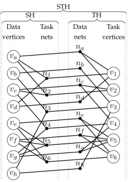
SH STH TH Data vertices Task nets Data nets Task vertices va na vb nb vc nc vd nd ve ne vf nf vg ng vh nh v1 n1 v2 n2 v3 n3 v4 n4 v5 n5 v6 n6

Figure 5.2: Hypergraph model_HST_{(A) for exploiting spatial and temporal}

local-ities simultaneously.

HST_{(A) models the dependencies between task and data vertices as follows: a}

task net nT_i connects data vertices corresponding to columns that have nonzeros in row ri. It also has one more connection to vertex vi which corresponds to row

ri. Data net nDj connects task vertices corresponding to rows that have nonzeros

in column cj. It also connects vertex vj which corresponds to column cj. That is,

P ins(nD_j ) = _{vT_i : ai,j 6= 0} ∪ {vDj }.

P ins(nT_i ) = _{vD_j : ai,j 6= 0} ∪ {viT}. (5.1)

We associate unit weights with all nets and all vertices.

Figure 5.2 shows_HST _{model of the sample matrix given in Figure 4.1. As seen}

in the figure, the _HST _{model is build using both H}S _{and H}T _{models with the}

Validity Assessment

The cut nets in a K-way partition Π(_{V) of H}ST _{can be used to model the number}

of cache misses that occur during the irregular access of x-vector due to loss of spatial and temporal localities, so minimizing the cutnets according to Eq. 2.3 corresponds to minimizing the number of cache misses.

A proof can be given as follows: Under the same assumptions used in the proof of the _GST _{model in the previous section, a data cut net n}D

j means that x-vector

entry xj will not be re-used by, at most, |con(nDj )| − 1 tasks because the rows

corresponding to the tasks are not ordered near each other. A data uncut net nD_j means the opposite because the tasks are reordered consecutively. Similarly, a task cut net nT_i means that the corresponding task ti will not reuse the lines

that contain x-vector entries that correspond to data vertices in P ins(ni). A

task uncut net nT

i means the opposite since the columns corresponding to data

vertices are reordered consecutively.

5.2.3

Spatially-biased Spatiotemporal Hypergraph (S

TH)

For a sample matrix A, the mutual requirement between the x-vector entries (columns) and the inner product tasks (rows) can be modeled as a hypergraph model _HS2T_{(A) = (V = V}D_{∪ V}T_{,N = N}T_).

The vertex set of _HS2_T

consists of data vertices and task vertices as follows: each row ri of the sample matrix necessitates a task vertex vi ∈ VT and each

column cj necessitates a data vertex vj ∈ VD. The net set ofHST consists of task

nets where each row ri of the sample matrix necessitates a task net ni ∈ NT.

HS2_T

(A) models the dependencies between task and data vertices as follows: a task net nT

i connects data vertices corresponding to columns that have nonzeros

Data vertices Task nets Task vertices va vb vc vd ve vf vg vh v1 n1 v2 n2 v3 n3 v4 n4 v5 n5 v6 n6

Figure 5.3: Hypergraph model _HS2_T

(A) for exploiting spatial and temporal lo-calities simultaneously.

ri. That is,

P ins(nT_i ) = _{vjD : ai,j 6= 0} ∪ {viT}. (5.2)

We associate unit weights with all nets and all vertices. Figure 5.3 shows the _HS2_T

model of the sample matrix given in Figure 4.1. In the figure, the task net n5 connects data vertices ve, vf and vg because the inner

product task associated with row r5 requires the x-vector entries xe, xf and xg.

Net n5 also connects v5.

This models can be seen as a variation of the _HST _{model where the set of}

vertices to be partitioned is preserved while the number of nets is decreased by C, which is number of columns of matrix A, and the total number of pins is decreased by nnz + R, which is the number of nonzeros and the rows of the matrix A, respectively.

A task net ni connecting vertices in the vertex set P ins(ni) encodes the

re-quirement of x-vector entries in_{xk : vk ∈ P ins(ni)\ {vi}} by the inner product

common parts increases the possibility of exploiting spatial locality in accessing x-vector entries during the inner-product task ti Since task vertex vi is connected

with task net ni, minimizing the cut nets during the k-way partition ofHS 2_T

mo-tivates vi to be clustered in the part that its corresponding task net ni connects

most. This relation does not improve temporal locality with this direct defini-tion, however there is an indirect relation between task vertices which states the following: if both nets ni, nj ∈ NT have maximum number of pins in part Pk,

then clustering task vertices vi and vj toPkwill imporve the temporal locality of

vi and vj in accessing x-vector entries corresponding to data vertices in part Pk.

HS2_T

model encodes the exploitation of spatial locality as a primary parti-tioning goal, while it exploits temporal locality as a secondary goal. It is very similar to the heuristic-based Temporally-improved spatial hypergraph described in Section 5.1.1.

5.2.4

Temporally-biased Spatiotemporal Hypergraph (ST

H)

For a matrix A, the mutual requirement between the x-vector entries (columns) and the inner product tasks (rows) can be modeled as a hypergraph model HST2_{(A) = (V = V}D _{∪ V}T_{,N = N}D_).

The vertex set of _HST2

consists of data vertices and task vertices as follows: each row ri of the sample matrix necessitates a task vertex vi ∈ VT and each

column cj necessitates a data vertex vj ∈ VD. The net set of HST 2

consists of data nets where each column cj of the sample matrix necessitates a data net

nj ∈ ND.

HST2

(A) models the dependencies between task and data vertices as follows: a data net nD_j connects task vertices corresponding to rows that have nonzeros in column cj. It also connects vertex vj which corresponds to column cj. That is,

P ins(nD_j ) =_{vT_i : ai,j 6= 0} ∪ {vDj }. (5.3)

model of the sample matrix given in Figure 4.1.

This model can be seen as a variation of the _HST _{model where the set of}

vertices to be partitioned is preserved while the number of nets is decreased by R, which is number of columns of matrix A, and the total number of pins is decreased by nnz + C, which are the number of nonzeros and the columns of the matrix A, respectively.

A data net nj connecting vertices in the vertex set P ins(nj) encodes the access

of the inner-products corresponding of rows in _{rk : vk ∈ P ins(nj)\ {vj}} to

x-vector entry xj. Hence, clustering vertices in P ins(nj)\ {vj} into common parts

increases the possibility of exploiting temporal locality in accessing xj. Since data

vertex vj is connected with data net nj, minimizing the cut nets during the k-way

partition of _HST2

motivates vj to be clustered in the part that its corresponding

data net nj connects most. This relation does not improve spatial locality with

this direct definition, however there is an indirect relation between data vertices which states the following: if both nets ni, nj ∈ ND have maximum number

of pins in part _Pk, then clustering data vertices vi and vj to Pk will improve

the spatial locality of vi and vj since task vertices in part Pk will access them,

probably, together. HST2

model encodes the exploitation of temporal locality as a primary par-titioning goal, while it exploits spatial locality as a secondary goal. It is very similar to the heuristic-based Spatially-improved temporal hypergraph described in Section 5.1.2.

5.3

Two-Phase Methods

The graph and hypergraph models proposed previously are based on the assump-tion that each cache miss brings one data word to the cache. Given the fact that each cache miss brings a cache line, consists of W words, we can observe that this fact is useful mostly in spatial locality and it can be utilized for further

Data vertices Data nets Task vertices va na vb nb vc nc vd nd ve ne vf nf vg ng vh nh v1 v2 v3 v4 v5 v6

Figure 5.4: Hypergraph model _HST2

(A) for exploiting spatial and temporal lo-calities simultaneously.

improvement in building the models. In this section we propose two-phase meth-ods that uses two 1D methmeth-ods from Chapter 4 to exploit spatial and temporal localities. The two-phase methods has to exploit spatial locality in the first phase then temporal locality in the second. In the first phase, a spatial graph or hyper-graph method is applied to the sparse matrix in order to reorder its columns and exploit spatial locality. This reordering, which corresponds to reordering x-vector entries, is used to determine the allocation of x-vector entries to blocks of size W as follows: the first W x-vector entries go to the first block, the second W entries go to the second block ... etc. In the second phase, we utilize a temporal method with column stripes, which correspond to x-vector blocks, treated as data vertices/ nets instead of a single column for each vertex/ net.

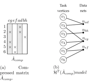
ˆ Acomp cg ef ad bh 1 2 3 4 5 6 × × × × × × × × (a) Com-pressed matrix ˆ Acomp. Task vertices Data nets v6 v5 v4 v3 v2 v1 nef ncg nbh nad (b) HT_{( ˆA} comp)model

Figure 5.5: Compressed matrix ˆAcomp after the first phase of the Two-phase

method and the _HT model representation of ˆAcomp

5.3.1

Two-Phases Hypergraph method (SH

_→TH

)

First Phase

For a matrix A, consider the 1D hypergraph model_HS_{(A) = (V}D_,NT_{) and its}

K-way partition Π(_VD_{). Using the K-way partitioning, we can reorder the columns}

of the matrix as describes in Section 4.1.2. The reordered matrix, i.e., output of the SH method, is referred to as ˆA. The same reordering vector used to reorder the columns of matrix A is used to reorder the entries of the x-vector. Following the reordering, we perform a compression on the columns of the reordered matrix

ˆ

A of size m_{× n as follows: take the first W columns and pack them in one} column where in each row of this column, there exists a nonzero element if, for row ri and column stripe α, {Sα.W +W_{j=α.W +1}ai,j} 6= ∅. Then take the second, third

... etc. where the last set of columns might have a length less than W , that is, (W _{− δ) : 0 ≤ δ ≤ W . The resulting compressed matrix is called ˆ}Acomp which

has a size of m_{× ˆn, where ˆn = dW}n_{e is the actual number of cache lines will be} brought to the cache during the inner-product task ri.

Second Phase

For the compressed matrix ˆAcomp, we can use the temporal hypregraph model

described in Section 4.2.2 to model the requirement of the inner-product tasks to the x-vector blocks. Figure 5.5 shows the compressed matrix ˆAcomp and the

temporal hypergraph model representation of ˆAcomp.

5.3.2

Two-Phases Graph method (SG

_→TG

)

This method is similar to the previous method but it uses graph-based models instead of hypergraph-based models.

In the first phase, we use the spatial graph model_GS _{described in Section 2.1.1}

to obtain a K-way partition Π(_VD) to reorder the columns of the sparse matrix A. Using the partition and following the same steps in the previous section, we obtain the compressed matrix ˆAcomp. In the second phase, we use the temporal

graph model_GT _{based on the compressed matrix ˆA}

compto model the requirement

Chapter 6

Experiments

6.1

Data Set

We test the validity of the proposed methods on a set of sparse matrices with irregular sparsity patterns from different applications. All the matrices are ob-tained from University of Florida Sparse Matrix Collection [22]. Table 6.1 shows the properties of the test matrices, including “avg” and “max” which respectively means the average and maximum number of nonzeros per row/column. The “cov” means the coefficient of variation of the number of nonzeros per row/column. The matrices in the table are grouped into three categories: Symmetric, Non-symmetric Square and Rectangular.

6.2

Experimental Framework

The performances of the proposed methods are evaluated on a single 60-core Xeon Phi 5110 co-processor which runs 4 hardware threads per core and has 512KB L2 cache per core. We use the Sparse Library (SL) [23, 19, 24], which is highly optimized for SpMV operations on Xeon Phi co-processors, to perform our

tests. The SL library has many methods to perform SpMV, we use the method which reported to perform best [23] on Xeon Phi which is Row-Distributed Hilbert Scheme (RDHilbert). This method uses vectorized Bidirectional Incremental CRS (vecBICRS) as a data structure to store the sparse matrix and algorithm to perform the SpMV tasks. We use 240 threads, which is number of all threads in all cores, as suggested in [23, 24]. Yzelman has introduced the explicitly vectorized SpMV in [23] which shows a considerable improvement on the running time with Xeon Phi co-processors. The vectorization options, which yzelman also call blocking options, can be any combination of two numbers if multiplied their product is number of double precision operations that the Vector Processing Unit (VPU) can perform per cycle in the Xeon Phi, i.e., if the vector size is 8, the blocking options can be 1_{× 8, 2 × 4, 4 × 2 and 8 × 1. There is also an additional} blocking option 1_{× 1 which means no vectorization. The aforementioned method} in SL library has been slightly modified by removing the Space Filling Curve algorithm (Hilbert’s Curves) since it might affect the reordering obtained by the proposed methods. We use this modified algorithm to test all methods and as a baseline algorithm, which is referred to throughout this chapter as BL.

To obtain a K-way partitioning on the graph and hypergraph models we use MeTiS [5] and PaToH [7, 25] respectively.

MeTiS is used as a multilevel K-way partitioner with the partitioning objec-tive of minimizing the cut edge cost as in Eq. 2.2. PaToH is also used as a K-way partitioner with the partitioning objective of minimizing the “Connectivity-1” cost according to Eq. 2.3. MeTiS and PaToH are used with default parameters with the exception of the allowed imbalance ratio, which is set to 30% because we focus more on reordering than load balancing. Since these tools contain random-ized algorithms, we repeat each partitioning instance three times and report the average results. While partitioning graph and hypergraph models, K is selected such that each part is sufficiently small to obtain cache-oblivious reorderings. That is, each matrix’s storage size (in terms of KB), which is reported by the SL library, is divided by 32KB to obtain K.

6.3

Performance Evaluation

In this section, we evaluate the performances of the proposed methods accord-ing to their performance speed in Gflop/s. The evaluation process consists of three main parts as follows: first we compare Graph vs Hypergraph partitioning methods, then we compare separate methods with simultaneous methods and af-terwards we show the importance of exploiting locality and how it boosts up the effectiveness of vectorization. We use performance profiles to compare different methods. The performance profiles compare different methods by showing the fraction of test cases for how much each method is close to the best. In other words, if a method reaches 100% of test cases with full closeness to the best, i.e. 1, that means this method performs best in all test cases. Tables 6.3 is used to show the geometric means of the proposed methods for all possible vectorization options. In the table, “Best” means the geometric mean of all performances per matrix that performed best among all blocking options. Also, vec.Avg. means the geometric mean of all average performances among all blocking options, except for 1_{× 1, per matrix.}

6.3.1

Graph vs Hypergraph Partitioning Methods

Here we compare the performances of graph-based and hypergraph-based meth-ods.

Figure 6.1 shows the performance profiles of the SpMV times for all 1D and 2D methods, except for the hypergraph-based methods in Sections 5.2.3 and 5.2.4 because they do not have equivalent graph methods. As seen in the figure, the HP-based methods perform significantly better than the GP-based methods. However, in terms of temporal methods, the difference become smaller since tem-poral locality is less sensitive to the deficiencies of the graph models described in [25].

0.0 0.1 0.2 0.3 0.4 0.5 0.6 0.7 0.8 0.9 1.0 1.0 1.05 1.1 1.15 1.2

Fraction of test cases

Parallel SpMV time relative to the best SH SG

(a) Spatial Methods

0.0 0.1 0.2 0.3 0.4 0.5 0.6 0.7 0.8 0.9 1.0 1.0 1.05 1.1 1.15 1.2

Fraction of test cases

Parallel SpMV time relative to the best TH TG (b) Temporal Methods 0.0 0.1 0.2 0.3 0.4 0.5 0.6 0.7 0.8 0.9 1.0 1.0 1.05 1.1 1.15 1.2

Fraction of test cases

Parallel SpMV time relative to the best SH-H SG-H

(c) Huristic-based Spatial Methods

0.0 0.1 0.2 0.3 0.4 0.5 0.6 0.7 0.8 0.9 1.0 1.0 1.05 1.1 1.15 1.2

Fraction of test cases

Parallel SpMV time relative to the best TH-H TG-H

(d) Huristic-based Temporal Methods

0.0 0.1 0.2 0.3 0.4 0.5 0.6 0.7 0.8 0.9 1.0 1.0 1.05 1.1 1.15 1.2

Fraction of test cases

Parallel SpMV time relative to the best STH STG

(e) Spatiotemporal Methods

0.0 0.1 0.2 0.3 0.4 0.5 0.6 0.7 0.8 0.9 1.0 1.0 1.05 1.1 1.15 1.2

Fraction of test cases

Parallel SpMV time relative to the best SH+THline SG+TGline

(f) TwoPhase Methods Figure 6.1: Performance profiles for HP-based methods vs GP-based methods.

6.3.2

Reordering with two 1D methods vs simultaneous

methods

Fraction of test cases

Parallel SpMV time relative to the best

STG SG+TG (a) GP Methods 0.0 0.1 0.2 0.3 0.4 0.5 0.6 0.7 0.8 0.9 1.0 1.0 1.05 1.1 1.15 1.2 1.25

Fraction of test cases

Parallel SpMV time relative to the best

STH SH+TH

(b) HP Methods

Figure 6.2: Performance profiles for separate vs simultaneous graph and hyper-graph partitioning methods.

A possible straight forward method to utilize 1D models in 2D reordering is to apply spatial method to reorder the columns of the sparse matrix and a temporal method to reorder the rows of the sparse matrix. Though we have four possible combinations by mixing graph and hypergraph models, we consider 1D graph models together and hypergraph models together. These methods are called SG+TG and SH+TH, respectively. Note that in SG+TG and SH+TH we apply each method separately and independently. In this section, we compare the above mentioned methods with 2D methods that target the exploitation of spatial and temporal localities simultaneously.

Figure 6.2 shows the performance profiles that compare the SpMV times of separate 2D reordering vs simultaneous 2D reordering. The figure shows how

simultaneous methods perform significantly better than separate methods. How-ever, SG+TG and SH+TH can be useful if used to reorder symmetric matrices. Table 6.4 shows the geometric means of all matrices per category. In symmetric category, its obvious that SG+TG and SH+TH perform close to the simultaneous graph and hypergraph methods, respectively, while in other categories simultan-ious methods perform considerably better. The reason behind this is that in symmetric matrices both spatial and temporal models are the same so utilizing them to exploit both localities is nearly equal to using simultaneous methods.

6.3.3

Comparison of 2D Methods

Fraction of test cases

Parallel SpMV time relative to the best

STH S2TH ST2H SH+THline TH-H SH-H

Figure 6.3: Performance profiles for comparing the performances of hypergraph-based 2D methods.

In this section, we compare the 2D methods and study the benefits of using each one of them. We exclude the graph-based methods from this section because we have already shown that hypergraph-based methods perform much better than the graph-based methods. Figure 6.3 shows the performance profiles that compare

the SpMV times of 2D hypergraph based methods. As seen in the figure, as well as in Table 6.3, STH outperform all other methods and it is the best fit for all vectorization options.

Figure 6.3 also shows that the other 2D hypergraph-based methods have a comparable performance. Table 6.3 shows that the geomeans of SH-H, TH-H, S2_{TH, ST}2_{H and SH→TH}

linemethods are close to each other. We can

distin-guish between the 2D methods in Table 6.6 by their number of best instances. ST2_{H method is the second best, after STH, with 13 instances out of 53. The}

methods ST2H and TH-H both follow the same logic, in TH-H the temporal locality is improved first by reordering rows using TH method, then according to the reordered matrix we reorder the columns in a way that best fits the new temporally-improved matrix as discussed in Section 5.1.2. ST2_{H does something}

similar during the partitioning of _HST2

model, it encourages a data vertex to be clustered to the part that connects its corresponding data net most, in order to minimize the cut nets. The main difference between ST2H and TH-H is the load balancing on the secondary exploiting objective. In ST2H, clustering data ver-tices to parts is done during the partitioning of the model so the load balancing criteria holds. However in TH-H, the clustering of data vertices is done separately and it does not consider any load balancing criteria. Note that the same compar-ison terms are applicable on the comparcompar-ison between SH-H and S2_{TH. Table 6.5}

shows the number of vertices, nets and pins in every hypergraph partitioning model. Number of pins in this context means the total number of connections between nets and vertices. Note that m is number of rows in the matrix and n is the number of columns.

Table 6.5: Number of vertices, nets and pins for the 2D models Method # vertices # nets # pins

SH-H n m nnz TH-H m n nnz S2_{TH m+n n n + nnz} ST2_{H m+n m m + nnz} STH m+n m+n m+n+2nnz THline φ 1 n m nnz THline φ 2 m n nnz

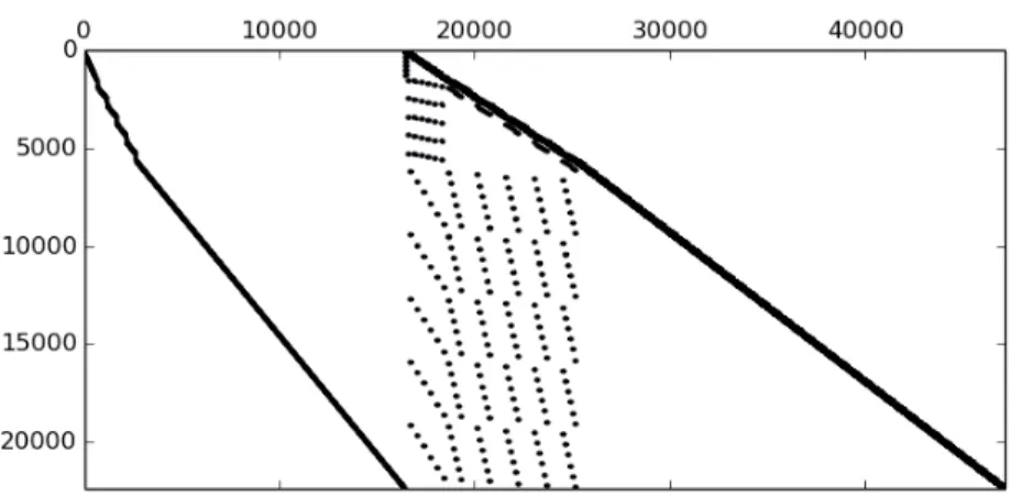
(a) 144 (b) 144 after STH

(c) delaunay n18 (d) delaunay n18 after STH

(e) pds-80

(f) pds-80 after STH

Figure 6.4: Plots of sample matrices before and after applying STH reordering method.