ITu1E.1.pdf Imaging and Applied Optics © OSA 2013
Degrees of freedom of optical systems and signals
with applications to sampling and system simulation
Figen S. Oktem1,∗and Haldun M. Ozaktas2
1Department of Electrical and Computer Engineering,
University of Illinois at Urbana-Champaign, Urbana, Illinois 61801, USA
2Department of Electrical Engineering, Bilkent University, TR-06800 Bilkent, Ankara, Turkey
Abstract: We study the degrees of freedom of optical systems and signals based on space-frequency (phase space) analysis. At the heart of this study is the relationship of the linear canonical transform domains to the space-frequency plane. Based on this relationship, we discuss how to explicitly quantify the degrees of freedom of first-order optical systems with multiple apertures, and give conditions for lossless transfer. Moreover, we focus on the degrees of freedom of signals in relation to the space-frequency support and provide a sub-Nyquist sampling approach to represent signals with arbitrary space-frequency support. Implications for simulating optical systems are also discussed.
© 2013 Optical Society of America
1. Introduction
Optical systems involving thin lenses, sections of free space in the Fresnel approximation, sections of quadratic graded-index media, and arbitrary combinations of any number of these are referred to as first-order optical systems or quadratic-phase systems. Mathematically, such systems can be modeled as linear canonical transforms (LCTs), which form a three-parameter family of integral transforms [1–6]. The output light field fM(u) of a quadratic-phase system
is related to its input field f(u) through [1, 2]
fM(u) ≡ (CMf)(u) ≡ Z ∞ −∞ CM(u, u′) f (u′) du′, CM(u, u′) ≡ r 1 Be −iπ/4eiπ(D Bu2−21Buu′+ABu′2), (1)
for B6= 0, where CM is the unitary LCT operator with parameter matrix M= [A B; C D] with AD − BC = 1. The
transform matrix M is useful in the analysis of optical systems because if several systems are cascaded, the overall system matrix can be found by multiplying the corresponding matrices. The LCT family includes the Fourier and fractional Fourier transforms, coordinate scaling, chirp multiplication and convolution operations as its special cases.
The ath-order fractional Fourier transform (FRT) [1] of a function f(u), denoted by fa(u), is commonly defined as
fa(u) ≡
Z ∞ −∞
Ka(u, u′) f (u′) du′, Ka(u, u′) ≡ Aφeiπ(cotφ u
2−2 csc φ uu′+cot φ u′2
), Aφ=p1− i cotφ, φ= aπ/2, (2) when a6= 2 j and Ka(u, u′) =δ(u − u′) when a = 4 j and Ka(u, u′) =δ(u + u′) when a = 4 j ± 2, where j is an integer.
2. Equivalence of linear canonical transform domains to oblique axes in the space-frequency plane
It is well known that the ath order fractional Fourier transform domain is an oblique axis in the space-frequency plane [1, 7]. It has been recently shown that LCT domains are equivalent to scaled FRT domains and thus to scaled oblique axes in the space-frequency plane [8]. The equivalence between LCT and FRT domains is based on expressing the LCT as a chirp-multiplied and scaled FRT. Multiplication is not considered to be an operation that changes the domain of a signal, and scaling of the axis is a relatively trivial modification of a domain. Therefore, the only part of the LCT operation that genuinely corresponds to a domain change is the FRT in it, and the linear canonical transformed signal essentially lives in a scaled FRT domain, and hence in a scaled oblique axis in the space-frequency plane.
Based on this many-to-one association of LCTs with FRTs, LCT domains can be labeled and monotonically ordered by an associated fractional order parameter, instead of their usual three parameters, which do not directly lend themselves to a natural ordering. This has important implications for optical systems modeled by LCTs. The optical amplitude distribution at any plane along the optical axis can be expressed as a three-parameter LCT of the input.
ITu1E.1.pdf Imaging and Applied Optics © OSA 2013
Being able to associate a single monotonically increasing parameter with each location along the optical axis offers a vastly more transparent understanding of the evolution of the optical amplitude distribution, as opposed to imagining that the light goes through an unidentified and unsequenced series of three-parameter domains whose whereabouts we cannot visualize. This interpretation of LCT domains also ties together the LCT description of such optical systems with descriptions viewing propagation as an act of continual fractional Fourier transformation.
3. The Bicanonical Width Product: a Generalization of the Space-Bandwidth Product
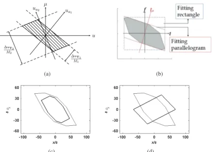
If a set of signals is highly confined to finite intervals in two arbitrary LCT domains, the space-frequency support (phase space support) is a parallelogram (see Fig. 1a). The number of degrees of freedom of this set of signals is given by the area of this parallelogram, which is equal to the bicanonical width product but usually smaller than the conventional space-bandwidth product [8].
The conventional space-bandwidth product is the minimum number of samples required to uniquely identify a signal out of all possible signals whose energies are approximately confined to given space and frequency intervals. The minimum number of samples needed to fully characterize an approximately space- and band-limited signal can also be interpreted as the number of degrees of freedom of the set of signals. More generally, the number of degrees of freedom is given by the area of the space-frequency support, regardless of its shape. When the space-frequency support is not a rectangle perpendicular to the axes, the actual number of degrees of freedom will be smaller than the space-bandwidth product of the signal. Thus, when we are confronted with a set of signals which are highly confined to finite intervals in two arbitrary LCT domains, the bicanonical width product, defined as the area of the parallelogram defined by these two extents, will be a better measure of the number of degrees of freedom of the set of signals, than the conventional space-bandwidth product. This allows us to represent and process signals with fewer samples [8].
4. Degrees of Freedom and Efficient Signal Representation
Application of the Shannon-Nyquist approach to a space-frequency support of arbitrary shape amounts to enclosing the support with a rectangle perpendicular to the space and frequency axes. The number of samples is given by the area of the rectangle and equals the space-bandwidth product, which may be considerably larger than the area of the space-frequency support and the actual number of degrees of freedom of the signals. Hence when signals do not have a rectangular space-frequency support perpendicular to the space-frequency axes, the space-bandwidth product overstates the actual number of degrees of freedom. We can represent these signals with a number of samples less than the space-bandwidth product. It may frequently be possible to more tightly enclose the actual space-frequency support with a parallelogram than with a rectangle. Then, the bicanonical width product may better represent the actual number of degrees of freedom, and we will be able to represent and reconstruct the signals with less samples than required by the Shannon-Nyquist sampling theorem. This approach reduces to a simple geometrical problem which requires to find the smallest parallelogram enclosing the space-frequency support (as an example, see Fig. 1b). The area of the parallelogram gives the number of samples needed and the reconstruction is possible through the LCT interpolation formula [9, 10] given by f(u) =δu| cscφ| ∆uMe−iπ cot φ u
2 × ∑∞
n=−∞f(nδu) sinc(cscφ∆uM(u − nδu))eiπ cot φ (n δ u) 2
.
5. Degrees of Freedom of Optical Systems and Their Simulation
By utilizing the concepts outlined in previous sections, we can explicitly determine the space-frequency window (phase space window) for optical systems consisting of an arbitrary sequence of lenses and apertures separated by arbitrary lengths of free space [11]. If the space-frequency support of a signal lies completely within this window, the signal passes without information loss (see Fig. 1c). When it does not, the parts that lie within the window pass and the parts that lie outside of the window are blocked, a result which is valid to a good degree of approximation for most systems of practical interest. Also, the maximum number of degrees of freedom that can pass through the system is given by the area of its space-frequency window. Once established, these results provide considerable insight and guidance into the behavior and design of systems involving multiple apertures. They can help us design systems in a manner that minimizes information loss. An advantage of our approach is that it does not require assumptions regarding the signals during analysis or design, since the concept of a system window is signal-independent.
The fact that all physical systems support only a finite number of degrees of freedom means that their effect on signals can be simulated accurately with discrete systems. Recent work [12, 13] showed that if the number of samples
Nis chosen to be at least equal to the bicanonical-width product of the set of signals we are dealing with, the discrete LCT (DLCT) can be used to obtain a good approximation to the continuous LCT, limited only by the fundamental fact that a signal cannot have strictly finite extent in more than one domain. The exact relation between the discrete and
ITu1E.1.pdf Imaging and Applied Optics © OSA 2013 µ u ua1 ua2 ∆uT1 M 1 ∆uT2 M2 (a) (b) (c) (d)
Fig. 1: (a) The space-frequency support (phase space support) when finite extents are specified in two LCT domains. The area of the parallelogram is equal to ∆uM1∆uM2|β1,2|, where ∆uM1 and∆uM2 are the extents of the signal in the LCT domains, M1and M2are the corresponding scales, andβ1,2is the parameter of the LCT between these two domains [8]. (b) The smallest enclosing parallelogram (solid) and rectangle (dashed), both under the constraint that the signal is sampled in the space domain t. The shaded region is the space-frequency support. (c) The signal support is wholly contained within the system window so there is no loss of information [11]. (d) The part of the signal support lying within the system window will pass, and the parts lying outside will be blocked [11].
continuous LCTs [12] precisely shows the approximation involved and demonstrates how the approximation improves with increasing N. A graphic illustration of the resulting algorithm is given in [14].
We now discuss how to optimally simulate optical systems using this definition of the DLCT when an input signal with known space-frequency support is given. The required number of samples can be found by fitting a parallelogram to the space-frequency support, such that two opposing sides are perpendicular to the x axis (the input domain) and the other sides are perpendicular to the oblique axis corresponding to the output LCT domain. The area of the smallest fitting parallelogram gives the number of samples that needs to be used for an accurate DLCT computation. Then the samples of the continuous signal at the output of the optical system can be obtained by sampling the input signal at this rate and then computing its DLCT.
H. M. Ozaktas was supported in part by the Turkish Academy of Sciences.
References
1. H. M. Ozaktas, Z. Zalevsky, and M. A. Kutay, The Fractional Fourier Transform with Applications in Optics and Signal Processing (New York: Wiley, 2001).
2. K. B. Wolf, Integral Transforms in Science and Engineering (Plenum Press, 1979).
3. A. Stern, “Sampling of linear canonical transformed signals,” Signal Process. 86, 1421–1425 (2006).
4. A. Koc, H. M. Ozaktas, C. Candan, and M. A. Kutay, “Digital computation of linear canonical transforms,” IEEE Trans. Signal Process.
56, 2383–2394 (2008).
5. F. S. Oktem, “Signal representation and recovery under partial information, redundancy, and generalized finite extent constraints,” Master’s thesis, Bilkent Univ., Turkey (2009).
6. S.-C. Pei and J.-J. Ding, “Closed-form discrete fractional and affine Fourier transforms,” IEEE Trans. Signal Process. 48, 1338–1353 (2000). 7. H. M. Ozaktas and O. Aytur, “Fractional Fourier domains,” Signal Process. 46, 119–124 (1995).
8. F. S. Oktem and H. M. Ozaktas, “Equivalence of linear canonical transform domains to fractional Fourier domains and the bicanonical width product: a generalization of the space–bandwidth product,” J. Opt. Soc. Am. A 27, 1885–1895 (2010).
9. X.-G. Xia, “On bandlimited signals with fractional Fourier transform,” IEEE Signal Process. Lett. 3, 72–74 (1996).
10. A. Zayed, “On the relationship between the Fourier and fractional Fourier transforms,” IEEE Signal Process. Lett. 3, 310–311 (1996). 11. H. M. Ozaktas and F. S. Oktem, “Phase-space window and degrees of freedom of optical systems with multiple apertures,” J. Opt. Soc. Am.
A 30, 682–690 (2013).
12. F. S. Oktem and H. M. Ozaktas, “Exact relation between continuous and discrete linear canonical transforms,” IEEE Signal Process. Lett.
16, 727–730 (2009).
13. A. Stern, “Why is the linear canonical transform so little known?” AIP Conf. Proc. 860, 225–234 (2006).
14. J. J. Healy and J. T. Sheridan, “Reevaluation of the direct method of calculating Fresnel and other linear canonical transforms,” Optics letters 35, 947–949 (2010).