Full Terms & Conditions of access and use can be found at
http://www.tandfonline.com/action/journalInformation?journalCode=tprs20
Download by: [Bilkent University] Date: 13 November 2017, At: 03:04
ISSN: 0020-7543 (Print) 1366-588X (Online) Journal homepage: http://www.tandfonline.com/loi/tprs20
Integrated scheduling and tool management in
flexible manufacturing systems
M. Selim Akturk & Serkan Ozkan
To cite this article: M. Selim Akturk & Serkan Ozkan (2001) Integrated scheduling and tool management in flexible manufacturing systems, International Journal of Production Research, 39:12, 2697-2722, DOI: 10.1080/00207540110051941
To link to this article: http://dx.doi.org/10.1080/00207540110051941
Published online: 14 Nov 2010.
Submit your article to this journal
Article views: 99
View related articles
Integrated scheduling and tool management in ¯ exible manufacturing
systems
M. SELIM AKTURK{* and SERKAN OZKAN{
A multistage algorithm is proposed that will solve the scheduling problem in a ¯ exible manufacturing system by considering the interrelated subproblems of processing time control, tool allocation and machining conditions optimization. The main objective of the proposed algorithm is to minimize total production cost consisting of tooling, operational and tardiness costs. The proposed integrated approach recognizes an important trade-oŒin automated manufacturing systems that has been largely unrecognized, and which is believed can be eŒectively exploited to improve production e ciency and lead to substantial cost reductions.
1. Introduction
Manufacturing companies must rely on innovative developments in manufactur-ing technology to compete in today’s world market. As a result of the progress in manufacturing technology and organization, the concept of ¯ exible manufacturing systems (FMS) has emerged. The e cient operation of an FMS is a very di cult task, and in many implementations the available capacity is underutilized. In view of the high investment and operating costs of FMS, attention should be paid to their eŒective utilization. Their e ciency is, however, directly related to their design and operational strategies. Tool management is the most dynamic and critical facility in FMS and requires keen attention. Gray et al. (1993) and Veeramani et al. (1992) emphasize that lack of proper attention to cutting tool-related issues can prevent an FMS from reaching its fullest potential and can make it `in¯ exible’ in practice, since tool management systems aŒect product design options, machine loading, job batch-ing, capacity scheduling and real-time part routeing decisions. Hence, there is a growing need to integrate tool management more throughly into system design, planning and control, with increasing automation in manufacturing systems.
Proposed is a multistage algorithm that will solve the scheduling, tool allocation and machining conditions optimization problems by exploiting the interactions among these interrelated problems to minimize total production cost consisting of tooling, operational and tardiness costs in an FMS. Existing studies solve these problems independently at the diŒerent levels in the decision-making hierarchy. For example, in discrete parts manufacture, the way in which parts are processed by machines is calculated by ® nding the economically optimum process parameters for that part in isolation. Once calculated, processing and set-up time data are passed up to the system-planning level, in which decisions such as batch sizes and schedules are determined from the timing data along with system-level objective functions. In reality however,
International Journal of Production Research ISSN 0020± 7543 print/ISSN 1366± 588X online # 2001 Taylor & Francis Ltd http://www.tandf.co.uk/journals
DOI: 10.1080/00207540110051941
Revision received July 2000.
{ Department of Industrial Engineering, Bilkent University, 06533 Bilkent, Ankara, Turkey.
* To whom correspondence should be addressed. e-mail: [email protected]
the time it takes to process each part is a controllable variable. It is certainly clear that the existing decomposition is suboptimal. Since it is well known that scheduling prob-lems are extremely sensitive to processing time data, it seems that by selecting pro-cessing times appropriately, system resources can be utilized much more e ciently.
Gray et al. (1993) proposed an integrated conceptual framework for resource planning to examine how tool management issues, depending upon their scope, can be classi® ed into system, machine and tool levels. For solving tool allocation prob-lems at the system level, most of the existing studies use 0± 1 binary variables to represent tool requirements. Sarin and Chen (1987) gave an MIP formulation under the assumption that the total-machinin g costs depend upon the tool± machine com-bination. Tool life is considered as a constraint in the model. The key tool manage-ment issues at the single machine level are loading and placing a set of tools in the machine’ s magazine, determining the part input sequence to meet certain magazine constraints and establishing tool replacement strategies. At the machine level, the existing studies, such as Kouvelis (1991) and Tang and Denardo (1988) , minimize the tool switches due to a change in the part mix. Crama and Kluvert (1999) studied the complexity of tool management problems approximatel y by investigating the worst-case ratios of some of the polynomial± time approximation algorithms in the litera-ture for solving single-machine tool-management problems. These studies assume constant processing times and tool lives, even though the tool-replacement frequency is directly related with the machining conditions selections. Further, in the multiple operation case, non-machining time components, such as the tool replacement due to tool wear, can have a signi® cant impact on the total cost of production and the throughput of parts as shown by TetzlaŒ(1996). Schweitzer and Seidmann (1991) and Schweitzer et al. (1991) present several non-linear queueing network optimiza-tion methodologies that determine the minimum cost processing rates given the throughput target, the work-in-process level, part routes, transport delays and tool cost functions. Lamond and Sodhi (1997) considered minimization of processing times on a ¯ exible machine using tool life models without considering the tool-sharing opportunities between the parts. An overview of tool management approaches can be found in Crama (1997). Tool-management issues include the number and type of tools, and tool cutting speeds and feed rates at the tool level. These factors determine the quality of the parts produced and the eŒective capacity of the machines. These are critical choices in automated manufacturing because of the level of integration required between the various production functions. Machining conditions optimization for a single operation is a well-known problem, and several models and solution procedures have been developed as described in Hitomi (1989). However, these models consider only the contribution of machining time and tooling cost to the total cost of operation, usually ignoring the tool avail-ability limitations and the contribution of non-machining time components to the operating cost, which could be very signi® cant for the multiple operation case.
Scheduling problems are usually solved using ® xed and predetermined processing time data passed from the machine level in the decision hierarchy. This approach ignores the interactions between scheduling and tool management decisions, hence a decision made at a higher level without considering its impact on the lower levels can lead to inferior or even infeasible results when we consider both constraints and parameters of the lower-level problems. In the literature of scheduling with control-lable processing times, most of the studies assume that processing times have their own associated linearly varying costs, such as Vickson (1980) and van Wassenhove
and Baker (1982). Nowicki and Zdrzalka (1990) provide a summary of the existing results in this area.
In traditional tool-management approaches, the tool requirements for each operation are determined independently at the system level without considering the tool and machine level issues, such as tool sharing, loading of duplicate tools, alternative tooling possibilities, and the contention among the operations for a limited number of tools. Furthermore, the close relationship between the processing times and tool lives is ignored, although this relation might have a signi® cant impact on system performance. All of the studies assume that processing times are known beforehand regardless of the machining conditions, although the processing times are controllable decision variables with their associated non-linear convex cost func-tions. The remainder of this paper is organized as follows. The next section de® nes the scope of the study with the underlying assumptions and the notation used throughout. Section 3 presents the proposed algorithm, while the computational results are discussed in Section 4. The proposed algorithm is applied on an example problem in Section 5. Finally, some concluding remarks are provided in Section 6.
2. Problem statement
In this study, it is assumed that there are multiple part types with diŒerent batch sizes, and each one has a distinct due date and a diŒerent weighting factor. For each individual part, there are multiple operations to be performed. Each operation cor-responds to a removal of a prede® ned machinable volume, as discussed in Akturk and Avci (1996). For each operation, although there are alternative tool types with limited quantities on hand to perform the given metal-cutting operation, it is evident that only one cutting tool can be used at a time to accomplish this operation. Advances in cutting tool materials and designs will increase the cutting speeds at which machining is carried out, consequently reducing the machining time, but the initial tooling cost might be higher. Therefore, we consider a set of alternative cutting tool types for each machining operation such as HSS, carbides, coated tools, since no one cutting tool type is best for all purposes. As discussed above, tooling costs have a signi® cant impact on both the ® xed and variable cost of production. Therefore, in practice, there are only limited quantities on hand for each tool type to minimize tooling inventories.
For the operations, the cutting speed and feed rate will be taken as decision variables, and depth of cut, length and surface ® nish requirements are assumed to be given as input. Tool replacement is only allowed during the part changing and only a single tool can be changed at a time. This implies that tool-changing times are additive. There are multiple identical CNC machines with limited tool magazine capacities, and each machine can load/unload tools automatically. Each machine can work for a limited period. Besides the on-board tool magazines at each machine, there is also a central tool storage where the tools not assigned to any machine are kept. A robotic manipulator is used to transfer tools between the central storage and the machines. This con® guration is similar to the FMS implementations discussed in Macchiaroli and Riemma (1996) and Mukhopadhya y and Sahu (1996).
De® ning the scope of the present study, we wish to solve tool management and scheduling problems simultaneously. We will determine the tool management deci-sions consisting of tool allocation, i.e. how tools will be allocated to part types in terms of quantities and allocation scheme, and machining conditions selection, i.e. what the cutting speed and feed rate will be for each operation of each part, and scheduling decisions, i.e. which parts will be processed on which machine at what
Integrated scheduling and tool management in FMS
time. The objective is to minimize the total production cost, which is comprised of tooling, operational and tardiness costs. After completion of a lot, remaining tool lives can be used for manufacturing of another lot. Thus, the actual usage of tools is included in the tooling cost and tool availability related constraints. The operational cost is the cost of operating the system. The tardiness cost is the weighted sum of tardiness of all parts, where tardiness of a part is either zero (in case it is completed before its due date) or otherwise it equal to the diŒerence of its completion time and its due date. The ® nal solution will satisfy both the tool management and scheduling constraints such that each operation is assigned to a single tool type from its candi-date tools set, tool requirements do not exceed the amount of tools on hand, total time required to manufacture the parts on a machine does not exceed available machine hour capacity, and a machine can process at most one part at a time, i.e. there are non-interference constraints between the parts.
The notation used throughout is given below. In order to simplify the notation,
we used a single subscript j for the cutting tool related parameters, such as Cj, ¬j,
etc., as if all parts have the same material composition, although a second index p can be easily added to each tool-related parameter to indicate the part material.
The parameters are:
¬j; j; ®j speed, feed, depth of cut exponents for tool j,
Cm; b; c; e speci® c coe cient and exponents of the machine power constraint,
Co operating cost of the CNC machine ($/min),
Cs; g; h; l speci® c coe cient and exponents of the surface roughness constraint,
Ctj cost of tool j ($/tool),
Cj Taylor’s tool life expression parameter for tool j,
dpi depth of cut for operation i of part p (inches.),
Dpi; Lpi diameter and length of the generated surface for operation i of part p
(inches),
HP maximum available machine power (hp),
SFpi maximum allowable surface roughness for the operation i of part p (·
in),
P; Ip; J set of all part types, all operations of part p and the tool types,
respectively,
Qp batch size of part type p,
Nj number of available tools of type j,
wp weight of part type p,
DDp due date of part type p.
The decision variables are:
npij number of tool type j required for completion of operation i of part type p,
vpij cutting speed for operation i of part p using tool j (fpm),
fpij feed rate for operation i of part p using tool j (ipr),
Upij usage rate of tool j in the operation i of part type p,
rpij number of parts that can be manufacture d for operation i of part type p by
tool j,
tmpij machining time of operation i of part p using tool j,
Rj total tool requirement of tool type j,
tmp total machining time of part type p,
tsp total expected set-up time of part type p.
3. Proposed Algorithm
The constraints and the decision variables for machining conditions, tool alloca-tion and scheduling problems interact with each other. In order to solve these inter-related problems simultaneously, a three-level resource-directed decomposition procedure is proposed by relaxing the scheduling-related constraints ® rst, which can be called coupling constraints among the parts. For the reduced problem, we ® nd the optimum machining conditions for all possible operation± tool pairs and select the tool that gives the minimum cost by solving the single-machine operation problem (SMOP) after relaxing the set of tool availability constraints in the ® rst level. This will provide a lower bound for the tool allocation and machining con-ditions optimization problem. Later on, we impose the relaxed tool availability constraints and solve an integer programming (IP) formulation if any tool availabil-ity constraint is violated. In the second level, we ® nd an initial schedule that mini-mizes the total production cost subject to the non-interference, precedence and state-dependent set-up time constraints for a given tool management decisions. Finally, we look for reduction possibilities in the processing times of the operations in order to make further improvements in the total production cost in the third level. These levels will be explained in detail below and will be presented in an example problem in Section 5.
3.1. Tool Allocation
In this level, a very e cient algorithm is proposed to ® nd the optimum machining conditions and corresponding tool allocations for all operations that minimize the total manufacturing cost for a given set of constraints. These allocations most prob-ably will not give the minimum processing time for each operation for the same feasible region, hence it may not correspond to the minimum production cost. Sometimes a smaller total production cost is obtained by increasing the production rate resulting from reducing unit processing times and sacri® cing unit manufacturing costs. Hence, we also develop closed form expressions for the e cient frontier of the manufacturing cost and time interactions that will ultimately aŒect scheduling deci-sions. Before giving the steps of the algorithm, we will introduce the possible time components that should be included in the objective function of total cost for the manufacturing of a given batch size of a single part type. These components are classi® ed into two distinct groups, namely machining time and non-machining time
components. Machining time, tmpij, is the time required to complete a metal-cutting
operation, as given in Gorczyca (1987). Taylor’s tool life expression is the relation-ship between machining time and tool life that can be expressed as a function of the machining conditions by using an extended form of Taylor’s tool life equation. The usage rate expression is obtained for the machining time to tool life ratio as:
Upijˆ tmpij Tpij ˆ ºDpiLpi=…12vpij fpij† Cj=…v¬j pij f j pijd ®j pi† ˆ ºDpiLpid ®j pi 12Cjv1 ¬j pij f 1 j pij :
It is obvious that one cannot dedicate one tool to each operation, which would increase the number of tool types required by magnitudes and is infeasible in prac-tice. As a result, we utilize the tool sharing concept and de® ne a new tool usage rate term in order to implement tool sharing in practice. Consequently, we can ® nd exactly how many operations can share the same cutting tool by calculating the
Integrated scheduling and tool management in FMS
ratio of their machining time to the expected tool life given by the Taylor’s tool life equation.
Non-machining time is the time required for all time-consuming events except the actual cutting operation. These should be minimized since they are directly aŒected
by the tool management and scheduling decisions: tlj is the tool magazine loading
time required to take the tool from the central storage and load on the magazine, trj
is the tool replacing time required for replacing a used tool with a new copy on the
magazine, tcj is the tool changing time that accounts for the time necessary to move a
tool from the tool holder to tool magazine and replace it back, ttj is the tool transfer
time needed to relocate a tool from the ending point of an operation to the starting
point of another operation when there is tool sharing, trtj is the rapid travel motion
time required to move the tool from a ® xed point to the starting point of an opera-tion or vice versa. Both machining and non-machining time components can be converted into their equivalent monetary units by multiplying them with the
operat-ing cost of the CNC machine, Co. Co is the labour and overhead rate applied to the
metal-cutting operation in dollars per minute.
At this level both duplicate tool requirements and alternative tool usage are considered. After ® nding the best tool± operation assignments for each operation, we consider tool-sharing between the operations of each part in Step 1.5 to reduce the non-machining times by increasing the tool-sharing possibilities among the operations. The step by step illustration of this level is as follows.
Step 1.1. For every possible part, operation, tool triple, i.e.…p; i; j†, solve the
follow-ing SMOP and initially set rpij ˆ dQp
Nje to ensure the feasibility in terms of
the tool availability constraints, where d e gives the smallest integer greater than or equal to the operand:
minimize SMOPpij ˆ Co¢ tmpij‡ …Ctj ‡ Co¢ trj† ¢ Upij
ˆ C1¢ vpij1¢ fpij1‡ C2¢ v…¬pijj 1†¢ f…
j 1†
pij
subject to C0
tv…¬pijj 1†f …j 1†
pij µ 1 …tool life constraint†
Cm0vbpij fpijc µ 1 …machine power constraint†
Cs0vgpij fpijh µ 1 …surface roughness constraint†
vpij; fpij> 0; where C1ˆºDpi12LpiCo; C2 ˆºDpiLpid ®j pi…Ctj‡ Cotrj† 12Cj Ct0ˆºDpiLpid ®j pirpij 12Cj ; C 0 mˆ Cmdpie HP and C 0 s ˆ Csdpil SFpi
In this formulation, we minimize the total manufacturing cost, which is the sum of
machining, non-machining and tooling costs, to determine optimum vpij, fpijand Upij.
Consequently, rpij ˆ b1=Upijc where, b c gives the greatest integer smaller than the
operand, and npij ˆ dQp=rpije. The ® rst constraint guarantees that machining time of
an operation does not exceed available tool life. That means the machining con-ditions of an operation should be selected in a way that the remaining tool life is
enough to perform this operation. For example, if we are given that for the optimum solution only 10 parts can be manufactured for operation i of part type p by tool j,
i.e. rpij ˆ 10, then the usage rate of each operation must be 4 0:1. The machining
resistance is in general given by the power function of cutting speed and feed rate, and it must not exceed the motor power of the machine tool as stated in the second constraint. In the last constraint, the surface roughness represents the quality requirement for the operation and should be less than a certain amount to ensure good product accuracy.
Step 1.2. Resolve SMOP for the requirement level, k2 f1; 2; . . . ; npijg, of each triple
…p; i; j† to ® nd vkpij, fpijk and Upijk, and the corresponding manufacturing cost
over the batch
TCkpij ˆ Qp¢ …Cotkmpij‡ …Ctj‡ Co¢ trj† ¢ U
k
pij†: …1†
Step 1.3. For every …p; i† pair, ® nd the … j; k† pair giving the minimum TCkpij and
compute the tool type j requirement for every j as follows:
RjˆP…p;i†Qp¤ Upijk, where …p; i† ˆ argminj;kfTCkpijg 8…p; i†.
Step 1.4. If Rjµ Nj for every j, then the lower bound solution found in Step 1.3
gives the optimum tool allocations and machining conditions. Otherwise, solve the following integer programming (IP) formulation to ® nd the best allocation for every operation that satis® es the tool availability con-straints: min X p2P X i2Ip X j2J X k TCkpijXpijk; subject to : X j2J X npij‡1 kˆ1 Xpijk ˆ 1 8 p 2 P; i 2 Ip X p2P X i2Ip X npij‡1 kˆ1 QpUpijkXpijk µ Nj 8 j 2 J; where Xk
pij is a 0± 1 binary decision variable which is equal to 1 if the machining of
operation i of part p is assigned to tool j at the requirement level of k tools. We ensure that for every operation only a single alternative will be chosen, and the total tool usage will not exceed the available quantity for each tool in the ® rst and second set of constraints, respectively. In our proposed model, an operation of a single part
can be assigned to a cutting tool if its usage rate is 4 1, i.e. Upij µ 1, due to surface
® nish requirements as discussed in Step 1.1. On the other hand, depending on the batch size and machining conditions, the number of tools required to produce a certain operation for a given batch size of part type p might be > 1, i.e.
QpUpij > 1. In practice, we also know that the number of tools available for each
tool type j is limited, denoted as Nj, for economical reasons. Therefore, the total tool
usage for all operations of all part types for a certain tool type j must be 4 Nj, which
is known as tool availability constraints.
Step 1.5. For each part, determine the operations of a part that use the same tool
and check tool sharing possibilities if they satisfy the precedence relations and their total tool usage is < 1. Calculate the machining and non-machin-ing times of the composite operation.
Integrated scheduling and tool management in FMS
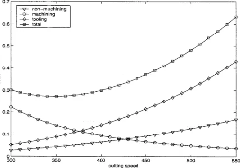
An exact solution of the geometric programming formulation given in Step 1.1 can be found in a polynomial time as discussed in Akturk and Avci (1996) . The proposed formulation can be very helpful in de® ning the in¯ uence of the machining conditions on the total manufacturing cost as depicted in ® gure 1. If we increase
either vpij or fpij, or both, then we can reduce the machining time, but this will
increase the tool usage, and equivalently non-machining and tooling costs. On the other hand, a heavy feed rate is conducive to formation of a built-up edge and a rough surface ® nish. Whereas high cutting speed improves the surface ® nish since it decreases the built-up edge formation on the face of a cutting tool. This paper makes a distinction between the machining time and the processing time. Machining time is de® ned as the time required to complete a metal cutting operation, which is the actual value-added operation, without considering the non-value adding compon-ents of non-machining times, such as tool replacing, tool changing, etc. Obviously, the actual processing time in practice will include both the machining and non-machining times. Therefore, the total processing time is the sum of non-machining and non-machining time components. However, it is not possible to calculate the exact non-machining time without knowing the current status of the tool magazines. Therefore, we initially approximate the expected non-machining time in terms of
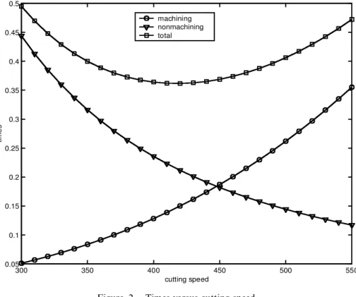
the usage rate and tool replacing time, and the processing time, t ˆ tmpij‡ Upijtrj. The
machining time is a strictly decreasing function of cutting speed, whereas the non-machining time is a strictly increasing function because of an increased usage rate a larger number of tool changes might be required (® gure 2). Therefore, there exists a trade-oŒbetween the total manufacturing cost and the total processing time. In order to decrease the total processing time, we have to incur an additional manu-facturing cost due to an increase in the non-machining and tooling costs. Furthermore, both the total manufacturing cost and total processing time are
Figure 1. Costs versus cutting speed.
convex in terms of the cutting speed. In order to prove convexity, it will be su cient
to show that tmpij and Upij are convex in terms of vpij since any positive linear
combination of these functions will be also convex. If we take the second derivatives of both functions: ¯2tmpij ¯ v2 pij ˆ2ºDpiLpi 12v3 pij fpij > 0 and ¯ 2U pij ¯ v2 pij ˆºDpiLpid ®j pi…¬j 1†¬j 12Cjv 1 ¬j pij f 1 j pij > 0:
That means tmpij is a strictly decreasing and Upij is a strictly increasing convex
func-tions of vpij. The interval in which the processing times can vary is de® ned by the set
of constraints. Akturk and Avci also prove that at least one of the surface roughness and machine power constraints is binding at optimality for SMOP. Thus, the machining conditions should always be set to a point on the boundary of the feasible region (® gure 3). The portion of the boundary, where the processing times can be controlled, is called the e cient frontier and is determined according to the opera-tional and tooling parameters. We will explain the derivation of the e cient frontier for a single operation on a numerical example in Section 5.3.
In order to ® nd out the e cient frontier, we should ® rst ® nd four critical …v; f †
pairs. The ® rst pair …v1; f1† gives the machining conditions that minimize the
manu-facturing cost. In order to ® nd the machining conditions that minimize the
pro-cessing time, there are three possibilities, namely …v2; f2†, …v3; f3† and …v4; f4†. The
second pair …v2; f2† is the intersection point at which both surface roughness and
machine power constraints are tight.
Integrated scheduling and tool management in FMS
300 350 400 450 500 550 0.05 0.1 0.15 0.2 0.25 0.3 0.35 0.4 0.45 0.5 cutting speed tim es machining nonmachining total
Figure 2. Times versus cutting speed.
v2ˆ …Cs=SF†…c†=…hb gc†…Cm=HP†… h†=…hb gc†d…Ic he†=…hb gc†
and
f2ˆ …Cs=SF†…b†=…gc hb†…Cm=HP†… g†=…gc hb†d…Ib ge†=…gc hb†:
The third pair …v3; f3† is the one that minimizes the total processing time on the
surface roughness boundary. In order to ® nd this pair, ® rst we write the feed rate in
terms of cutting speed using the surface roughness constraint as
f ˆ …SF=Cs†1=hd I=hv g=h, then substitute this in the processing time expression
tˆºDL12 ¢ …Cs=SF†1=hdI=h v…g h†=h‡ …Cs=SF† =h¢ d…®h I†=h¢ trj Cj¢ v …h…¬ 1† g… 1††=h ³ ´ : We take the derivative of t with respect to v and solve the obtained expression for v
to get v3. Finally, we substitute v3in the equation for f to get f3. However, the third
pair of …v3; f3† will be on the e cient frontier if v3< v2since the surface roughness
constraint is tight for velocities up to v2.
The last pair …v4; f4† is the one that minimizes the total processing time on the
machine power boundary, hence we de® ne the feed rate in terms of cutting speed using the machine power constraint, substitute this in the processing time expression,
and take the following derivative to ® nd v4:
dt dvˆ ºDL 12 …Cm=HPmax† 1=cde=cv…b=c† 2 £ bc c‡ …Cm=HPmax† =cd…®c e†=c trj Cj b… 1† ‡ c…¬ 1† c v …c¬ b †=c ³ ´ :
If both …b=c 1† and …c…¬ 1† b… 1††=c are non-negative, not
simul-taneously being zero, processing time will be a strictly increasing function of the
velocity. Thus, the machine power constraint will not be active. If both …b=c 1† and
…c…¬ 1† b… 1††=c are non-positive, not simultaneously being zero, processing
Figure 3. Fesible region.
time will be a strictly decreasing function of velocity. However, this case is
impos-sible, since ¬ > > 1, hence …¬ 1†=… 1† > 1. If one of …b=c 1† and
…c…¬ 1† b… 1††=c is positive and the other is negative, there is a pair …v4; f4†
where it gives the minimum total processing time. v4 can be solved by setting the
derivative to zero and the corresponding f4 can be obtained. However, the fourth
pair of …v4; f4† will be on the e cient frontier if v4> v2 since the machine power
constraint is tight for velocities over v2.
Hence, we can explicitly de® ne the e cient frontier as follows:
If …v2µ v3†^ either …b=c < 1 ^ v2> v4† or …b=c > 1 ^ …¬ 1†=… 1† > b=c†
or …b=c > 1 ^ …¬ 1†=… 1† < b=c ^ v2> v4†
then the efficient frontier is from …v1; f1† to …v2; f2†;
else either …b=c < 1 ^ v2µ v4† or …b=c > 1 ^ …¬ 1†=… 1† < b=c ^ v2µ v4†
then the efficient frontier is from …v1; f1† to …v4; f4†
If …v2> v3†^ either …b=c < 1 ^ v2> v4† or …b=c > 1 ^ …¬ 1†=… 1† > b=c†
or …b=c > 1 ^ …¬ 1†=… 1† < b=c ^ v2> v4†
then the efficient frontier is from …v1; f1† to …v3; f3†;
else either …b=c < 1 ^ v2µ v4† or …b=c > 1 ^ …¬ 1†=… 1† < b=c ^ v2µ v4†
then the efficient frontier is from …v1; f1† to …v3; f3† and from …v2; f2† to …v4; f4†:
For the last case, the e cient frontier is discontinuous, therefore some of the points in the second part might have a higher value in terms of the total processing time than the ones in the ® rst part. Thus, in order to ® nd the relevant range of the
second part, the value of the processing time at …v3; f3† can be calculated and the
expression for t for the second part can be solved to ® nd a new v, called v5. If v5< v2,
then the second part starts from …v2; f2†, otherwise f5 corresponding to v5is found
and the second part starts from …v5; f5†.
3.2. Initial schedule
In order to ® nd an initial schedule that will minimize total production cost, we propose two ranking indices. The ® rst one is used for choosing the machine that each part type can be loaded on, and the other one is used for choosing the part type that will be processed. In the proposed scheduling algorithm, we are scheduling all parts
of a particular part type in a given batch size, Qp, i.e. lot splitting is not allowed.
Since the non-machining times are state-dependent, we schedule one part type at a time and recalculate the non-machining times of the unscheduled part types after each assignment to consider the actual tool sharing possibilities. It is important to note that the shop orders of diŒerent part types will correspond to diŒerent customer requirements in terms of the required batch sizes, due dates, etc. Furthermore, ® rms have a variety of customers, some of which are more important than others. The
importance of a customer order for a certain part type, wp, can depend on a variety
of factors, e.g. the ® rm’s length of relationship with the customer, how frequently they provide business to the ® rm, and the potential of a customer to provide orders in the future. Therefore, it is important for manufacturing to re¯ ect these priorities in
Integrated scheduling and tool management in FMS
their scheduling decisions. In addition, in the presence of job tardiness penalties, it may not be enough to measure the shop ¯ oor performance by employing unweighted performance measures alone which treat each job in the shop as equally important.
The ® rst index is the machine preference ranking index, MIpm, for each part type,
p, machine, m, pair given by the following equation:
MIpmˆ wp
…tmpm ‡ tspm†
…DDp tcm …tmpm‡ tspm††: …27†
This index is a combination of weighted shortest processing time and the minimum slack time rules. As indicated above, the total processing time of a part type consists of machining and non-machining time components. The proposed index gives a higher priority to the machine which is faster and requires less total non-machining time. The machine with the highest index becomes the preferred machine of that part
type. The machining time of the part type, tmpm, is the same for all machines, which is
determined according to the machining conditions selected at the ® rst level.
However, the non-machining time, tspm, required for a part type will be diŒerent
on each machine, since the tool replacing time depends on the number of tool replacements related to the current status of the tool magazines of the machines.
The proposed ranking index is a dynamic rule because it is a function of the time tcm
at which the machine m became free, as well as the wp, DDp, tmpm and the current
status of the tool magazine to calculate tspm.
When we schedule a part type on a certain machine, the current status of the tool magazine of that machine usually changes, since the new part type either might require new additional cutting tools to be loaded or the existing tools on the tool magazine may not have enough remaining tool life. Therefore, this machine is called
`an altered machine’, because both tcm(the completion time of the last scheduled part)
and tspm of the unscheduled part types on this machine will be recalculated according
to the new status of the tool magazine. For the remaining m 1 machines, the
current machine ranking indexes will remain the same.
In the calculation of the non-machining time for a part type p on machine m, tspm,
we ® rst try to ® nd how many parts of the batch can be processed by the tools currently present on the tool magazine. In order to ® nd the actual tool sharing possibilities between the parts, we keep track of the exact remaining tool lives of each tool on the magazine. When a single copy of a tool is used for the whole batch,
the remaining tool life, …rlifej†, can be found as rlifej ˆ 1 …QpUpij†. However, if
multiple copies of a tool are used, we have to ® nd how many parts are processed by the last tool in order to ® nd the remaining tool life. First, we ® nd the number of
parts that can be processed by a single tool given by rpij. Then we sum up the number
of parts that are processed up to the last tool and subtract this from the batch size to ® nd the number of parts for the last tool, which is multiplied by the usage rate to ® nd the remaining life of the tool currently loaded on the magazine as follows:
rlifej ˆ 1 …Qp …npij 1†rpij†Upij. If the whole batch cannot be processed by the
tools present on the magazine and the magazine is full then an additional non-machining time will be incurred since one of the currently loaded tools must be unloaded to open up a new slot. The tool that will be unloaded is chosen as the one either that has zero remaining life or that has the shortest remaining life and is not required for the part in consideration.
The second index is the part ranking index, PIpm, given by the following equa-tion: PIpmˆ wp …tmpm‡ tspm† exp ( max fDDp tcm …tmpm‡ tspm†; 0g k¤ ·ppm ) : …3†
This index is calculated for each part type on its preferred machine which is deter-mined according to the ® rst index. The proposed index gives a higher priority to the part type which can be processed faster and has a less slack time. The main aim of this index is to reduce the amount of weighted tardiness.
In the second level, we ® rst determine the preferred machine of each part type using the ® rst index, and then select the part type which will be loaded using the second index. Once a part type is chosen to be loaded, the current status of the tool magazine is updated according to the necessary tool loadings and unloadings. The remaining tool lives are also recalculated by subtracting the usage amount of the loaded part from the initial tool lives. After we ® nish loading a part type, we recal-culate the non-machining times required for the unscheduled part types only on the
altered machine, and calculate the indexes MIpm and PIpm to choose the next part
type to be loaded. We repeat this procedure until all part types are scheduled. We can illustrate this level step by step as follows:
Step 2.1. Since initially all the tool magazines are empty, there is no diŒerence
between the machines. For each part type calculate the index PIpm and
select the part type with the highest PIpm to load on the ® rst machine.
Step 2.2. After loading of a part type is completed, calculate the remaining lives of
the tools currently loaded on the magazine and the average processing
time, ·ppm, of the unscheduled part types for each unaltered machine. On
the other hand, calculate the non-machining time requirement of each unscheduled part type only on the altered machine.
Step 2.3. Initially calculate the index MIpm for all machines in order to choose the
preferred machine for each unscheduled part type. However, after the ® rst
iteration, the index MIpm should be calculated for only the altered
machine, since it will remain the same for the unaltered machines.
Step 2.4. After calculating the index PIpm on the preferred machine for each part type, load the part type with the maximum index to its preferred machine.
Step 2.5. If any tool with remaining life greater than zero but smaller than the
minimum fUpijg is to be removed from the magazine, we check all the
operations using this tool and increase the cutting speed of the most ben-e® cial operation as much as possible to decrease the total production cost. Go to Step 2.2 until all part types are scheduled.
In sum, the non-machining time is a state-dependent variable, and it depends on the current arrangement of the tool magazine, i.e. which tools are loaded and their respective remaining tool lives. Therefore, we have to keep track of the state of the tool magazine after scheduling a certain part type that means we remove some cutting tools and add new ones, if necessary, and update the remaining tool lives for the tools that will be used to manufacture the given batch size. One of the primary objectives in the proposed algorithm is to minimize the total weighted tardiness. The reason we schedule one part type at a time is to calculate the slack values of each part type accurately. The slack value for each part type,
Integrated scheduling and tool management in FMS
DDp tcm …tmpm‡ tspm†, is not constant and changes over time, since both t
c m and
tspm are not constant, and depend on the current tool magazine arrangement of
machine m and the set of part types that are already scheduled on machine m.
3.3. Final schedule
At the end of the ® rst level, we obtain the tool allocations with their governing machining conditions. In this level, we not only determine the primary tool for any operation, but also ® nd the best alternative tool for the same operation. At the third level, we allow that the processing times can be controlled via either the cutting speed or the feed rate. We choose the cutting speed as our controllable variable and determine the feed rate accordingly. Besides reducing the processing time by using the primary tool, we also consider alternative tool usage and batch splitting at this level if there is not su cient slack amount of the primary tool. The third level can be considered as a left shift procedure, where we retain the same sequence found in the second level, but the starting times are shifted to the left in a Gantt chart representa-tion by decreasing the processing times as much as possible to decrease the total production cost.
In order to ® nd the e cient frontier, we classify each operation according to their tooling and operational parameters. We use piecewise linearization to approximate the non-linear e cient frontier into pieces of equal cutting speed range. If the last remaining piece has a shorter cutting speed range than the ® xed step size, we will add it to the previous piece, otherwise we will consider it as a single piece. After doing the piecewise linearization, we propose a ranking index for each piece to choose the operation that will be crashed. This index shows us the opportunity cost-related to
tardiness cost. The index of piece s of operation i of part p, TIpis, is de® ned as:
TIpisˆ ¢TC ¢t ³ ´ X k wk: ,
¢TC shows us the increase in the total manufacturing cost consisting of the machining, non-machining and tooling costs, when we crash the processing times.
Since …v1; f1† is the optimum solution for the total manufacturing cost, any …v; f †
pair other than …v1; f1† will give a higher total manufacturing cost. ¢t represents the
total gain in the processing time as a result of the crashing. The numerator of the proposed index shows the increase in the total manufacturing cost for the time gain in the processing time, whereas the denominator shows the total gain in terms of tardiness cost, when a unit reduction in the total processing time of that operation is achieved. After calculating the index for each piece of every operation, we choose the
most bene® cial operation, that is the one with the smallest TIpis, so that a unit gain in
tardiness cost can be achieved with less cost. In sum, we start with the initial schedule and then look for the operation when it is crashed that results in the `biggest bang for the buck’ with respect to production cost improvement.
After choosing the most bene® cial operation, if we have enough slack of the required tool to speed up the operation, we crash its processing time and ® nd the new starting times of each part type on this machine. Otherwise, we consider the alternative tools to perform the same operation. If we have any gain in
pro-cessing time when we use the alternative tool, i.e. tini> talt, then we calculate an
alternative tooling index of operation i of part p, ATIpi, as follows:
ATIpiˆ…TCalt TCini† …tini talt† X k wk; ,
where TCalt and TCini are the total manufacturing cost of operation i using the
alternative and primary tools, respectively. Similarly, talt and tini show the total
processing time of the alternative and primary tools, respectively. The numerator of the index again gives the additional cost incurred for unit time gain in the pro-cessing time when an alternative tool is used, whereas the denominator gives the total gain in tardiness cost for a unit reduction in the processing time. If this index < 1, then we allow batch-splittin g and calculate the amount of parts that can be processed by the primary tool and process the remaining parts with the alternative tool. The steps of the third level can be given as follows:
Step 3.1. For every part-operation pair, determine the e cient frontier where the
processing time can be controlled as discussed in Section 3.1
Step 3.2. Using piecewise linearization, calculate the index TIpis for each piece and
sort the indices in increasing order. Select the smallest TIpis value.
Step 3.3. If there is enough slack of the required tool to meet the increased usage due
to higher velocity, recalculate the total machining and setup time for the part type of this triple …p; i; s† and left shift the parts on the machine where the selected part type is scheduled.
Step 3.4. If there is not enough amount of primary tool and alternative tool usage is
bene® cial, i.e. ATIpi< 1, then repeat Step 3.3 for an alternative tool.
Step 3.5. Recalculate the index values for the remaining operations and repeat the
above procedure until there is no more bene® cial operation to be crashed,
i.e. both TIpis and ATIpi> 1 for every operation i of part type p.
4. Experimental design
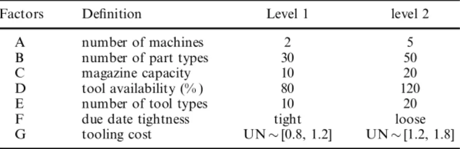
In this section we test the e ciency of the proposed algorithm by comparing with some of the existing algorithms in the literature. All of the algorithms are coded in the C language and compiled with Gnu C compiler. The IP formulation in the ® rst level of the proposed algorithm is solved by using callable library routines of CPLEX MIP solver on a Sparc station 10 under SunOS 5.4. There are seven experimental factors that can aŒect the e ciency of our algorithm, which are listed in table 1. The
experimental design is a 27 full-factorial design as there are seven factors with two
levels each. The number of replications of each combination is taken as ® ve produ-cing 640 diŒerent randomly generated runs.
Integrated scheduling and tool management in FMS
Factors De® nition Level 1 level 2
A number of machines 2 5
B number of part types 30 50
C magazine capacity 10 20
D tool availability (% ) 80 120
E number of tool types 10 20
F due date tightness tight loose
G tooling cost UN ¹ [0.8, 1.2] UN ¹ [1.2, 1.8] Table 1. Experimental factors.
The number of machines and part types determine the size, product mix and load of the system. As the number of machines or part types increases, the scheduling decision becomes more important. The magazine capacity, which is identical for each machine, determines the number of tools that can be loaded simultaneously to the machine. It aŒects the actual setup time required for the parts. The fourth factor speci® es the tightness of the tool availability constraint. The number of available tools on hand is taken as 80 and 120% of the required amount of tools for each tool type at low and high levels, respectively. The ® fth factor is the number of tool types. As the number of tool types increases, the operation-tool assignment alternatives increase. The sixth factor is used to determine the due dates of the part types. In the tight case, due dates are randomly generated in the ® rst half of the estimated make-span, whereas in the loose case, due dates are distributed in a wider range. The estimated makespan, MS, is calculated by dividing the sum of processing times to the number of machines. In the tight case, the due dates are chosen from the interval UN ¹ [0.1 ¢ MS, 0.5 ¢ MS], whereas, in the loose case, due dates are chosen from the interval UN ¹ [0.2 ¢ MS, 0.8 ¢ MS], where UN stands for the uniform distribution. Finally, the seventh factor is the tooling cost, which is likely to aŒect operation-tool assignments and the crashing decisions at the ® nal level.
Other variables are treated as ® xed parameters and generated as follows. The
operating cost, Co, is equal to 0.5/min, and HP ˆ 5 h.p. The operation related
par-ameters, Dpi and Lpi, are selected randomly from the interval UN ¹ [1.5, 2.5] and
UN ¹ [5, 7], respectively. Batch sizes are selected from a discrete distribution with
probability mass function of fQ…q† ˆ f0:3 when Q ˆ 10; 0:4 when Q ˆ 15, and 0.3
when Q ˆ 20g. The number of operations per part is chosen from an integer interval UN ¹ [3, 5], and the last operation of each part is taken to be a ® nishing operation
whereas the remaining operations to be roughing operations. SFpiand dpiare related
with the type of operations. For roughing operations, SFpiˆ UN ¹ ‰300; 500Š and
dpiˆ UN ¹ ‰0:2; 0:3Š, and for the ® nishing operation, SFpiˆ UN ¹ ‰30; 70Š and
dpiˆ UN ¹ ‰0:025; 0:075Š. The weight of each part type is chosen from the integer
interval UN ¹ [1, 3].
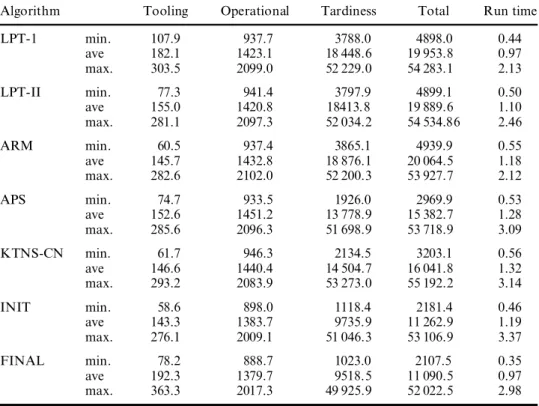
Five performance measures are used for comparison purposes, which are tooling, operational, tardiness and total production costs, and run time. The tooling cost is the total cost of tool usage in the system. The operational cost is the sum of machin-ing and non-machinmachin-ing time costs, i.e. the total cost of operatmachin-ing the CNC machines. The tardiness cost is the total weighted cost of the part types that are tardy. The total production cost is the sum of these three cost terms. Finally, the run time is the computation time in seconds.
The experimental design is also applied to ® ve existing algorithms in the litera-ture, which are LPT-I, LPT-II, ARM, APS, and KTNS-CN. The ® rst four are developed by Kim and Yano (1993) and the last one is proposed by Askin and Standridge (1993). In the LPT-I and LPT-II algorithms, the part type with the longest processing time is assigned to the machine which has the minimum load after the part type is assigned to it. The main diŒerence between these two algorithms is that the ® rst one ignores tool sharing possibility between the parts and therefore uses the constant setup time value calculated at the beginning. However, the second algorithm considers actual tool sharing possibilities and recalculates the setup time required for each unscheduled part type after a part type is loaded to a machine. ARM loads the unscheduled part type with the largest T/S to the machine with the largest T/S. The T/S ratio for a machine is the ratio of the remaining processing time
capacity of the machine to the remaining tool magazine capacity. The T/S ratio for a part type is the ratio of the processing time of the part type to the number of tool slots required for the part type. Each part type might have a diŒerent T/S ratio for each machine due to tool commonality. The basic idea of the ARM selection cri-terion is that larger items are packed in larger bins to achieve a better loading. APS loads the part type that requires the largest number of tool slots on the most pre-ferred machine to that machine. The most prepre-ferred machine for a part type is the one on which minimum setup time is required. Tang and Denardo (1988) prove that the common sense rule keep tool needed soon (KTNS) is optimal for changing the tool magazine when there is a deterministic change time and all changes are due to part mix, ignoring tool changes due to tool wear. KTNS-CN algorithm by Askin and Standridge removes only as many tools as necessary to make way for the next part type. The tools removed are those that will not be needed again until the longest time in the future and loads the part type that requires the minimum setup time on its most preferred machine, in other words, the closest neighbour to the current status. All of these algorithms use only 0± 1 type variables when assigning tools to operations, although there may be cases where a single operation requires duplicate tools. They do not consider tool lives and assume that any tool can perform two to four part types. Their approach can be considered as a complete sharing. However, this might be an unrealistic assumption, since the tool life is dependent on the machining conditions and it may not be possible for each tool to be shared by the parts due to their usage amounts. Processing times are assumed to be ® xed, and chosen from some probabilistic distribution. They do not consider the fact that processing times can be controllable via either the cutting speed or the feed rate. Finally, they do not consider alternative tool assignments for the operations. In order to make these algorithms comparable with our proposed algorithm, we modify them to consider duplicate tooling and actual tool lives.
The overall results of the algorithms are summarized in table 2. The table shows the minimum, average and the maximum values for the performance measures for all of the algorithms. INIT corresponds to the initial schedule of the proposed algor-ithm found after the second level, whereas the ® nal schedule is denoted by FINAL. In sum, the average performance of the proposed algorithm is signi® cantly better than the algorithms used in the literature in terms of the total production cost, although it requires a relatively higher computation time.
For the tooling cost, INIT gives the minimum average tooling cost, whereas FINAL gives the maximum average tooling cost. The reason why it gives the mini-mum at the initial schedule is that all tool sharing possibilities are evaluated. However, at the ® nal schedule, in order to decrease the total cost, we increase tool usage which in turn results in higher tooling cost. LPT-I gives the highest tooling cost among the other algorithms, since it does not consider tool sharing possibility among parts. When we interpret the operational cost values, we see that our pro-posed algorithm results in the minimum average operational cost. The propro-posed algorithm has the minimum average tardiness cost as expected which is far below the tardiness costs of other algorithms, since they do not consider the scheduling problem while solving the tool management problem. For the total cost, the best average performance is achieved again by the proposed algorithm. Finally, LPT-I is the fastest algorithm in terms of run times as expected since it only calculates the setup time at the beginning and uses the same value throughout the algorithm.
Integrated scheduling and tool management in FMS
However, other algorithms recalculate the setup times at each iteration. The run times of ® nal schedule show the additional time required over the initial schedule.
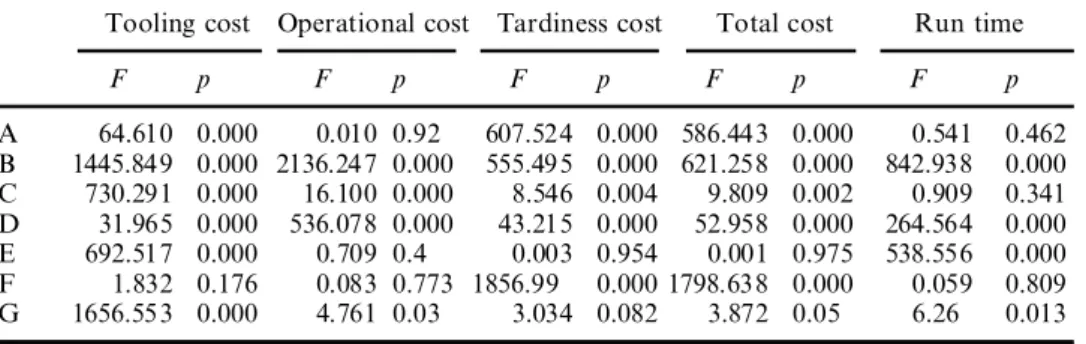
We also applied a two-way analysis of variance (ANOVA) test on the perform-ance measures. The signi® cperform-ance levels …p† and F for each of them over seven factors are given in table 3. For the tooling cost, all the factors except the due date tightness are signi® cant with p µ 0:000. Among them, the factor B speci® es the total tool requirement, the factor G determines unit tooling costs, whereas factors A and C restrict the tool sharing possibilities, hence aŒect the tooling cost incurred. Factors D and E limit the number of tools on hand, hence the allocation decisions. For the operational cost, only three factors are signi® cant with p µ 0:000. These are number of part types, tool magazine capacity and tool availability. The factor B determines the load on the system, therefore the cost of producing the parts. The factor C limits the tool sharing possibility, and hence aŒects the non-machining time. The factor D restricts the number of tools on hand. Each operation cannot always be assigned to its best tool alternative due to the tool availability constraints. Hence, this will result in increased machining times and consecutively increased total operational cost. For the tardiness cost, the factors A, B, D and F are signi® cant with p µ 0:000. The estimated makespan is a function of factors A, B and D, whereas the factor F directly determines the due date range of the part types.
We can summarize our ® ndings as follows. The FMS design parameters of number of machines, part types and alternative cutting tool types, tool availabilities and tool magazine capacities have a signi® cant impact on the operational decisions of part scheduling and tool management. As the load of the system increases, the
Algorithm Tooling Operational Tardiness Total Run time
LPT-1 min. 107.9 937.7 3788.0 4898.0 0.44 ave 182.1 1423.1 18 448.6 19 953.8 0.97 max. 303.5 2099.0 52 229.0 54 283.1 2.13 LPT-II min. 77.3 941.4 3797.9 4899.1 0.50 ave 155.0 1420.8 18413.8 19 889.6 1.10 max. 281.1 2097.3 52 034.2 54 534.86 2.46 ARM min. 60.5 937.4 3865.1 4939.9 0.55 ave 145.7 1432.8 18 876.1 20 064.5 1.18 max. 282.6 2102.0 52 200.3 53 927.7 2.12 APS min. 74.7 933.5 1926.0 2969.9 0.53 ave 152.6 1451.2 13 778.9 15 382.7 1.28 max. 285.6 2096.3 51 698.9 53 718.9 3.09 KTNS-CN min. 61.7 946.3 2134.5 3203.1 0.56 ave 146.6 1440.4 14 504.7 16 041.8 1.32 max. 293.2 2083.9 53 273.0 55 192.2 3.14 INIT min. 58.6 898.0 1118.4 2181.4 0.46 ave 143.3 1383.7 9735.9 11 262.9 1.19 max. 276.1 2009.1 51 046.3 53 106.9 3.37 FINAL min. 78.2 888.7 1023.0 2107.5 0.35 ave 192.3 1379.7 9518.5 11 090.5 0.97 max. 363.3 2017.3 49 925.9 52 022.5 2.98
Table 2. Comparison of the performance measures of algorithms.
scheduling and tool management interaction becomes even more important. For example, if the tool magazine capacity decreases then the tool replacements are done more frequently, hence the non-machining times increase. As the number of tool types and tool availability are at their high values, the chance to ® nd better operation-tool assignments increases and this will bring solution ¯ exibility to the system, which in turn results in lower total production cost. Obviously, there is an opportunity cost since higher tool availability will increase the tool inventory cost, whereas larger tool magazine capacity will require a higher initial investment cost. Tool costs are not only the main determinants of the total tooling cost, but also aŒect the crashing decisions available for the ® nal schedule. Finally, tool sharing is bene® cial both in terms of tooling cost and operational cost via the non-machining cost. LPT-I algorithm, which ignores the tool sharing, always gives the maximum value for the cost measures.
5. Numerical example
This section illustrates the proposed algorithm on a numerical example to point out the important steps, by focusing on each level in the following subsections. Our example problem consists of 10 part types, two machines and 10 tool types. The part
related data are summarized in table 4 and the tool related data are (tool number, trj,
tlj, tcj, ttj, trtj, Ctj, Nj)5 (1, 0.87, 1.24, 0.40, 0.13, 0.06, 1.087, 4), (2, 0.75, 1.37, 0.48,
0.14, 0.07, 1.034, 1), (3, 0.82, 1.49, 0.38, 0.10, 0.09, 1.054, 1), (4, 0.72, 1.15, 0.31, 0.15, 0.14, 1.003, 22), (5, 0.93, 1.19, 0.32, 0.16, 0.12, 1.050, 4), (6, 0.92, 1.24, 0.32, 0.18, 0.10, 1.087, 1), (7, 0.75, 1.32, 0.33, 0.18, 0.10, 0.970, 5), (8, 0.94, 1.27, 0.42, 0.15, 0.11, 1.134, 2), (9, 0.84, 1.49, 0.38, 0.12, 0.09, 0.978, 2), and (10, 0.86, 1.31, 0.48, 0.20, 0.08, 0.829, 8). Each cutting tool type might have diŒerent non-machining time compon-ents of tool replacing, changing, loading, etc., depending on whether or not the tool
Integrated scheduling and tool management in FMS
Tooling cost Operational cost Tardiness cost Total cost Run time
F p F p F p F p F p A 64.610 0.000 0.010 0.92 607.524 0.000 586.443 0.000 0.541 0.462 B 1445.849 0.000 2136.247 0.000 555.495 0.000 621.258 0.000 842.938 0.000 C 730.291 0.000 16.100 0.000 8.546 0.004 9.809 0.002 0.909 0.341 D 31.965 0.000 536.078 0.000 43.215 0.000 52.958 0.000 264.564 0.000 E 692.517 0.000 0.709 0.4 0.003 0.954 0.001 0.975 538.556 0.000 F 1.832 0.176 0.083 0.773 1856.99 0.000 1798.638 0.000 0.059 0.809 G 1656.553 0.000 4.761 0.03 3.034 0.082 3.872 0.05 6.26 0.013
Table 3. F and signi® cance levels (p) for ANOVA results.
Part type number 1 2 3 4 5 6 7 8 9 10
No. of operations 5 5 3 5 3 4 5 3 3 4
Weight 2 2 3 1 3 3 3 1 2 1
Due date 41 170 65 111 177 181 67 92 40 49
Batch size 15 15 15 15 10 15 10 15 20 15
Table 4. Part type-related information.
uses some special accessory. In our numerical example, the tool replacing time for
tool type 1, tr1 ˆ 0:87, whereas it is 0.75 for tool type 2, and so forth.
5.1. Tool allocation
As the ® rst step of this level, we solve SMOP to determine the optimum machin-ing conditions for every possible part type, operation and tool triple. We calculate the cost measure given in equation 1 for each alternative, and ® nd the …j; k† pair giving the minimum cost value for each …p; i† pair. If we consider the ® rst operation of the ® rst part type, i.e. (1,1), there are six alternative tool types that can perform
this operation and tool 7 gives the minimum cost measure since (tool number, tmpij,
TCpij)5 (1, 0.228, 2.033), (2, 0.315, 3.206), (3, 0.262, 3.008), (5, 0.134, 1.553), (7,
0.141, 1.4), and (8, 0.16, 1.53). We then compute the total requirement for each tool
type j to check tool feasibility. If Rjµ Nj for every j, then the lower bound solution
found above is optimum. Otherwise, an IP formulation given in Step 1.4 is solved to ® nd the best allocation for each operation that satis® es tool availability constraints. In our example, we assume that there is an 80% tool availability and there is no precedence relation among the operations of a part. Therefore, we have to solve an IP formulation to ® nd the optimum tool allocations. These best allocations for part type 1 can be summarized as (operation number, tool number, usage rate) triples as (1, 7, 0.134), (2, 4, 0.066), (3, 7, 0.066), (4, 4, 0.034), and (5, 4, 0.059).
Before the scheduling decision, we ® nd out tool sharing possibilities among the operations of the same part, which will result in a direct reduction in the total non-machining time required for that part. If we consider part type 1, we can gather operations using the same tool as long as their total usage rate does not exceed 1, which means that the same tool can perform both of the operations. For example,
the ® rst and third operations use tool type 7 and their total usage (0.134 1
0.066 ˆ 0.2) < 1. Therefore, we gather these two operations into a single operation, whose processing time is the sum of the processing times of the individual operations
(0.141 1 0.24 ˆ 0.381). Consequently, we reduce the non-machining time required
for each part by tc7‡ tt7 trt7ˆ 0:33 ‡ 0:18 0:10 ˆ 0:41 minute. Similarly, the
second, fourth and ® fth operations of this part can also be gathered since their total tool usage is 0.159. After gathering the possible operations, we calculate total machining and total expected set up time required for each part type to be
used in the scheduling level as follows: (part no., tm, ts)5 (1, 48.9, 4.76), (2, 104.6,
7.88), (3, 51.3, 6.31), (4, 58.2, 5.82), (5, 36.8, 3.57), (6, 73.2, 5.08), (7, 65.8, 7.48), (8, 64.1, 4.72), (9, 94.4, 5.65) and (10, 66.3, 5.19).
5.2. Initial schedule
As discussed above, we ® nd an initial schedule by utilizing two ranking indices,
MIpmand PIpm. Since all the tool magazines are empty at the initial state, there is no
diŒerence between the machines. So we just calculate the index PIpm for each part
type and load the one with the highest index to the ® rst machine. The initial PIpmare
calculated as follows: (part, PI)5 (1, 0.0373), (2, 0.0119), (3, 0.0495), (4, 0.0113), (5,
0.0259), (6, 0.0188), (7, 0.0409), (8, 0.0124), (9, 0.02) and (10, 0.014). Since part type 3 has the highest index value, it is loaded to the ® rst machine. The operations of part type 3 with their allocated tools and associated usage rates are (1, 4, 0.065) and (2, 10, 0.267). Initially, part type 3 had three operations but after the tool sharing the last two operations were aggregated into a single operation. We calculate the remain-ing tool lives of the tools currently on the magazine, which are tool type 4 and 10. A
single copy of tool 4 is used for the whole batch, therefore the remaining life is equal
to rlife4ˆ 1 …15 ¢ 0:065† ˆ 0:025. However, multiple copies of tool 10 are used
because Qp¢ Upij > 1. In order to ® nd the remaining life of the tool currently
loaded on the magazine, we have to ® nd how many parts are processed by the last
copy as discussed in Section 3.2 and rlife10 ˆ 1 …15 …4 ¢ 3†† ¢ 0:267 ˆ 0:199.
Then we update the current time of the ® rst machine, which becomes the completion time of the last loaded part type to that machine, hence
tc1ˆ 51:3 ‡ 6:31 ˆ 57:61. Next, we calculate the average processing time of
unsched-uled part types on the second machine, i.e. ·pp2ˆ 73:51. Afterwards, we calculate the
actual setup time required on the ® rst machine and MIpmfor both machines for each
unscheduled part type in order to choose the preferred machine for each part type. However, in this example after the initial loading of part type 3 to the ® rst machine, there is no diŒerence in the setup times on the machines for each part type.
Therefore, we will not calculate MIpm. All the part types will prefer the machine
at which they can start earlier to have more slack time. The second machine becomes the preferred one and part type 7 is assigned to it in the second iteration, The remaining tool lives of the tools on the second machine are calculated and the current time of the second machine is set equal to the completion time of part type 7. We repeat these steps until there is no more unscheduled part types.
Let’s explain this procedure in detail after the partial schedule of M/C 1: f3 5 -6g, and M/C 2: f7 - 1 - 9g. In the previous iteration, part type 9 is loaded to the second machine. Therefore, the setup time required on the second machine for the unscheduled part types, which are 2, 4, 8 and 10, should be recalculated due to the changes in the current status of the magazine. As an example, the calculations done for the part type 2 are shown below.
tm21 ˆ tm22ˆ Qp¢ …tm216‡ tm224‡ tm236‡ tm244‡ tm253‡ 2…tc6‡ tt6† ‡ 2…tc4‡ tt4†
‡ 2…tc3‡ tt3† ‡ trt6‡ trt4† ˆ 15 ¢ …0:765 ‡ 1:224 ‡ 0:611 ‡ 0:689 ‡ 0:567
‡ 2…0:32 ‡ 0:18† ‡ 2…0:31 ‡ 0:15† ‡ 2…0:38 ‡ 0:10† ‡ 0:10 ‡ 0:14† ˆ 104:6
ts22ˆ tl3‡ tl4‡ tl6‡ …3 ¢ tr4† ‡ tr6 ˆ 1:49 ‡ 1:15 ‡ 1:24 ‡ …3 ¢ 0:72† ‡ 0:92 ˆ 7:08:
Similarly, ts21 is calculated to be 8.20. After ® nding the total machining and
non-machining times for part type 2, we calculate the machine preference index given by equation 2.
MI21 ˆ …2=…104:6 ‡ 8:2†† ¢ …170 176:26 …104:6 ‡ 8:2†† ˆ 2:114:
MI22 is found to be ± 2.992 by the same way. Since MI21 is greater than MI22,
second machine is preferred by part type 2. Then we calculate the index PI21given by
equation (3).
PI21ˆ …2=…104:6 ‡ 8:2†† ¢ exp f max f170 176:26 …104:6 ‡ 8:2†; 0g=…2 ¤ 80:04†g
ˆ 0:0181:
The results of these calculations for all unscheduled part types are shown in table 5. Since part type 2 has the highest index value, it is loaded to the ® rst machine. The initial schedule obtained at the end of this level is presented in tables 6 and 7 for the ® rst and second machines, respectively. The cost components of the initial schedule
Integrated scheduling and tool management in FMS