Başlık: Separation axioms in Ćech closure ordered spacesYazar(lar):EROGLU, İrem; GUNER, ErdalCilt: 65 Sayı: 2 Sayfa: 001-010 DOI: 10.1501/Commua1_0000000754 Yayın Tarihi: 2016 PDF

(1)

C O M M U N I C A T I O N S

Series A1:

Mathematics and Statistics

VOLUME: 65 Number: 2 YEAR: 2016

Abstracted in

Mathematical Reviews (MathSciNet), Zentralblatt MATH (ZbMATH) , TUBITAK-Ulakbim

Faculty of Sciences, Ankara University 06100 Beşevler, Ankara-Turkey

ISSN 1303-5991

DE LA FACULTE DES SCIENCES

DE L’UNIVERSITE D’ANKARA

FACULTY OF SCIENCES

ANKARA UNIVERSITY

(2)

C O M M U N I C A T I O N S

DE LA FACULTE DES SCIENCES FACULTY OF SCIENCES DE L’UNIVERSITE D’ANKARA ANKARA UNIVERSITY

Series A1: Mathematics and Statistics

Owner Hüseyin BEREKETOĞLU Editor in Chief Nuri ÖZALP Managing Editor Erdal GÜNER Area Editors

Sait HALICIOĞLU (Group Theory) Elif DEMİRCİ (Applied Mathematics) Gülen TUNCA (Analysis-Theory of Functions) Murat OLGUN (Functional Analysis)

Yusuf YAYLI (Geometry) İshak ALTUN (Topology)

Yılmaz AKDİ (Statistics) Murat ŞAHİN(Number Theory) Burcu Ungor (Rings and Modules Theory)

Editors

M.AKHMET METU, TURKEY O. ARSLAN Ankara Uni. TURKEY A. AYTUNA Sabancı Uni. TURKEY E. BAIRAMOV Ankara Uni. TURKEY H. BEREKETOĞLU Ankara Uni. TURKEY H. BOZDOĞAN Uni. of Tennessee, USA C.Y.CHAN, Univ. of Louisiana, USA A. B. EKİN Ankara Uni. TURKEY D. GEORGIOU Uni. of Patras GREECE V. GREGORI Uni. Politècnica de València, SPAIN I. GYORI Veszprem Uni. HUNGARY A. HARMANCI Hacettepe Uni. TURKEY F.HATHOUT Uni. de Saïda, ALGERIA K. ILARSLAN Kırıkkkale Uni. TURKEY A. KABASINSKAS Kaunas U. of Tech., LITHUANIA V. KALANTAROV Koç Uni. TURKEY F. KARAKOC Ankara Uni. TURKEY A. M. KRALL The Penn. State Uni. USA H.P. KUNZI Uni. of Cape Town, SOUTH AFRICA S. KOKSAL, Florida Inst. of Tech. USA H.T. LIU, Tatung Univ. TAIWAN S. ROMAGUERA Un.Pol.de València, SPAIN C. ORHAN Ankara Uni. TURKEY C. TEZER METU TURKEY A.D. TÜRKOĞLU Gazi Uni. TURKEY S. YARDIMCI Ankara Uni. TURKEY C. YILDIZ Gazi Uni. TURKEY

This Journal is published two issues in a year by the Faculty of Sciences, University of Ankara. Articles and any other material published in this journal represent the opinions of the author(s) and should not be construed to reflect the opinions of the Editor(s) and the Publisher(s).

Correspondence Address:

COMMUNICATIONS EDITORIAL OFFICE

Ankara Üniversitesi Fen Fakültesi, 06100 Tandoğan, ANKARA – TURKEY

Tel: (90) 312-212 67 20 Fax: (90) 312-223 23 95

e-mail: commun@science.ankara.edu.tr

Print:

Ankara Üniversitesi Press İncitaş Sokak No:10 06510 Beşevler ANKARA – TURKEY

Tel: (90) 312-213 65 65 Publication Year : 2015

(3)

C O M M U N I C A T I O N S

Volume 65 Number : 2 Year :2016 Series A1: Mathematics and Statistics

I. EROGLU, E. GUNER, Separation axioms in Cech closure ordered spaces …... 1 A. TUNCER, Survival probabilities for compound binomial risk Model with discrete phase-type claims ………... 11 T. GULSEN, E. YILMAZ, Inverse nodal problem for p-Laplacian diffusion equation with polynomially dependent spectral parameter ...………. 23 T. ERMİŞ, Ö. GELİŞGEN, On an extension of the polar taxicab distance in space ….. 37 H. KADIOĞLU, On the prolongations of homogeneous vector bundles …..……… 47 H. ŞİMŞEK, M. ÖZDEMİR, On focal surfaces formed by timelike normal rectilinear congruence ………..……… 55 T. YURDAKADIM, Some Korovkin type results via power series method in modular spaces ………... 65 Y. ALTIN, 𝜆 −almost difference sequences of fuzzy numbers ……… 77 E. BAS, Inverse singular spectral problem via Hocshtadt-Lieberman method ……..…. 89 A.KARAISA, A. ARAL, Some approximation properties of Kantorovich variant of

Chlodowsky operators based on q-integer ………...……….. 97

E. DENIZ, Quantitative estimates for Jain-Kantorovich operators . .………. 121 M. YILDIRIM, K. İLARSLAN, Semi-parallel tensor product surfaces in

semi-Euclidean spaceE₂⁴ ……… 133

N. BAYRAK GÜRSES, O. BEKTAS, S. YUCE, Special Smarandache curves in

ℝ1 3 ……….………... 143

B. ZEYNEP TEMOCIN, A. S. SELCUK-KESTEL, Estimation of earthquake insurance premium rates: Turkish catastrophe insurance pool case ……… 161 E. KIZILOK KARA, S. ACIK KEMALOGLU, Portfolio optimization of dynamic copula models for dependent financial data using change point approach ………. 175 K. R. KAZMI, SHAKEEL A. ALVI, Sensitivity analysis for a parametric multi-valued implicit quasi variational-like inclusion ………... 189

(4)

C O M M U N I C A T I O N S

DE LA FACULTE DES SCIENCES FACULTY OF SCIENCES DE L’UNIVERSITE D’ANKARA ANKARA UNIVERSITY

(5)

C o m m u n . Fa c . S c i. U n iv . A n k . S é r. A 1 M a t h . S ta t . Vo lu m e 6 5 , N u m b e r 2 , P a g e s 1 –1 0 ( 2 0 1 6 )

D O I: 1 0 .1 5 0 1 / C o m m u a 1 _ 0 0 0 0 0 0 0 7 5 4 IS S N 1 3 0 3 –5 9 9 1

SEPARATION AXIOMS IN µCECH CLOSURE ORDERED SPACES

IREM EROGLU AND ERDAL GUNER

Abstract. In this paper, we generalize closure spaces by an preorder and we give some order seperation axioms in µCech closure ordered spaces.

INTRODUCTION

Topological spaces can be generalized by many ways. Leopoldo Nachbin[6] de-veloped a way to generalize topological spaces by an order. He de…ned topological ordered spaces, such that a triple (X; ; ) where is a topology and is a rela-tion of partial order on X: He investigated some properties of topological ordered spaces.

In 1968 McCartan[9] studied Ti ordered seperation axioms (i = 1; 2; 3; 4) in topological ordered spaces.

The other way to generalize topological spaces is closure operators. Eduard µ

Cech[4] de…ned µCech closure spaces or dually pretopological spaces. A.S.Mashhour and M.H.Ghanim[1] investigated properties of µCech closure spaces.

The aim of this paper is to de…ne µCech closure ordered spaces and investigate some ordered seperation axioms in this spaces. For topological spaces we refer the reader to R. Engelking[8]. For closure spaces we refer to [3],[7].

1. PRELIMINARIES

Now, we will give some basic de…nitions about closure spaces and orders. De…nition 1. Let X be a set. An order (partial order) on X is a binary relation

on X such that, for all x; y; z 2 X

i) x x

ii) x y and y x imply x = y

iii) x y and y z imply x z

These conditions are referred to, respectively as re‡exivity, antisymetry and tran-sivity. A set X equipped with an order relation is said to be an ordered set (or

Received by the editors: February 15, 2016, Accepted: April 14, 2016. 2010 Mathematics Subject Classi…cation. 54A05,54B05,54D10.

Key words and phrases. Closure ordered space, Ti orderedseparation axiom, µCech closure

space.

c 2 0 1 6 A n ka ra U n ive rsity C o m m u n ic a tio n s d e la Fa c u lté d e s S c ie n c e s d e l’U n ive rs ité d ’A n ka ra . S é rie s A 1 . M a th e m a t ic s a n d S t a tis t ic s .

(6)

2 IR EM ERO G LU A N D ER DA L G U N ER

partially ordered set).A relation on a set X which is re‡exive and transitive but not necessarily antisymmetric is called a quasi-order or preorder [2].

De…nition 2. Let X and Y be ordered sets. A map ' from X to Y is said to be an order-embedding if and only if the following be satis…ed x y in X i¤ '(x) '(y) in Y .

De…nition 3. Let X designate a preordered set. A subset A X is said to be decreasing if a _{b and b 2 A imply a 2 A: The smallest decreasing set containing} A will be shown by d(A): A subset A X is said to be increasing if a b and a 2 A imply b 2 A and the smallest increasing set containing A will be shown by i(A) [4]:

De…nition 4. Let us consider a topological space (X; ) equipped with a preorder . The triple (X; ; ) is called topological ordered space [5].

De…nition 5. If X is a set and u is a single-valued relation on P (X) ranging in P (X), then we shall say that u is a closure operation for X provided that the following conditions are satis…ed,

c1) u(;) = ;

c2) A u(A) for each A X

c3) u(A [ B) = u(A) [ u(B) for each A X and B X:

A structure (X; u) where X is a set and u is a closure operation for P , will be called a closure space ([1],[3]).

De…nition 6. Let (X; u) be a closure space. There is associated the interior oper-ation intu usually denoted by int, such that for each A X,

intuA = X u(X A)

De…nition 7. Let X be a set, u and v are closure operators on P (X): T he closure operator u is said to be coarser than v, or v is said to be …ner than u, if for each

A X, v(A) u(A):

De…nition 8. A neighbourhood of a subset A of X is any subset U of X containing A in its interior. We will show the neighbourhood family of A by N (A):

Let x 2 U, U X. U is called a neighbourhood of x if and only if x 2 intuU: Neighbourhoods family of a point x will be shown by N (x):

De…nition 9. _{A family fA}i : i 2 Ig of subsets of a closure space (X; u) will be called closure-preserving if for each J _{I, [}

i2Ju(Ai) = u( [i2JAi): De…nition 10. The product Q

2I(X ; u ) of a family f(X ; u ) : 2 Ig of closure spaces is the closure space (Q

2I

X ; u) where Q 2I

X denotes the Cartesian product of the sets X ; _{2 I and u is the closure operator generated by the projections}

: Q

2IX ! X ; de…ned by u(A) = Q

2I

u (A) for each A Q

2I X :

(7)

SEPA R AT IO N A X IO M S IN µC EC H C LO SU R E O R D ER ED SPAC ES 3

2. T1-ORDERED CLOSURE ORDERED SPACES

In this section, de…ning T1 ordered closure ordered space we will investigate some properties.

De…nition 11. Let (X; u) be a µCech closure space and be a preorder on X: Then the triple (X; u; ) will be called closure ordered space.

De…nition 12. Let (X; u; ) be a closure ordered space,

i) (X; u; ) is upper T1 ordered i¤ for each pair of elements a b in X, there exists a decreasing neighbourhood U of b such that a =_{2 U:}

ii) (X; u; ) is lower T1 ordered i¤ for each pair of elements a b in X, there exists an increasing neighbourhood U of a such that b =_{2 U:}

If both of the conditions are satis…ed, then (X; u; ) will be called T1 ordered closure ordered space.

Example 1. _{Let X = fa; b; cg,} _{= f(a; a); (b; b); (c; c); (a; b); (b; a)g be a preorder} on X and u : P (X) ! P (X) is de…ned such that,

u(fag) = fa; bg; u(fbg) = fbg; u(fcg) = fcg; u(fa; bg) = fa; bg; u(fa; cg) = X; u(fb; cg) = fb; cg; u(X) = X; u(;) = ;;

Then (X; u; ) is a T1 ordered closure ordered space.

Theorem 1. Let (X; u; ) be a closure ordered space, then the following conditions are equivalent,

i) (X; u; ) is lower(upper) T1 ordered space

ii) For each a b in X there exists U (V ) a neighbourhood of a such that x b (a _{x) for all x 2 U (x 2 V )}

iii) For each x 2 X; [ ; x] ([x; !]) is closed.

Proof. i) ) ii) Let (X; u; ) is lower T1 ordered space and a b in X, then there exists U 2 N (a), U is decreasing and b =2 U: So, x b for all x 2 U:

ii) ) iii) Let x 2 X and suppose that [ ; x] is not closed, so u([ ; x]) 6= [ ; x]: There exists z 2 u([ ; x]) and z =2 [ ; x]; so z x: From ii), there exists U 2 N (z) and for each y 2 U, y x: But this contradicts with z 2 u([ ; x]): Consequently, [ ; x] is closed.

iii) ) i) Let a; b 2 X and a b: From iii), [ ; b] is closed and X [ ; b] is open, so X _{[ ; b] 2 N (a): We …nd an increasing neighbourhood of a and b =}_{2 X [ ; b]:} (X; u; ) is lower T1 ordered space.

It can be similarly shown for upper T1 ordered spaces.

Proposition 1. Let (X; u; ) be a T1 ordered closure ordered space. Then every closure operator weaker than u with the same preorder is T1 ordered closure ordered space.

(8)

Proof. Let v be a closure operator which is weaker than u and (X; u; ) be a T1 ordered closure ordered space. Then we can write for each x 2 X; v([x; !]) u([x; !]) = [x; !] and v([ ; x]) u([ ; x]) = [ ; x]: So, (X; v; ) is a T1 ordered space.

Proposition 2. Every subspace of a T1 ordered closure ordered space is a T1 ordered.

Proof. Let (X; u; ) be a T1 ordered closure ordered space and (A; uA; A) be a subspace of (X; u; ): We will use Theorem1, so it will be shown that for each a 2 A, [a; !]A= [a; !] \ A and [ ; a]A= [ ; a] \ A are closed in (A; uA; A):

uA([a; !]A) = uA([a; !] \ A) = u([a; !] \ A) \ A u([a; !]) \ u(A) \ A = u([a; !]) \ A = [a; !] \ A = [a; !]A; so uA([a; !]A) [a; !]A: Hence [a; !]A uA([a; !]A); uA([a; !]A) = [a; !]A; so (A; uA; A) upper T1-ordered.

It can be similarly shown for [ ; a]A: Consequently, (A; uA; A) T1 ordered space.

Proposition 3. Let (X; u; ) and (Y; v; 0_{) are closure ordered spaces and f :} (X; u; _{) ! (Y; v;} 0_{) is a continuous and order-embedding function. If (Y; v;} 0₎ T1 ordered space, then (X; u; ) is T1 ordered space.

Proof. Let (Y; v; 0_{) be a T}₁ _{ordered space and a; b 2 X; a} _{b. Because of f} is order embedding, f (a) 0f (b). Hence (Y; v; 0) T1 ordered space, there exists increasing neighbourhood U of f (a) and decreasing neighbourhood V of f (b) such that f (b) =_{2 U, f(a) =}_{2 V:}

f 1_{(U ) is an increasing neighbourhood of a and f} 1_{(V ) is a decreasing} neigh-bourhood of b, since f is an order-embedding and continuous function. f (b) =_{2 U )} b =_{2 f} 1_{(U ) and f (a) =}_{2 V ) a =}_{2 f} 1_{(V ): Consequently, we found an increasing} neighbourhood f 1_{(U ) of a such that b =}_{2 f} 1_{(U ) and decreasing neighbourhood} f 1_{(V ) of b such that a =}_{2 f} 1_{(V ); so (X; u;} _{) is T}

1 ordered.

De…nition 13. Let (X; u; ) be a closure ordered space. t"_{= fA} _{X : u(A}c_{) = A}c and A is an increasing setg; t#_{= fA} _{X : u(A}c_{) = A}c _{and A is a decreasing setg} are topological spaces on X. They are called upper and lower topology associated with (X; u; ):

Proposition 4. Let (X; u; ) be a closure ordered space. Then the followings are true,

i) If (X; t"_; _{) is lower T}

1 ordered space, then (X; u; ) is lower T1 ordered space.

ii) If (X; t#_; _{) is upper T}

1 ordered space, then (X; u; ) is upper T1 ordered space.

iii) If (X; t"_; _{) is lower T}

1 ordered and (X; t#; ) is upper T1 ordered space; then (X; u; ) is T1 ordered space.

(9)

SEPA R AT IO N A X IO M S IN µC EC H C LO SU R E O R D ER ED SPAC ES 5 Proof. i) Let (X; t"_; _{) be a lower T}

1 ordered space. We will show that for each x 2 X; [ ; x] is closed. If we show the closure operator of (X; t"_; _{) with cl, cl is} coarser than the operator u: So, we can write u([ ; x]) cl([ ; x]) = [ ; x] ) u([ ; x]) = [ ; x] ) (X; u; ) is lower T1 ordered space.

ii) Let (X; t#_; _{) is upper T}

1 ordered space. We will show that for each x 2 X [x; !] is closed. Because of (X; t#_; _{) is upper T}

1 ordered space, we can write u([x; !]) cl([x; !]) = [x; !] ) (X; u; ) is upper T1 ordered.

iii) it can be obtained from i) and ii).

3. T2 ORDERED CLOSURE ORDERED SPACES

In this section, we will give the de…nition of T2 ordered closure ordered spaces and we will investigate some of its properties.

De…nition 14. Let (X; u; ) be a closure ordered space. (X; u; ) is called T2 ordered closure space if and only if for each a; b 2 X 3 a b; there exist an increasing neighbourhood U of a and decreasing neighbourhood V of b such that U \ V = ;:

If (X; u; ) is T2 ordered, then (X; u; ) is T1 ordered.

Theorem 2. Let (X; u; ) closure ordered space. Then the followings are equiva-lent,

i) (X; u; ) is T2 ordered

ii) For each a; b 2 X 3 a b; there exist U 2 N (a); V 2 N (b) 3 ¬f x 2 U and y 2 V; then x y

iii) The graph of the partial order of X is closed in product closure space X X: Proof. i) ) ii) and ii) ) iii) is clear, so we will only prove iii) ) i)

Let a; b 2 X and a b: The graph of the partial order is G _{= f(x; y) : x} _yg: a _{b ) (a; b) =}_{2 G} _{) (a; b) =}_{2 u(G ) ) U 2 N (a); V 2 N (b) such that} (U _{V ) \ G = ;: Let say U}0 _{= i(U ) and V}0_{= d(V ); then U}0_{and V}0 _{are increasing} and decreasing neighbourhood of a and b, respectively.

U0_{\ V}0_{= i(U ) \ d(V ) = ;: To show that, suppose i(U) \ d(V ) 6= ;: Then, there} exists a such that a 2 i(U) \ d(V ) ) a 2 i(U) and a 2 d(V ) ) x 2 U : x a and y 2 U : a y ) Hence is a transitive relation, x y: But this contradicts with (U _{V ) \ G = ;; so i(U) \ d(V ) = ;:}

Proposition 5. Every subspace of a T2 ordered closure ordered space is a T2 ordered space.

Proof. It can be obtained smilar to Proposition 2.

Proposition 6. Let (X; u; ) and (Y; v; 0_{) are closure ordered spaces and f :} (X; u; _{) ! (Y; v;} 0_{) is a continuous and order-embedding function. If (Y; v;} 0₎ T2 ordered space, then (X; u; ) is T2 ordered space.

(10)

Proposition 7. Let (X; u; ) closure ordered space. If (X; t"_; _{) or (X; t}#_; _{) is} T2-space, then (X; u; ) is T2 ordered space.

Proof. Let (X; t"_; _{) be a T}

2 space and a; b 2 X such that a b, then a 6= b: Hence (X; t"_; _{) is T}₂_{-space, there exist disjoint open neighbourhoods U of a and V} of b. Hence U 2 t"_{, U is an increasing neighbourhood of a and d(V ) is a decreasing} neighbourhood of b such that U \ d(V ) = ;: Otherwise, if U \ d(V ) 6= ; ) 9x 2 U \ d(V ) ) x 2 U and x 2 d(V ):

x 2 d(V ) ) 9v 2 V such that x v. Hence U is increasing and x _{v; v 2 U;} so v 2 U \ V and U \ V 6= ; which is a contradiction. Consequently, we found disjoint increasing neighbourhood U of a and decreasing neighbourhood d(V ) of b, so (X; u; ) is T2 ordered space.

4. REGULAR ORDERED CLOSURE ORDERED SPACES In this section, we will give the de…nition of regular ordered topological space. Then, we will generalize McCartans compatibly subspace de…nition and we will investigate some properties.

De…nition 15. Let (X; u; ) be a closure ordered space.

i) (X; u; ) is called lower regular ordered if for each decreasing set A X and each element x =_{2 u(A) there exist disjoint neighbourhoods U of x and V of A such} that U is increasing and V is decreasing.

ii) (X; u; ) is called upper regular ordered if for each increasing set A X and each x =_{2 u(A) there exist disjoint neighbourhoods U of x and V of A such that U} is decreasing and V is increasing.

If both of the conditions are satis…ed, then (X; u; ) will be called regular ordered closure ordered space.

(X; u; ) is T3 ordered, (X; u; ) regular ordered and T1 ordered space. Example 2. _{Let X = fa; b; cg and} _{= f(a; a); (b; b); (c; c); (a; b); (b; a)g and} u : P (X) ! P (X) is de…ned such that,

u(fag) = fag; u(fbg) = fa; bg; u(fcg) = fcg; u(fb; cg) = X; u(fa; cg) = fa; cg; u(fa; bg) = fa; bg; u(X) = X; u(;) = ;: (X; u; ) is a regular ordered closure ordered space.

Theorem 3. Let (X; u; ) be a closure ordered space. Then the followings are equivalent,

i) (X; u; ) is lower(upper) regular ordered closure space

ii) For each x 2 X and U(V 2 N (x)) 2 N (x) 3 U (V )is increasing (decreasing), there exists U0_(V0_{) 2 N (x) increasing (decreasing) neighbouhoods such that} u(U0₎ _{U (u(V}0₎ _{V ):}

Proof. i) ) ii) Let (X; u; ) be a lower regular ordered space and x 2 X and U be an increasing neighbourhood of x: U 2 N (x) ) x 2 U ) x =2 Uc_{) x =}_{2 u(U}c_).

(11)

SEPA R AT IO N A X IO M S IN µC EC H C LO SU R E O R D ER ED SPAC ES 7 Suppose x 2 u(Uc_{); then U 2 N (x) and U \ U}c_{= ; which is a contradiction. So,} x =_{2 u(U}c_{): Hence (X; u;} _{) is lower regular ordered, there exist}

an increasing neighbourhood V1 of x and decreasing neighbourhood V2 of Uc such that V1\ V2 = ;: V2 2 N (Uc) ) Uc intu(V2) = (u(V2c))c ) u(V2c) U: Hence V1\ V2 = ;; V1 V2c and V2c 2 N (x) since V1 2 N (x): Consequently, we found an increasing neighbourhood Vc

2 of x such that u(V2c) U: It can be similarly shown for upper regular ordered space.

ii) ) i) We will show (X; u; ) is lower regular ordered space. Let A X be a decreasing set and x =_{2 u(A): x =}_{2 u(A) ) 9U 2 N (x): U \ A = ;: Hence} U 2 N (x); i(U) is an increasing neighbourhood of x. From ii) there exists an increasing neighbourhood V of x such that u(V ) i(U ): u(V ) _{i(U ) ) (i(U))}c (u(V ))c = intu(Vc) and A (i(U ))c, since U \ A = ; ) U Ac and Ac is increasing set, so i(U ) i(Ac) = Ac _{) A} (i(U ))c intu(Vc): We found a decreasing neighbourhood Vc of A and an increasing neighbourhood V of x such that Vc_{\ V = ;; so (X; u; ) is lower regular ordered space. It can be similarly} shown for upper regular ordered space.

Proposition 8. If (X; u; ) T3 ordered closure ordered space, then (X; u; ) is a T2 ordered closure space.

Proof. Let (X; u; ) T3 ordered closure ordered space and a; b 2 X, a b holds. Because of (X; u; ) is T1 ordered, [ ; b] is closed; so u([ ; b]) = [ ; b] and a =_{2 u([ ; b]): There exist U 2 N (a) increasing neighbourhood and V 2 N ([ ; b])} decreasing neighbourhood such that U \ V = ;: V 2 N ([ ; b]) ) [ ; b] intu(V ) ) V 2 N (b); so (X; u; ) is T2 ordered space.

Proposition 9. Let (X; u; ) and (Y; v; 0_{) are closure ordered spaces and f :} (X; u; _{) ! (Y; v;} 0_{) is continuous, open, order-embedding and surjective function.} If (X; u; ) regular-ordered space, then (Y; v; 0_{) is regular ordered space.} Proof. Let (X; u; ) be a regular-ordered space and A Y is a decreasing set and f (x) =_{2 v(A):By continuity of f;}

f (u(f 1_(A)) _{v(A) ) u(f} 1_(A)) _f 1_{(v(A)) ) x =}_{2 u(f} 1_{(A)) and} be-cause of (X; u; _{) is a regular-ordered space, 9U 2 N (x) 3 U is increasing, 9V 2} N (f 1_{(A)) 3 V is decreasing and U \ V = ;: Hence; f is open map f(U) and} f (V ) are neighbourhoods of x and A such that f (U ) \ f(V ) = ;: So, (X; u; ) is lower regular-ordered, it can be similarly shown for upper regularity. Consequently, (Y; v; 0_{) is regular ordered space.}

Remark 1. Every subspace of a regular ordered closure space may not be regular ordered closure space.

Example 3. _{Let X = fa; b; c; dg,}

= f(a; a); (b; b); (c; c); (d; d); (a; b); (b; c); (a; c); (d; a)g and u : P (X) ! P (X); u(fag) = fag; u(fbg) = fa; b; cg; u(fcg) = fcg; u(fdg) = fdg; u(fa; bg) = fa; b; cg;

(12)

8 IR EM ERO G LU A N D ER DA L G U N ER u(fa; cg) = fa; cg; u(fa; dg) = fa; dg; u(fb; cg) = fa; b; cg;

u(fb; dg) = X; u(fc; dg) = fc; dg; u(fa; b; cg) = fa; b; cg; u(fa; c; dg) = fa; c; dg; u(fa; b; dg) = X; u(fb; c; dg) = X; u(X) = X; u(;) = ;:

(X; u; _{) is regular ordered space. Let A = fa; b; cg and}

A = f(a; a); (b; b); (c; c); (a; b); (b; c); (a; c)g; (A; uA; A) is not a regular ordered space. Because, fb; cg 2 N (b) and fb; cg is an increasing set, but there is no in-creasing neighbourhood of b which is contained by u(fb; cg):

We will give a de…nition which is a generalization of S.D.Mc.Cartan’s de…nition of compatibly ordered subspace.

De…nition 16. Let (X; u; ) be a closure ordered space. (A; uA; A) be a subspace of (X; u; ): If for each B A increasing (decreasing) set, there exists B0 _X increasing (decreasing) set such that B = B0_{\ A: Then (A; u}

A; A) will be called u compatibly ordered subspace.

Theorem 4. Every compatibly subspace of a regular ordered closure ordered space is a regular ordered space.

Proof. Let (X; u; ) be a regular ordered space and (A; uA; A) be a u-compatibly ordered subspace, x 2 A: Let for each B A decreasing set, x =_{2 u}A(B). Since (A; uA; A) is a u-compatibly ordered subspace there exists B0 X decreasing and B = B0 _{\ A: u}_A_{(B) = u}_A_(B0 _{\ A) = u}_A_(B0_{) \ u}_A_{(A) = u(B}0_{) \ A and} x =_{2 u}A(B) ) x =2 u(B0) ) There exist U 2 N (x) an increasing neighbourhood and V 2 N (B0_{) decreasing neighbourhood, U \ V = ;: Hence, B} _B0_{) V 2 N (B):}

(A; uA; A) is a lower regular ordered and it can be similarly shown for upper regularity. So, (A; uA; A) is regular ordered space.

5. NORMALLY-ORDERED CLOSURE ORDERED SPACES In this section we will give the de…nition of normally ordered closure ordered spaces and we will investigate some properties.

De…nition 17. Let (X; u; ) be a closure ordered space. (X; u; ) is called nor-mally ordered , 8F1; F2 disjoint closed subsets of X, such that F1is increasing,F2 is decreasing, there exist an increasing neighbourhood of F1; decreasing neighbour-hood of F2 , respectively U1; U2 and U1\ U2= ;:

(X; u; ) T4 ordered , (X; u; ) is T1 ordered and normally ordered space. Example 4. _{Let X = fa; b; cg,} _{= f(a; a); (b; b); (c; c); (a; b)g and}

u : P (X) ! P (X);

u(fag) = fag; u(fbg) = fa; bg; u(fcg) = fcg; u(fb; cg) = X;

u(fa; cg) = fa; cg; u(fa; bg) = fa; bg; u(X) = X; u(;) = ;: Then, (X; u; ) is a normally ordered closure ordered space.

Theorem 5. Let (X; u; ) be a closure ordered space. Then the followings are equivalent,

(13)

SEPA R AT IO N A X IO M S IN µC EC H C LO SU R E O R D ER ED SPAC ES 9 i) (X; u; ) is normally ordered

ii) For each increasing(decreasing) closed set F and each increasing(decreasing) open set U such that F U , there exists an increasing(decreasing) neighbourhood of F such that u(V ) U:

Proof. i) ) ii) Let (X; u; ) be a normally ordered space and F X increasing closed set and F _{U such that U is an increasing open set, so F \ U}c_{= ;. Since} (X; u; ) is normally ordered, there exist an increasing neighbourhood of F and decreasing neighbourhood of Uc; respectively V1; V2and V1\ V2= ;:

We can write F intu(V1) and Uc intu(V2) ) (intu(V2))c U ) u(V2c) U: We …nd an increasing neighbourhood of F and u(Vc

2) U holds.

ii) ) i) We will show that (X; u; ) is normally ordered. Let F1 and F2 are disjoint closed sets such that F1is increasing and F2is decreasing. Hence, F1\F2= ; ) F1 F2cand F2c is an increasing open set. From ii), there exists an increasing neighbourhood U of F1; such that u(U ) F2c ) F2 (u(U ))c = intu(Uc); so Uc is a decreasing neighbourhood of F2: We found an increasing neighbourhood U of F1 and decreasing neighbourhood Uc of F2 such that U \ Uc = ;: Consequently, (X; u; ) is a normally ordered space.

Proposition 10. Let (X; u; ) be a normally ordered space and Y X be a closed subspace and Y = i(Y ) = d(Y ): Then, (Y; uY; Y) is a normally ordered subspace. Proof. Let F1; F2 disjoint closed sets in Y such that F1 is increasing, F2 is de-creasing. Then F1 and F2 are disjoint closed sets in X. Because of (X; u; ) is normally ordered, there exist an increasing neighbourhood of F1 and a decreasing neighbourhood of F2, respectively U1; U2 and U1\ U2 = ;: Then, U1\ Y is an increasing neighbourhood of F1 in Y; U2\ Y is a decreasing neighbourhood of F2 and (U1\ Y ) \ (U2 \ Y ) = ;: Consequently, (Y; uY; Y) is a normally ordered subspace.

Proposition 11. Let (X; u; ) and (Y; v; 0_{) are closure ordered spaces and} f : (X; u; _{) ! (Y; v;} 0_{) is a closed, continuous and order-embedding function.} If (Y; v; 0_{) normally-ordered space, then (X; u;} _{) is normally ordered space.} Proof. Let F1and F2be a disjoint closed subsets of X such that F1is an increasing set and F2 is a decreasing set . Then, f (F1) and f (F2) are closed sets in Y such that f (F1) is increasing and f (F2) is decreasing. Because of (Y; v; 0) normally-ordered space, there exist an increasing neighbourhood of f (F1) and decreasing neighbourhood of f (F2); respectively U1, U2 such that U1\ U2= ;; so f 1(U1) 2 N (F1) 3 f 1(U1) is increasing; f 1(U2) 2 N (F2) 3 f 1(U2) is decreasing and f 1_(U

1) \ f 1(U2) = ;: Consequently, (X; u; ) is normally ordered space. References

[1] A. S. Mashhour, M. H. Ghanim, On Closure Spaces, Indian J. pure appl. Math. 14 (6) (1983), 680-691

(14)

[2] B. A. Davey, H. A. Priestly, Introduction to lattices and order, Cambridge University Press (1999)

[3] D. Andrijević, M. Jelić, M. Mršević, On function space topologies in the setting of µCech closure spaces, Topology and its Applications 148 (2011), 1390-1395

[4] E. µCech, Topological spaces, Czechoslovak Acad. of Sciences, Prag, 1966

[5] H. A. Priestly, Ordered topological spaces and the reprasentation of distributive lattices, Proc. London Math. Soc. (3) 24 (1972), 507-530

[6] L. Nachbin, Topology and Order, Van Nostrand, Princeton, 1965

[7] M. Mrševi´c, Proper and admissible topologies in closure spaces, Indian J. Pure Appl. Math 36 (2005), 613-627

[8] R. Engelking, General Topology, PWN, Warsawa, 1977

[9] S. D. McCartan, Separation axioms for topological ordered spaces, Proc. Camb. Phil. Soc. 64 (1968), 965-973

Current address : Irem Eroglu, Department of Mathematics, Faculty of Sciences, Ankara Uni-versity Tandogan, Ankara, TURKEY

E-mail address : ieroglu@ankara.edu.tr

Current address : Erdal Guner, Department of Mathematics, Faculty of Science, Ankara Uni-versity, Tandogan, Ankara, TURKEY

(15)

C o m m u n . Fa c . S c i. U n iv . A n k . S é r. A 1 M a t h . S ta t . Vo lu m e 6 5 , N u m b e r 2 , P a g e s 1 1 –2 2 (2 0 1 6 ) D O I: 1 0 .1 5 0 1 / C o m m u a 1 _ 0 0 0 0 0 0 0 7 5 5 IS S N 1 3 0 3 –5 9 9 1

SURVIVAL PROBABILITIES FOR COMPOUND BINOMIAL RISK MODEL WITH DISCRETE PHASE-TYPE CLAIMS

ALTAN TUNCEL

Abstract. Due to having useful properties in approximating to the other distributions and mathematically tractable, phase type distributions are com-monly used in actuarial risk theory. Claim occurrence time and individual claim size distributions are modelled by phase type distributions in literature. This paper aims to calculate the survival probabilities of an insurance com-pany under the assumption that compound binomial risk model where the individual claim sizes are distributed as discrete Phase Type distribution.

1. Introduction

Compound binomial risk model is …rst proposed by Gerber [8] to describe the surplus process of an insurance company. Compound binomial risk model can be described as a special case of discrete time version of the risk model. This model was studied by Shiu [16], Willmot [20] and Dickson [5]. Recently, Liu et. al. [11], Liu and Zhao [12], Eryilmaz [7], Li and Sendova [10], Tuncel and Tank [19] and Tank and Tuncel [17] have studied some extensions of compound binomial risk model. Stanford and Stroinski [15] calculated …nite time ruin probabilities for phase type claim size by recursive methods. Wu and Li [21] studied on discrete time Sparre-Anderson risk model for phase type claims.

The surplus process of an insurance company fUt; t 2 Ng is de…ned as Ut= u + ct

t P i=1

Yi, t = 0; 1; ::: (1.1)

with U0= u (initial surplus), the periodic premium is c and Yi is the claim amount in related period. Suppose that Iibe a indicator function which represents the claim occurrence where Ii’s are independent and identically distributed (i.i.d.). That is Ii= 1 with probability p if a claim occurs in period i and Ii= 0 with probability q, otherwise. For i 1, de…ne

Received by the editors: February 09, 2016, Accepted: April. 06, 2016.

2010 Mathematics Subject Classi…cation. Primary 91B30, 62P05; Secondary 47N30, 97K80. Key words and phrases. Compound binomial risk model, phase-type claims, non-homogenous claim occurrence, survival probabilities.

c 2 0 1 6 A n ka ra U n ive rsity C o m m u n ic a tio n s d e la Fa c u lté d e s S c ie n c e s d e l’U n ive rs ité d ’A n ka ra . S é rie s A 1 . M a th e m a t ic s a n d S t a tis tic s .

(16)

12 A LTA N T U N C EL

Yi = Xi ; Ii= 1

0 ; Ii= 0 (1.2)

Here, the random variable Xi strictly positive and fXi; i 1g forms a sequence of i:i:d: random variables with probability mass function (p.m.f) f (x) = P (X = x):Under these assumptions Eq. (1.1) can be rewritten as

Un = u + n N n_P i=1

IiXi, n = 0; 1; ::: (1.3)

where Nnis the total claim number up to time n-th: The compound binomial model can be orally de…ned as a binomial processes with independent increments for claim occurrences. Then the distribution of Nn random variables is assumed binomially distributed. That is

P (Nn= k) = n

k p

k_qn k_{; k = 0; 1; :::; n}

Let W1denote the time until …rst claim appearance, W2denote the time between …rst and second claims and more generally Wn denote the time between (n 1)st and n-th claims. Thus W1; W2; :::; Wn can be thought as sequence of i.i.d. random variables with geometric distribution

P (Wn= t) = P (I1= 0; :::; It 1= 0; It= 1) = pqt 1, t = 1; 2; ::: (1.4) For an insurance company, ruin occurs at the …rst time that the surplus reaches to zero or below to zero. Thus the time of ruin, the ultimate probability of ruin and the …nite time probability of ruin are de…ned as follows

T = inffUt 0; t = 1; 2; :::g: (1.5)

(u) = P (T < 1jU0= u) (1.6)

(u; n) = P (T _njU0= u) (1.7)

respectively, where the initial surplus U0is u. Complement of Eq. (1.7) is described as follows

(u; n) = 1 (u; n)

= P (Ut> 0; t = 1; 2; :::; n) (1.8)

and interpreted as the …nite time survival (non-ruin) probability. It is clear that, for n0> 0

(u1; n0) (u2; n0) where u1 u2.

Supposing that net pro…t condition is p _X < 1:Under this condition is not certain to occur eventually Eryilmaz [7] :

Recursive formula for survival (non-ruin) probability when the claim occurrences are nonhomogeneous in the compound binomial risk model is given by Tuncel and

(17)

C O M PO U N D BIN O M IA L R ISK M O D EL W IT H D ISC R ET E PH A SE-T Y PE C LA IM S 13 Tank [19]. Survival (non-ruin) probabilities after a de…nite time period of an insur-ance company in a discrete time model based on non-homogenous claim occurrences is studied by Tank and Tuncel [17]. In their studies, the distribution of Nn given as P (Nn= k) = 8 > > > < > > > : pnP (Nn 1= k 1) + qnP (Nn 1= k) ; 1 k n 1 n Q i=1 qi ; k = 0 n Q i=1 pi ; k = n (1.9)

where P (Ii = 1) = pi and P (Ii = 0) = 1 pi = qi for i 1. Claim occurrence probabilities may subject to be di¤erent between each other under the model as-sumption which has been given in Eq. (1.3). The distribution of the Nn random variable can be stated by using the recursive formulas as given in Eq (1.9). Chen et. al. [4] discussed another recursive formula for computing P (Nn= k) . But this formula is occasionally not stability of the distribution when pi’s are close to 1 and n is large. The reader is refered to Chen et. al. [4] for the details.

Tuncel and Tank [19] have proposed the distribution of T random variable as

(1;n)_{(u) =} 8 < : 1 ; n = 0 n P t=1 pt t 1_Q i=1 qi u+t 1_P x=1 f (x) (t+1;n t)(u + t x) + n Q i=1 qi ; n > 0 (1.10) with non-homogenous claim occurrence probabilities for compound binomial risk model in related time periods. In here (t+1;n t)represent ruin time after the t-th period.

2. Discrete Phase-type distributions

The …rst studies of Phase-Type distributions is appeared at the …rst decade of 20th century. However the …rst modern study on the Phase-Type distributions, shortly written as PH distribution, was introduced by Neuts([13] ; [14]). After that, the PH distributions has become popular in di¤erent areas such as applied probability and actuarial risk theory. PH distributions can be either continuous or discrete. In this paper discrete version of the PH distribution is studied.

Discrete PH distributions may describe the time until absorption in a discrete time Markov chain with a …nite number of transient states and one absorbing state. Consider an (m + 1) absorbing discrete time Markov Chain with state space f0; 1; :::; mg and let state "0" be the absorbing state. Namely the …rst m state are transient and the last state is absorbing. In this case transition probability matrix is

P= T t

(18)

where T is a square sub-stochastic matrix of dimension m and all elements are between 0 and 1. t0 _{= (t}

10; :::; tm0) is a column vector and 0 is a row vector. Let initial state distribution be = ( 0; 1; :::; m) and

m P i=1

i = 1. We denote by X random variable of the time to reach to absorbing state m + 1. In this case the distribution of X is called a discrete PH distribution which is represented by ( ; T). Even if the Markov chain starts from the absorption state "0", it is also possible to apply the discrete PH distribution for positive individual claim size Xi i = 1; 2; :::. Furthermore it is also known that t = (I T)1; where I is identity matrix of dimension m m and 10 _{= (1; :::; 1) :}

The cumulative distribution function of X is then given by

F (x) = P (X x) = 1 Tx10 for x = 0; 1; 2; ::: (2.1) and its probability mass function is

f (x) = P (X = x) = Tx 1tfor x = 1; 2; ::: (2.2)

The expected value of X can be computed the form of E(X) = (I T) 110

The family of discrete PH distributions is closed under convolution. Note that, some useful properties of the discrete PH distributions make it attractive for risk modelling studies in actuarial sciences.

Suppose that X and Y are two independent discrete random variables that have phase type distributions with representations ( ; T) and ( ; D) respectively. Then, the distribution of X + Y turns into P H ( ; C) where

= 0

C= T t

0 D

More details on discrete PH distributions may be found in Asmussen [1], Bladt [2], Breuer and Baum [3], Drekic [6] ; Latouche and Ramaswami [9], Tank and Eryilmaz [18].

3. Numerical illustration

In this section, we present numerical illustration when individual claim sizes are arisen from zero-truncated geometric distribution which is PH distribution for m = 2. Let = (1; 0) ; t = (0; 1 ):

T= 1

0

In this case from Eq. (2.2), probability mass function is

P (X = x) = 1 0 1

0

x 1 0

(19)

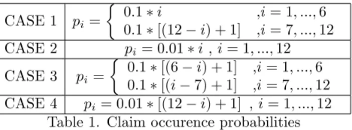
C O M PO U N D BIN O M IA L R ISK M O D EL W IT H D ISC R ET E PH A SE-T Y PE C LA IM S 15 This distribution given by Eq. (3.1) is known to be geometric distribution of order "2" Eryilmaz [7]. Let de…ne cases with non-homogenous claim occurrence proba-bilities in each periods as follows:

CASE 1 pi = 0:1 i ,i = 1; :::; 6 0:1 [(12 i) + 1] ,i = 7; :::; 12 CASE 2 pi= 0:01 i , i = 1; :::; 12 CASE 3 pi= 0:1 [(6 i) + 1] ,i = 1; :::; 6 0:1 [(i 7) + 1] ,i = 7; :::; 12 CASE 4 pi= 0:01 [(12 i) + 1] , i = 1; :::; 12

Table 1. Claim occurence probabilities

In Case 1, it can be seen that the probabilities of claim occurrences are increasing for …rst 6 periods from 0:1 to 0:6 and after that it is decreasing for last 6 periods from 0:6 to 0:1. In Case 2, it can be seen that the probabilities of claim occurrences are increasing from 0:01 to 0:12 for 12 periods. In Case 3, probabilities of claim occurrences are decreasing for …rst 6 periods from 0:6 to 0:1 and after that it is increasing for last 6 periods from 0:1 to 0:6. Finally, in Case 4, the probabilities of claim occurrences are decreasing from 0:12 to 0:01 for 12 periods.

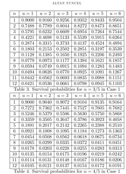
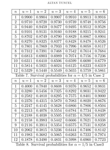
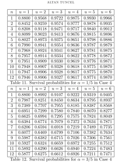
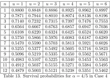
So, survival probabilities are calculated and presented in Table 2 - Table 13 for di¤erent values, which are probability of claims, by Eq. (1.10) when P (Ii= 1) = pifor i = 1; 2; : : : ; 12. n u = 1 u = 2 u = 3 u = 4 u = 5 u = 6 1 0:9000 0:9640 0:9768 0:9896 0:9942 0:9972 2 0:8352 0:9094 0:9509 0:9727 0:9854 0:9920 3 0:7505 0:8621 0:9139 0:9512 0:9710 0:9835 4 0:6870 0:7966 0:8720 0:9187 0:9502 0:9692 5 0:5995 0:7321 0:8124 0:8766 0:9177 0:9470 6 0:5238 0:6431 0:7435 0:8152 0:8720 0:9114 7 0:4363 0:5661 0:6624 0:7490 0:8140 0:8664 8 0:3845 0:4990 0:6021 0:6887 0:7629 0:8219 9 0:3464 0:4598 0:5576 0:6475 0:7234 0:7877 10 0:3271 0:4347 0:5323 0:6209 0:6986 0:7646 11 0:3168 0:4229 0:5189 0:6075 0:6853 0:7523 12 0:3134 0:4186 0:5142 0:6025 0:6805 0:7477

(20)

16 A LTA N T U N C EL n u = 1 u = 2 u = 3 u = 4 u = 5 u = 6 1 0:9000 0:9160 0:9256 0:9352 0:9433 0:9504 2 0:7488 0:7789 0:8044 0:8272 0:8473 0:8651 3 0:5795 0:6232 0:6609 0:6954 0:7264 0:7544 4 0:4221 0:4698 0:5133 0:5539 0:5915 0:6264 5 0:2874 0:3315 0:3733 0:4137 0:4524 0:4894 6 0:1803 0:2153 0:2502 0:2851 0:3197 0:3539 7 0:1128 0:1385 0:1650 0:1925 0:2206 0:2493 8 0:0779 0:0973 0:1177 0:1394 0:1621 0:1857 9 0:0594 0:0749 0:0915 0:1094 0:1283 0:1483 10 0:0494 0:0626 0:0770 0:0925 0:1091 0:1267 11 0:0442 0:0562 0:0693 0:0835 0:0988 0:1151 12 0:0421 0:0536 0:0661 0:0798 0:0945 0:1103

Table 3. Survival probabilities for = 3=5 in Case 1

n u = 1 u = 2 u = 3 u = 4 u = 5 u = 6 1 0:9000 0:9040 0:9072 0:9104 0:9135 0:9164 2 0:7272 0:7362 0:7445 0:7527 0:7605 0:7682 3 0:5246 0:5379 0:5506 0:5630 0:5750 0:5868 4 0:3359 0:3505 0:3647 0:3786 0:3923 0:4058 5 0:1891 0:2017 0:2142 0:2265 0:2388 0:2510 6 0:0921 0:1008 0:1095 0:1184 0:1273 0:1363 7 0:0454 0:0508 0:0562 0:0618 0:0675 0:0734 8 0:0265 0:0299 0:0335 0:0372 0:0411 0:0451 9 0:0178 0:0203 0:0228 0:0255 0:0283 0:0313 10 0:0135 0:0154 0:0175 0:0196 0:0219 0:0242 11 0:0114 0:0131 0:0148 0:0167 0:0186 0:0206 12 0:0105 0:0121 0:0137 0:0154 0:0172 0:0191

(21)

C O M PO U N D BIN O M IA L R ISK M O D EL W IT H D ISC R ET E PH A SE-T Y PE C LA IM S 17 n u = 1 u = 2 u = 3 u = 4 u = 5 u = 6 1 0:9900 0:9964 0:9977 0:9990 0:9994 0:9997 2 0:9829 0:9917 0:9955 0:9977 0:9988 0:9994 3 0:9757 0:9884 0:9936 0:9968 0:9983 0:9991 4 0:9712 0:9856 0:9922 0:9959 0:9978 0:9958 5 0:9676 0:9836 0:9910 0:9953 0:9975 0:9987 6 0:9650 0:9820 0:9900 0:9947 0:9971 0:9985 7 0:9629 0:9807 0:9893 0:9943 0:9969 0:9983 8 0:9612 0:9796 0:9886 0:9938 0:9966 0:9981 9 0:9598 0:9787 0:9880 0:9935 0:9964 0:9980 10 0:9586 0:9779 0:9875 0:9931 0:9962 0:9979 11 0:9525 0:9772 0:9870 0:9928 0:9960 0:9977 12 0:9566 0:9765 0:9865 0:9925 0:9958 0:9976

n u = 1 u = 2 u = 3 u = 4 u = 5 u = 6 1 0:9900 0:9916 0:9926 0:9935 0:9943 0:9950 2 0:9734 0:9768 0:9797 0:9822 0:9844 0:9864 3 0:9516 0:9578 0:9629 0:9675 0:9715 0:9750 4 0:9269 0:9359 0:9436 0:9505 0:9565 0:9617 5 0:9003 0:9123 0:9226 0:9318 0:9399 0:9470 6 0:8729 0:8877 0:9007 0:9122 0:9223 0:9313 7 0:8452 0:8628 0:8782 0:8919 0:9040 0:9148 8 0:8178 0:8377 0:8553 0:8711 0:8852 0:8977 9 0:7906 0:8128 0:8324 0:8500 0:8658 0:8800 10 0:7639 0:7879 0:8093 0:8287 0:8461 0:8617 11 0:7376 0:7632 0:7862 0:8070 0:8259 0:8430 12 0:7117 0:7386 0:7629 0:7851 0:8053 0:8236

(22)

n u = 1 u = 2 u = 3 u = 4 u = 5 u = 6 1 0:4000 0:7840 0:8608 0:9376 0:9652 0:9831 2 0:3280 0:5456 0:7325 0:8292 0:9031 0:9422 3 0:2582 0:4810 0:6295 0:7575 0:8401 0:9000 4 0:2376 0:4315 0:5870 0:7083 0:8020 0:8676 5 0:2247 0:4145 0:5628 0:6866 0:7806 0:8504 6 0:2213 0:4076 0:5554 0:6784 0:7734 0:8438 7 0:2188 0:4038 0:5505 0:6735 0:7685 0:8397 8 0:2158 0:3983 0:5442 0:6666 0:7621 0:8338 9 0:2116 0:3914 0:5354 0:6575 0:7531 0:8258 10 0:2062 0:3815 0:5236 0:6444 0:7406 0:8142 11 0:1983 0:3682 0:5065 0:6263 0:7222 0:7974 12 0:1878 0:3490 0:4831 0:5998 0:6960 0:7723

(23)

n u = 1 u = 2 u = 3 u = 4 u = 5 u = 6 1 0:4000 0:4240 0:4432 0:4624 0:4808 0:4986 2 0:2080 0:2264 0:2429 0:2594 0:2756 0:2916 3 0:1306 0:1445 0:1573 0:1703 0:1833 0:1962 4 0:0952 0:1064 0:1169 0:1275 0:1383 0:1490 5 0:0786 0:0882 0:0974 0:1067 0:1162 0:1257 6 0:0719 0:0809 0:0895 0:0983 0:1071 0:1161 7 0:0660 0:0744 0:0825 0:0907 0:0991 0:1075 8 0:0555 0:0629 0:0699 0:0772 0:0846 0:0921 9 0:0426 0:0486 0:0544 0:0603 0:0664 0:0726 10 0:0297 0:0341 0:0385 0:0430 0:0476 0:0524 11 0:0185 0:0215 0:0245 0:0276 0:0308 0:0342 12 0:0102 0:0119 0:0137 0:0137 0:0176 0:0197

(24)

n u = 1 u = 2 u = 3 u = 4 u = 5 u = 6 1 0:8800 0:8992 0:9107 0:9222 0:9319 0:9405 2 0:7987 0:8251 0:8450 0:8634 0:8795 0:8937 3 0:7389 0:7707 0:7955 0:8185 0:8387 0:8568 4 0:6951 0:7299 0:7580 0:7840 0:8070 0:8277 5 0:6625 0:6994 0:7295 0:7575 0:7824 0:8049 6 0:6384 0:6774 0:7079 0:7372 0:7634 0:7871 7 0:6206 0:6594 0:6918 0:7219 0:7489 0:7735 8 0:6077 0:6469 0:6799 0:7106 0:7382 0:7634 9 0:5987 0:6382 0:6715 0:7026 0:7306 0:7561 10 0:5927 0:6324 0:6659 0:6972 0:7255 0:7512 11 0:5892 0:6290 0:6626 0:6940 0:7224 0:7483 12 0:5877 0:6275 0:6612 0:6926 0:7211 0:7471

(25)

In case of nonhomogenous claim occurence probabilities, it is obvious to say that the survival probabilities are increasing when the u initial values are increasing and survival probabilities are decreasing for same u initial reserve level in later periods. It is also possible to see that the survival probabilities are decreasing for higher values of for each cases. Survival probabilities are decreasing for higher probablities of claim occurence with same level which can be seen by comparing the Tables are given for Case 2 and Case 4. Similar interpretations can be made for Case 1 and Case 3.

4. Conclusion

The theoretical assumptions of this study are basically taken from Tank and Tun-cel [17]. In this study, survival exact probabilities in compound binomial risk model are calculated with nonhomogeneous probabilities where the individual claim sizes are discrete Phase Type distribution instead of geometric distribution. Probabilites are calculated by MATLAB software where the individual claim size distribution is discrete phase type distribution and presented in Tables 2-13. By using the given probablities it is easy to calculate the ruin probabilities for an insurance company with respect to the parameters which are assumed.

As a possible future work, nonruin (survival) probabilities for dependent case of Ii(i 1) and continuous time compound binomial risk model can also be studied.

References

[1] Asmussen, S., 2000. Ruin probabilities. World Scienti…c, Singapore.

[2] Bladt, M. 2005. A review on phase-type distributions and their use in risk theory. Astin Bulletin, 35(01), 145-161.

[3] Breuer, L., and Baum, D. 2005. Phase-Type Distributions. An Introduction to Queueing Theory and Matrix-Analytic Methods, 169-184.

(26)

[4] Chen, X. H., Dempster, A. P., and Liu, J. S. 1994. Weighted …nite population sampling to maximize entropy. Biometrika, 81(3), 457-469.

[5] Dickson, D. C. 1994. Some comments on the compound binomial model. Astin Bulletin, 24(01), 33-45.

[6] Drekic, S. 2006. Phase-Type Distribution. Encyclopedia of Quantitative Finance.

[7] Eryilmaz S., 2014. On distributions of runs in the compound binomial risk model, Methodol. Comput. Appl. Probab. 16 (1).149-159.

[8] Gerber, H. U. 1988. Mathematical fun with the compound binomial process. Astin Bulletin, 18(02), 161-168.

[9] Latouche, G., Ramaswami, V., 1999. Introduction to matrix analytic methods in stochastic modeling. ASA SIAM, Philadelphia

[10] Li, S., and Sendova, K. P. 2013. The …nite-time ruin probability under the compound binomial risk model. European Actuarial Journal, 3(1), 249-271.

[11] Liu, G., Wang, Y., and Zhang, B. 2005. Ruin probability in the continuous-time compound binomial model. Insurance: Mathematics and Economics, 36(3), 303-316.

[12] Liu, G., and Zhao, J. 2007. Joint distributions of some actuarial random vectors in the compound binomial model. Insurance: Mathematics and Economics, 40(1), 95-103.

[13] Neuts, M.F., 1975. Probability distributions of phase type. University of Louvain, pp. 173-206. [14] Neuts, M.F., 1981. Matrix-geometric solutions in stochastic models: An algorithmic

ap-proach.Johns Hopkins University Press, Baltimore.

[15] Stanford, D.A., Stroinski, K.J., 1994. Recursive methods for computing …nite-time ruin prob-abilities for phase-distributed claim sizes. ASTIN Bull. 24, 235-254.

[16] Shiu, E. S. 1989. The probability of eventual ruin in the compound binomial model. Astin Bulletin, 19(2), 179-190.

[17] Tank, F., and Tuncel, A. 2015. Some results on the extreme distributions of surplus process with nonhomogeneous claim occurrences. Hacettepe Journual of Mathematics and Statistics 44(2), 475-484.

[18] Tank, F., and Eryilmaz, S. 2015. The distributions of sum, minima and maxima of generalized geometric random variables. Statistical Papers 56(4), 1191-1203.

[19] Tuncel, A., and Tank, F. 2014. Computational results on the compound binomial risk model with nonhomogeneous claim occurrences. Journal of Computational and Applied Mathemat-ics, 263, 69-77.

[20] Willmot, G. E. 1993. Ruin probabilities in the compound binomial model. Insurance: Math-ematics and Economics, 12(2), 133-142.

[21] Wu, X. and Li, S., 2008. On a discrete-time Sparre Anderson model with phase-type claims, Working paper 08-169, Department of Economics, 1–16. University of Melbourne, http://www.mercury.ecom.unimelb.edu.au/SITE/actwww/wps2008/No169.pdf.

Current address : Altan TUNCEL: Kirikkale University, Faculty of Arts and Sciences, Depart-ment of Actuarial Sciences, Yahsihan- Kirikkale, TURKEY

(27)

C o m m u n . Fa c . S c i. U n iv . A n k . S é r. A 1 M a t h . S ta t . Vo lu m e 6 5 , N u m b e r 2 , P a g e s 2 3 –3 6 (2 0 1 6 ) D O I: 1 0 .1 5 0 1 / C o m m u a 1 _ 0 0 0 0 0 0 0 7 5 6 IS S N 1 3 0 3 –5 9 9 1

INVERSE NODAL PROBLEM FOR p LAPLACIAN DIFFUSION

EQUATION WITH POLYNOMIALLY DEPENDENT SPECTRAL PARAMETER

TUBA GULSEN AND EMRAH YILMAZ

Abstract. In this study, solution of inverse nodal problem for one-dimensional p-Laplacian di¤usion equation is extended to the case that boundary condi-tion depends on polynomial eigenparameter. To …nd the spectral datas as eigenvalues and nodal parameters of this problem, we used a modi…ed Prüfer substitution. Then, reconstruction formula of the potential function is also given by using nodal lenghts. Furthermore, this method is similar to used in [1], our results are more general.

(Dedicated to Prof. E. S. Panakhov on his 60-th birthday)

1. Introduction

Let us consider following p Laplacian di¤usion eigenvalue problem [1]

y0(p 1) 0= (p 1) 2 qm(x) 2 rm(x) y(p 1); 0 x 1; (1.1)

with the boundary conditions

y(0) = 0; y0(0) = 1;

y0(1; ) + f ( )y(1; ) = 0; (1.2)

where p > 1 is a constant, [2]

f ( ) = a1 + a2 2+ ::: + am m; ai2 R; am6= 0; m 2 Z+; (1.3) is a spectral parameter and y(p 1)_{= jyj}(p 2)_{y: Throughout this study, we suppose} that qm(x) 2 L2(0; 1) and rm(x) 2 W21(0; 1) are real-valued functions de…ned in the interval 0 x _{1 for all m 2 Z}+. Equation (1.1) becomes following well-known di¤usion equation (or quadratic pencil of di¤erential pencil)

y00+ [qm+ 2 rm] y = 2y; (1.4)

Received by the editors: February 09, 2016, Accepted: April 27, 2016. 2010 Mathematics Subject Classi…cation. 34A55, 34L05, 34L20.

Key words and phrases. Inverse Nodal Problem, Prüfer Substitution, Di¤usion equation.

c 2 0 1 6 A n ka ra U n ive rsity C o m m u n ic a tio n s d e la Fa c u lté d e s S c ie n c e s d e l’U n ive rs ité d ’A n ka ra . S é rie s A 1 . M a th e m a t ic s a n d S t a tis t ic s .

(28)

24 T U BA G U LSEN A N D EM R A H Y ILM A Z

for p = 2: Equation (1.4) is extremely important for both classical and quantum mechanics. For instance, such problems arise in solving the Klein-Gordon equations, which describe the motion of massless particles such as photons. Di¤usion equations are also used for modelling vibrations of mechanical systems in viscous media (see [3]). We note that in this type of problem the spectral parameter is related to the energy of the system, and this motivates the terminology ‘energy-dependent’used for the spectral problem of the form (1.4). Inverse problems of quadratic pencil have been studied by numerous authors (see [4], [5], [6], [7], [8], [9], [10], [11], [12], [13], [14], [15], [16], [17], [18], [19], [20]).

Inverse spectral problem consists in recovering di¤erential equation from its spec-tral parameters like eigenvalues, norming constants and nodal points (zeros of eigen-functions). These type problems divide into two parts as inverse eigenvalue problem and inverse nodal problem. They play important role and also have many appli-cations in applied mathematics. Inverse nodal problem has been …rstly studied by McLaughlin in 1988. She showed that the knowledge of a dense subset of nodal points is su¢ cient to determine the potential function of Sturm-Liouville problem up to a constant [21]. Also, some numerical results about this problem were given in [22]. Nowadays, many authors have given some interesting results about inverse nodal problems for di¤erent type operators (see [23], [24], [25], [26], [27]).

In this study, we concern ourselves with the inverse nodal problem for p Laplacian di¤usion equation with boundary condition polynomially dependent on spectral pa-rameter. As far as we know, this problem has not been considered before. Fur-thermore, we give asymptotics of eigenparameters and reconstructing formula for potential function. Note that inverse eigenvalue problems for di¤erent p Laplacian operators have been studied by several authors (see [28], [29], [30], [31], [32], [33], [34], [35], [36]).

The zero set Xn = xnj;m n 1

j=1 of the eigenfunction yn;m(x; ) corresponding to n;m is called the set of nodal points where 0 = x(n)0;m < x

(n)

1;m < ::: < x (n) n 1;m < x(n)n;m= 1 for all m 2 Z+: And, lnj;m= xnj+1;m xnj;mis referred to the nodal length of yn;m: The eigenfunction yn;m(x) has exactly n 1 nodal points in (0; 1):

Firstly, we need to introduce generalized sine function Sp which is the solution of the initial value problem

S_p0(p 1) 0 = (p 1)S(p 1)_p ; (1.4)

Sp(0) = 0; Sp0(0) = 1: Sp and Sp0 are periodic functions satisfying the identity

jSp(x)jp+ Sp0(x) p

= 1;

for arbitrary x 2 R: These functions are p analogues of classical sine and cosine functions and are known as generalized sine and cosine functions. It is well known

(29)

IN V ER SE N O DA L PRO BLEM FO R p LA PLAC IA N D IFFU SIO N EQ U AT IO N 25 that ^ = 1 Z 0 2 (1 tp₎1p dt = 2 p sin _p ;

is the …rst zero of Sp in positive axis (See [28], [29]): Note that following lemma is crucial in our results.

Lemma 1.1.

[28] a)For S0 p6= 0; S_p0 0 = Sp S0 p p 2 Sp: b) SpS 0_{(p 1)} p 0 = S_p0 p (p 1) S_pp = 1 _{p jS}pjp= (1 p) + p Sp0 p : Using Sp(x) and S0p(x); the generalized tangent function Tp(x) can be de…ned by [28] Tp(x) = Sp(x) S0 p(x); for x 6= k + 1 2 ^:

This study is organized as follows: In Section 2, we give some asymptotic formu-las for eigenvalues and nodal parameters for p Laplacian di¤usion eigenvalue prob-lem (1.1)-(1.2) with polynomially dependent spectral parameter by using modi…ed Prüfer substitution. In Section 3, we give a reconstruction formula of the potential functions for the problem (1.1)-(1.2). Finally, we expressed some conclusions in Section 4.

2. Asymptotics of Some Eigenparameters

In this section, we present some important results for the problem (1.1)-(1.2). To do this, we need to consider modi…ed Prüfer’s transformation which is one of the most powerful method for solution of inverse problem. Recalling that Prüfer’s transformation for a nonzero solution y of (1.1) takes the form

y(x) = R(x)Sp 2=p (x; ) ; (2.1) y0(x) = 2=pR(x)S0_p 2=p (x; ) ; or y0_(x) y(x) = 2=pS 0 p 2=p (x; ) Sp 2=p (x; ) ; (2.2)

(30)

where R(x) is amplitude and (x) is Prüfer variable [37]. After some straightforward computations, one can get easily [1]

0_{(x; ) = 1} qm(x) 2 S p p 2=p (x; ) 2 rm(x)Spp 2=p (x; ) : (2.3)

Lemma 2.1.

[30] De…ne (x; n;m) as in (2.1) and n(x) = Spp 2=pn;m (x; n;m) 1

p: Then, for any g 2 L 1_{(0; 1)}

1 Z 0

n(x)g(x)dx = 0:

Theorem 2.1.

The eigenvalues n;m of the p Laplacian di¤ usion eigenvalue problem given in (1.1)-(1.2) have the form

2=p n;1 = n^ 1 a1(n^) p 2 2 + 1 p (n^)p 1 1 Z 0 q1(x)dx + 2 p (n^)p22 1 Z 0 r1(x)dx + O 1 np 2 ; (2.4) 2=p n;2 = n^ 1 a1(n^) p 2 2 _{+ a} 2(n^)p 1 + 1 p (n^)p 1 1 Z 0 q2(x)dx + 2 p (n^)p22 1 Z 0 r2(x)dx + O 1 np 1 ; (2.5) 2=p n;m = n^ 1 a1(n^) p 2 2 _{+ ::: + a} m(n^) mp 2 2 + 1 p (n^)p 1 1 Z 0 qm(x)dx + 2 p (n^)p22 1 Z 0 rm(x)dx + O 1 np 1 ; (2.6)

for m = 1; m = 2 and m _{3; respectively as n ! 1.}

Proof:

Let (0; ) = 0 for the problem (1.1)-(1.2). Integrating both sides of (2.3) with respect to x from 0 to 1, we get

(1; ) = 1 1₂ 1 Z 0 qm(x)Spp 2=p (x; ) dx 2Z1 0 rm(x)Spp 2=p (x; ) dx:

(31)

IN V ER SE N O DA L PRO BLEM FO R p LA PLAC IA N D IFFU SIO N EQ U AT IO N 27 By lemma 2.1, one can obtain

1 Z 0 qm(x) Spp 2=p n (x; ) 1 p dx = o(1); as n ! 1: Hence, we obtain 2=p (1; ) = 2=p 1 p 2 2p 1 Z 0 qm(x)dx 2 p 1 2p 1 Z 0 rm(x)dx + O 1 2 2 p : (2.7)

Let n;m be an eigenvalue of the problem (1.1)-(1.2) for all m. Now, we will prove the lemma for m = 1. By (1.2), we have

2=p n;1R(1)Sp0 2=p n;1 (1; n;1) + a1 n;1R(1)Sp 2=pn;1 (1; n;1) = 0; or 2 p 1 n;1 a1 = Sp 2=pn;1 (1; n;1) S0 p 2=p n;1 (1; n;1) = Tp 2=pn;1 (1; n;1) : As n is su¢ ciently large, it follows

2=p n;1 (1; n;1) = Tp 1 0 @ 2 p 1 n;1 a1 1 A = n^ 2 p 1 n;1 a1 + o 4 p 2 n;1 : (2.8)

By considering (2.7) and (2.8) together, we get 2=p n;1 = n^ 1 a1(n^) p 2 2 + 1 p (n^)p 1 1 Z 0 q1(x)dx + 2 p (n^)p22 1 Z 0 r1(x)dx + O 1 np 2 : For the case m = 2, by using the similar process as in m = 1, we can easily obtain

2=p n;2R(1)Sp0 2=p n;2 (1; n;2) + a1 n;2+ a2 2n;2 R(1)Sp 2=pn;2 (1; n;2) = 0; or 2 p n;2 a1 n;2+ a2 2n;2 = Sp 2=pn;2 (1; n;2) S0 p 2=p n;2 (1; n;2) = Tp 2=pn;2 (1; n;2) ; and 2=p n;2 (1; n;2) = n^ 2 p n;2 a1 n;2+ a2 2n;2 + o 0 @ 4 p n;2 a1 n;2+ a2 2n;2 2 1 A : (2.9)

(32)

28 T U BA G U LSEN A N D EM R A H Y ILM A Z Therefore, we have 2=p n;2 = n^ 1 a1(n^) p 2 2 _{+ a} 2(n^)p 1 + 1 p (n^)p 1 1 Z 0 q2(x)dx + 2 p (n^)p22 1 Z 0 r2(x)dx + O 1 np 1 ;

by using (2.7) and (2.9). Finally, let us …nd the asymptotic expansion of n;mfor m 3: Similarly, by using (1.2), we have

2=p n;mR(1)Sp0 2=p n;m (1; n;m) + a1 n;m+ ::: + am mn;m R(1)Sp 2=pn;m (1; n;m) = 0; or 2 p n;m a1 n;m+ ::: + am mn;m = Sp 2=pn;m (1; n;m) S0 p 2=pn;m (1; n;m) = Tp 2=pn;m (1; n;m) : (2.10)

By considering (2.7) and (2.10) together and using similar procedure, we deduce that 2=p n;m = n^ 1 a1(n^) p 2 2 _{+ ::: + a} m(n^) mp 2 2 + 1 p (n^)p 1 1 Z 0 qm(x)dx + 2 p (n^)p22 1 Z 0 rm(x)dx + O 1 np 1 :

Theorem 2.2.

Asymptotic estimates of the nodal points for the problem (1.1)-(1.2) satis…es xn_j;1= j n j a1n p+2 2 ^ p 2 + j pnp+1_^p 1 Z 0 q1(t)dt + 2j pnp2+1^ p 2 1 Z 0 r1(t)dt + 1 (n^)p xn j;1 Z 0 q1(t)Sppdt + 2 (n^)p2 xn j;1 Z 0 r1(t)Sppdt + O j np ; (2.11)

(33)

IN V ER SE N O DA L PRO BLEM FO R p LA PLAC IA N D IFFU SIO N EQ U AT IO N 29 xn_j;2 = j n j a1n p+2 2 ^ p 2 + a 2np^p + j pnp+1_^p 1 Z 0 q2(t)dt + 2j pnp2+1^ p 2 1 Z 0 r2(t)dt + 1 (n^)p xn j;2 Z 0 q2(t)Sppdt + 2 (n^)p2 xn j;2 Z 0 r2(t)Sppdt + O j np+1 ; (2.12) and xn_j;m = j n j a1n p+2 2 ^ p 2 _{+ ::: + a} mn mp 2 +1^ mp 2 + j pnp+1_^p 1 Z 0 qm(t)dt + 2j pnp2+1^ p 2 1 Z 0 rm(t)dt + 1 (n^)p xZnj;m 0 qm(t)Sppdt + 2 (n^)p2 xn j;m Z 0 rm(t)Sppdt + O j np+1 ; (2.13)

Proof:

Integrating (2.3) from 0 to xn_j;m and letting (xn_j;m; ) = j ^_2=p n;m ; we have xn_j;m= j ^_2=p n;m + ₂1 n;m xZnj;m 0 qm(t)Sppdt + 2 n;m xZnj;m 0 rm(t)Sppdt: (2.14) Now, we will …nd the asymptotic estimate of nodal points for m = 1. From the formula (2.4), we deduce 1 2=p n;1 = 1 n^ 1 a1(n^) p+2 2 + 1 p (n^)p+1 1 Z 0 q1(t)dt + 2 p (n^)p2+1 1 Z 0 r1(t)dt + O 1 np ; (2.15) and therefore we obtain the formula (2.11) by using (2.14) and (2.15).

In (2.11), if we take j n ! 1 as n ! 1, we obtain xn_j;1= j n j a1n p+2 2 ^ p 2 + j pnp+1_^p 1 Z 0 q1(t)dt + 2j pnp2+1^ p 2 1 Z 0 r1(t)dt + 1 p (n^)p 1 Z 0 q1(t)dt + 2 p (n^)p2 1 Z 0 r1(t)dt + O 1 np2+1 : (2.16)

(34)

By using (2.5), the asymptotic estimate of eigenvalues 1= 2=p_n;2 for m = 2 is considered as 1 2=p n;2 = 1 n^ 1 a1(n^) p+2 2 _{+ a} 2(n^)p+1 + 1 p (n^)p+1 1 Z 0 q2(t)dt + 2 p (n^)p2+1 1 Z 0 r2(t)dt + O 1 np+1 ; (2.17)

and, we conclude the formula (2.12) by using (2.14) and (2.17). In the formula (2.12), if we take j

n ! 1 as n ! 1, we have xn_j;2= j n j a1n p+2 2 ^ p 2 _{+ a} 2np^p + j pnp+1_^p 1 Z 0 q2(t)dt + 2j pnp2+1^ p 2 1 Z 0 r2(t)dt + 1 p (n^)p 1 Z 0 q2(t)dt + 2 p (n^)p2 1 Z 0 r2(t)dt + O 1 np2+1 : (2.18)

For m 3, from the formula (2.6), it can be easily obtain that 1 2=p n;m = 1 n^ 1 a1(n^) p+2 2 _{+ ::: + a} m(n^) mp+2 2 + 1 p (n^)p+1 1 Z 0 qm(t)dt + 2 p (n^)p2+1 1 Z 0 rm(t)dt + O 1 np+1 ; (2.19)

and we get the formula (2.13) by using (2.14) and (2.19). In (2.13), if we take j n ! 1 as n ! 1, we obtain xn_j;m= j n j a1n p+2 2 ^ p 2 + ::: + a mn mp 2 +1^ mp 2 + j pnp+1_^p 1 Z 0 qm(t)dt + 2j pnp2+1^ p 2 1 Z 0 rm(t)dt + 1 p (n^)p 1 Z 0 qm(t)dt + 2 p (n^)p2 1 Z 0 rm(t)dt + O 1 np2+1 : (2.20)

(35)

IN V ER SE N O DA L PRO BLEM FO R p LA PLAC IA N D IFFU SIO N EQ U AT IO N 31

Theorem 2.3.

Asymptotic estimate of the nodal lengths for the problem (1.1)-(1.2) satis…es ln_j;1= 1 n 1 a1n p+2 2 ^ p 2 + 1 pnp+1_^p 1 Z 0 q1(t)dt + 2 pnp2+1^ p 2 1 Z 0 r1(t)dt (2.21) + 1 (n^)p xZnj+1;1 xn j;1 q1(t)Sppdt + 2 (n^)p2 xZnj+1;1 xn j;1 r1(t)Sppdt + O 1 np ; ln_j;2= 1 n 1 a1n p+2 2 ^ p 2 _{+ a} 2np+1^p + 1 pnp+1_^p 1 Z 0 q2(t)dt + 2 pnp2+1^ p 2 1 Z 0 r2(t)dt (2.22) + 1 (n^)p xn j+1;2 Z xn j;2 q2(t)Sppdt + 2 (n^)p2 xn j+1;2 Z xn j;2 r2(t)Sppdt + O 1 np+1 ; and ln_j;m= 1 n 1 a1n p+2 2 ^ p 2 _{+ ::: + a} mn mp 2 +1^ mp 2 + 1 pnp+1_^p 1 Z 0 qm(t)dt + 2 pnp2+1^ p 2 1 Z 0 rm(t)dt + 1 (n^)p xnj+1;mZ xn j;m qm(t)Sppdt + 2 (n^)p2 xnj+1;mZ xn j;m rm(t)Sppdt + O 1 np+1 ; (2.23)

Proof:

_{For large n 2 N, integrating (2.3) in [x}n

j;m; xnj+1;m] and using the de…nition

of nodal lengths, we have

ln_j;m= _2=p^ n;m + ₂1 n;m xnj+1;mZ xn j;m qm(t)Sppdt + 2 n;m xnj+1;mZ xn j;m rm(t)Sppdt; (2.24) or

(36)

32 T U BA G U LSEN A N D EM R A H Y ILM A Z l_j;mn = ^ 2=p n;m + 1 p 2_n;m xn j+1;mZ xn j;m qm(t)dt + 2 p n;m xn j+1;mZ xn j;m rm(t)dt + O 1 np2+1 :

For m = 1, m = 2 and m 3, we can obtain easily (2.21), (2.22) and (2.23) by using the formulas (2.15), (2.17), (2.19), respectively.

3. Reconstruction of the potential function

In this section, we give an explicit formula for the potential functions of the di¤usion equation (1.1) by using nodal lengths. The method used in the proof of the theorem is similar to classical problems; p Laplacian Sturm-Liouville eigenvalue problem and p Laplacian energy-dependent Sturm-Liouville eigenvalue problem (see [1], [29], [30], [31]).

Theorem 3.1.

Let qm(x) 2 L2(0; 1) and rm(x) 2 W21(0; 1) are real-valued func-tions de…ned in the interval 0 x 1 for all m: Then

qm(x) = lim n!1 0 @p 2 p+2 n;mlnj;m ^ p 2 n;m 1 A ; (2.25) and rm(x) = lim n!1 0 @p 2 p+1 n;mlj;mn 2^ p n;m 2 1 A ; for j = jn;m(x) = max j : xnj;m< x and m 2 Z+.

Proof:

We need to consider Theorem 2.3 for proof. From (2.24), we have p 2=p+2_n;m ^ l n j;m= p 2 n;m+ p 2=p_n;m ^ xnj+1;mZ xn j;m qm(t)Sppdt + 2p 2=p+1_n;m ^ xnj+1;mZ xn j;m rm(t)Sppdt:

Then, we can use similar procedure as those in [29] for j = jn;m(x) = maxfj : xn_j;m_{< xg to show} 2=p n;m ^ xnj+1;mZ xn j;m qm(t)dt ! qm(x); and p 2=p_n;m ^ xn j+1;mZ xn j;m qm(t) Spp 1 p dt ! 0;

(37)

IN V ER SE N O DA L PRO BLEM FO R p LA PLAC IA N D IFFU SIO N EQ U AT IO N 33 pointwise almost everywhere. Hence, we get

qm(x) = lim n!1 0 @p 2 p+2 n;mlnj;m ^ p 2 n;m 1 A :

By using similar way, we can easily get the asymptotic expansion of rm(x):

Theorem 3.2.

Let n

l(n)_j;m: j = 1; 2; :::; n 1 o₁

n=2be a set of nodal lengths of the problem (1.1)-(1.2) where qm(x) and rm(x) are real-valued functions on 0 x 1 for all m. Let us de…ne

Fn;1(x) = p (n^)p nlj;1(n) 1 p a1 (n^)p=2+ 1 Z 0 q1(t)dt+2 (n^)p=2 1 Z 0 r1(t)dt; (2.26) Fn;2(x) = p (n^)p nl(n)j;2 1 p (n^)p=2 a1+ a2(n^)p=2 + 1 Z 0 q2(t)dt + 2 (n^)p=2 1 Z 0 r2(t)dt; (2.27) Fn;m(x) = p (n^)p nl(n)j;m 1 p (n^)p=2 a1+ ::: + am(n^) mp p 2 + 1 Z 0 qm(t)dt + 2 (n^)p=2 1 Z 0 rm(t)dt: (2.28) and Gn;1(x) = p (n^)p2 2 nl (n) j;1 1 p 2a1 + 1 2 (n^)p=2 1 Z 0 q1(t)dt + 1 Z 0 r1(t)dt; (2.29) Gn;2(x) = p (n^)p2 2 nl (n) j;2 1 p 2 a1+ a2(n^) p 2 + 1 2 (n^)p=2 1 Z 0 q2(t)dt + 1 Z 0 r2(t)dt (2.30)

(38)

34 T U BA G U LSEN A N D EM R A H Y ILM A Z Gn;m(x) = p (n^)p2 2 nl (n) j;m 1 p 2 a1+ ::: + am(n^) mp p 2 + 1 2 (n^)p2 1 Z 0 qm(t)dt + 1 Z 0 rm(t)dt (2.31)

for m = 1; m = 2 and m _{3; respectively. Then, fF}n;m(x)g and fGn;m(x)g converge to qmand rmpointwise almost everywhere in L1(0; 1); respectively, for all cases.

Proof:

We will prove this theorem only for Fn;1. Other cases can be shown similarly. By the asymptotic formulas of eigenvalues (2.4) and nodal lengths (2.21), we get p 2_n;1 2=p n;1lnj;1 ^ 1 ! = p 2_n;1 nl(n)_j;1 1 p a1 (n^)p=2+1l(n)_j;1 + nl_j;1(n) 1 Z 0 q1(t)dt + 2n (n^)p=2l(n)_j;1 1 Z 0 r1(t)dt + o(1):

Considering nl(n)_j;1 _{= 1 + o(1); as n ! 1, we have} p (n^)p nl_j;1(n) 1 p a1 (n^)p=2 _{! q}1(x) 1 Z 0 q1(t)dt 2 (n^)p=2 1 Z 0 r1(t)dt pointwise almost everywhere in L1_{(0; 1): By using similar way, it is not di¢ cult} to show that fGn;m(x)g converges to rm pointwise almost everywhere in L1(0; 1); respectively, for all m 2 Z+_:

4. Conclusion

In this study, we give some asymptotic estimates for eigenvalues, nodal parame-ters and potential function of the p Laplacian di¤usion eigenvalue problem (1.1)-(1.2) with polynomially dependent spectral parameter. We show that the obtained results are generalizations of the classical problem.

References

[1] Koyunbakan, H. 2013. Inverse nodal problem for p Laplacian energy-dependent Sturm-Liouville equation, Boundary Value Problems 2013:272 (Erratum: Inverse nodal problem for p Laplacian energy-dependent Sturm-Liouville equation, Boundary Value Problems, 2014:222 (2014).

[2] Yang, C.F. and Yang, X. 2011. Ambarzumyan’s theorem with eigenparameter in the boundary conditions, Acta Mathematica Scientia 31(4), 1561-1568.