DOI: 10.18869/acadpub.jafm.73.238.26166
Experimental and Numerical Investigation of a Longfin
Inshore Squid’s Flow Characteristics
A. Bahadir Olcay
1†, M. Tabatabaei Malazi
2, A. Okbaz
2, H. Heperkan
2, E. Firat
3, V.
Ozbolat
3, M. Gokhan Gokcen
4and B. Sahin
31Yeditepe University, Mechanical Engineering Department, Atasehir, Istanbul 34755, Turkey 2Yildiz Technical University, Faculty of Mechanical Engineering, Besiktas, Istanbul 34349, Turkey
3Cukurova University, Mechanical Engineering Department, Saricam / Adana 01330, Turkey 4Dogus University, Mechanical Engineering Department, Kadikoy 34722 Istanbul, Turkey
†Corresponding Author Email: [email protected] (Received January 31, 2016; accepted June 3, 2016)
A
BSTRACT
In the present study, a three-dimensional numerical squid model was generated from a computed tomography images of a longfin inshore squid to investigate fluid flow characteristics around the squid. The three-dimensional squid model obtained from a 3D-printer was utilized in digital particle image velocimetry (DPIV) measurements to acquire velocity contours in the region of interest. Once the three-dimensional numerical squid model was validated with DPIV results, drag force and coefficient, required jet velocity to reach desired swimming velocity for the squid and propulsion efficiencies were calculated for different nozzle diameters. Besides, velocity and pressure contour plots showed the variation of velocity over the squid body and flow separation zone near the head of the squid model, respectively. The study revealed that viscous drag was nearly two times larger than the pressure drag for the squid’s Reynolds numbers of 442500, 949900 and 1510400. It was also found that the propulsion efficiency increases by 20% when the nozzle diameter of a squid was enlarged from 1 cm to 2 cm.
Keywords: Computed tomography (CT); CFD; Drag; Propulsive efficiency; Longfin inshore squid.
N
OMENCLATUREA characteristic area of the body Ajet area of jet cross section
CD drag coefficient
FDrag drag force
FD_pressure pressure force
FD_viscous viscous force
FT thrust force
mantle cavity diameter nozzle diameter
effective diffusivity of k effective diffusivity of ω generation of ω
generation of turbulent kinetic energy
Ujet jet propulsive velocity
Uvehicle vehicle velocity
ŋp jet propulsive efficiency
squid body length Reynolds number
ρ fluid density
U velocity of the fluid dynamic viscosity of fluid cross-diffusion term user-defined source term (k) user-defined source term (ω) dissipation of k
dissipation of ω
1.
I
NTRODUCTIONAquatic locomotion plays an important role for the underwater transportation. While having a streamlined body shape yields a low drag under water, propulsion mechanism determines the duration of acceleration or cruise speed for aquatic
creatures. By knowing the significance of aquatic locomotion, engineers and researchers have been studying on submarines and underwater vehicles to improve propulsion efficiency of these vehicles. However, these improvements typically remain bounded by the type or size of the engine driving the propellers or the shape of the airfoil profiles. On the other hand, when marine animals were considered
based on their swimming characteristics, squids exhibit an ad hoc propulsion technique compared to other underwater creatures or man-made submarines. Squids use an incredible jet propulsion mechanism to escape from their predator or to accelerate and catch their pray under water. The squid’s excellent aerodynamic shape illustrates very low drag on the swimming squid and the squid’s escape jet has provided a priceless acceleration advantage for centuries. Motivated by the swimming characteristics of squids, the present study focusses on the determination of the drag coefficient and force along with propulsion efficiencies at different flow configurations of a real longfin inshore squid. In the literature, the movement of fish-like undulating was studied by Zhou et al. (2015). They numerically simulated fish and the results of pressure distribution and velocity were documented in their study. They also experimentally utilized a pressure sensing system to obtain pressure distribution in the flow field. They reported comparison between numerical and experimental results of the study. The propulsion mechanism of a squid was perused experimentally by Bartol et al. (2009). They studied the effect of jet propulsion angle and its speed by using a DPIV (Digital Particle Image Velocimetry) technique in a water tank. The velocity and vorticity vector fields were obtained in the fluid flow domain to understand the relation between jet propulsion angle and its speed. Viscous drag of an axisymmetric underwater vehicle was numerically computed by Karim et al. (2008). They utilized finite volume method to calculate viscous drag on bare submarine hull. Their findings were in good agreement with the experimental measurements. Bilo and Nachtigall (1980) developed a method to determine aquatic animals' drag coefficients. They simply filmed Gentoo penguins when these penguins decelerated from an underwater gliding. By using equation of motion relations, they were able to derive drag coefficient and they provided drag coefficients for the penguins and pygoscelis papuas. In another study, Stewart et al. (2010) applied a two-dimensional DPIV technique to determine the effect of fins on squid swimming at forward swimming speeds. They specifically studied flow characteristics of the squid to understand the effect of different fin positions on lift force at various angles of attack during squid swimming. In another study, Anderson and Grosenbaugh (2005) investigated adult long-finned squid Loligo pealei's jet flow for wide range of speeds with DPIV. They mimicked squid jets with a piston and pipe arrangement aligned with a uniform background flow. They documented that average jet velocities varying between 19.9 and 85.8 cm/s were found to be larger than squid's swimming speed. Moslemi and Krueger (2010) inspired by the swimming performance of a squid, designed and built a mechanical squid named robosquid. This prototype being similar to a real squid was able to produce a pulsed-jet system to travel in a water tank. They utilized two different velocity programs for a pulsed-jet at different Reynolds numbers ranging from 1300 to 2700. DPIV technique was also used in their study to obtain velocity vector fields of solution domain. In another study, the flow structure
comparison was investigated experimentally by Ozgoren et al. (2011) between cylinder and sphere. The DPIV technique was used for the visualization of velocity, vorticity and streamlines at different Reynolds numbers. They documented the behavior of maximum turbulent kinetic energy for two different bodies. Ozgoren et al. (2013); then, experimentally studied flow characteristics around a sphere that was located over a plate. They used the DPIV technique to resolve velocity distribution around the sphere. A uniform velocity profile was applied at inlet and the Reynolds number was changed between 2500 and 10000. The results of velocity vector, streamlines, vorticity and turbulent kinetic energy were obtained thru measurements. Recently, an axisymmetric underwater vehicle was tested at various speeds ranging from 0.4 m/s to 1.4 m/s for different water depths by Nematollahi et al. (2015). They simulated hydrodynamic behaviors of UWV by using ANSYS-CFX software and showed velocities of UWV at different depths. An autonomous underwater vehicle was investigated experimentally and numerically by Qian et al (2015). In the numerical part of the study, the RANS equation was solved for six degrees of freedom flow model while the three dimensional model was designed and manufactured to be tested at a real water channel in the experimental part of the study. Shereena et al. (2013) performed a CFD analysis on reduction of drag for the axisymmetric underwater vehicles with air jets. In that work, ratio of different air jet to body velocities, different air jet's angles and variety of body's angles of attack were studied. They documented that tapered shape of Afterbody 1 played an important role on performance of drag reduction. Dynamic modeling and performance consideration of an AUV (autonomous underwater vehicle) were investigated by Evans and Nahon (2004). They utilized two types of C-SCOUT AUV. Their goal was to develop a predictive design tool to estimate and provide comparison between two vehicles prior to manufacturing stage of the vehicles. More recently, Randeni et al. (2015) studied the hydrodynamic characteristics of two underwater bodies moving together numerically. The effect of drag and lift forces were examined for an AUV experimentally and numerically by Mansoorzadeh and Javanmard (2014). The flow characteristics of the AUV model was tested at a water pool and then compared with a numerical model. The Ansys-CFX was utilized to obtain a fluid flow domain at different velocities and submergence depths. Tabatabaei et al. (2015) investigated the hydrodynamics behavior and jet propulsion of an axisymmetric squid model numerically. They used Ansys-Fluent for fluid flow simulations at various swimming velocities. The SST k-ω model was applied for five various squid swimming velocities and three different fineness ratios. The fluid flow characteristics of an axisymmetric squid model was examined in another study by Malazi and Olcay (2016) when a time dependent velocity inlet was programmed for the numerical model. They calculated the drag, basset, added mass and inertial forces on three different squid models. The modified squid model showed an enhanced propulsive efficiency compared to the real squid and ellipsoidal models. While these studies
discussed the fluid flow characteristics of two-dimensional swimming squid models, Yalcinkaya et al. (2016) classified the swimming of a squid as slow swimming and jet escape propulsion. Their thermodynamics analysis related the energy consumption and exergy destruction with muscle groups in the squid's mantle wall. They also concluded that when the passive tissue volume of a squid raised from 5% to 95%, contraction efficiency decreased from 36.8% to 4.7%.
In this study, a real three dimensional squid model was used in fluid flow simulations. The DPIV technique was utilized to obtain velocity contours around the squid model and the findings of the experiments were used to validate the numerical study results. The three-dimensional squid model was then numerically studied at different swimming velocities using Ansys-Fluent software. The objective of the present study was to understand the underwater fluid flow characteristics of a real squid. Particularly, the study focused on determination of drag force on the squid; therefore required thrust forces and jet velocities were evaluated for the different swimming velocities of the squid. Eventually, propulsion efficiencies were obtained for the different nozzle diameters along with variety of swimming velocities. The novelty of this work is about learning an ad hoc swimming technique from a great swimmer of the aquatic world and possibly implementing this method to future's underwater vehicles.
Fig. 1. Squids were positioned for CT scanning inside Philips 64 SLICE.
2. M
ATERIALSA
NDM
ETHODS2.1 Computed Tomography Scanning
Eight of the longfin inshore squids, frequently found in the North Atlantic, were used to perform computed tomography (CT) scans. Prior to scanning, the body of the squid was filled with silicone gel to fill the volume in which water typically occupies and a soft paper bedding was prepared to support the weight of the squid. However, it was realized that any kind of bedding caused dead squid bodies to appear flattened in CT scans. Then, the next squids were scanned by hanging them in such a way that the tentacles andarms of the squids were pointed downwards due to gravity. This method actually yielded CT scans similar to the shape of a swimming squid. Philips 64 SLICE CT scanning machine was used during scanning of eight longfin inshore squids as shown in Figure 1 and the machine provided the files in dicom format, a set of 360 images representing each layer of x-ray scans as illustrated in Figure 2.
Fig. 2. Dicom images obtained by CT scan. Left: (60.-120.-180.-240. and 300) Right: side view, top
view, composite.
Fig. 3. Surface obtained after segmentation. Left (60.-120.-180.-240. and 300. layers) Right: side
view, top view, composite.
Fig. 4. Surface obtained after scan.
These grayscale images were then imported to Amira v5.5 Software (Visualization Sciences Group, SAS., Oregon). After adjusting the contrast to distinguish the boundary of the squid body, the segmentation process was performed as shown in Figure 3. One of the issues faced during segmentation was related to the smoothing of the arms and tentacles because the arms and tentacles of the dead squid included voids and irregularities as shown in Fig. 4. This issue was resolved by carefully filling the voids and smoothing the irregularities so that the shape of the squid could be compliant with the swimming squid. The squid body was marked at each layer; therefore, the
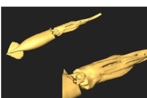
software could use this information to construct the three dimensional surface as given in Figure 5. Once the segmentation process was completed, the selected regions at each layer were interpolated to construct the three dimensional surface model in .stl format as shown in Figure 5(a). This surface model, expressed by small triangles, was then processed (Cignoni et al. (2008)) using Meshlab Software (v1.3.1 Visual Computing Lab) to repair common defects such as coincident points and voids. Finally, surface mesh quality was improved with a quadratic edge collapse decimation algorithm in the software and preprocessing of the three-dimensional squid surface was completed as shown in Figure 5(b). The finished squid surface was imported to the Rhinoceros v4.0 Software (Robert McNeal & Associates, 2008) to convert the .stl surface geometry into a .stp format solid model as shown in Figure 6, needed for finite volume analysis.
Fig. 5. Surface model after segmentation (top) surface model after defect cleaning and
smoothing (bottom).
Fig. 6. Finished squid model in .stp file format.
2.2 . Experimental Apparatus
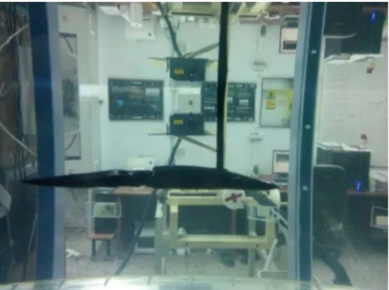
The three-dimensional squid model obtained from CT images was printed using a 3D printer (ZORTRAX M200, Zortrax S.A., Poland). Then, the manufactured squid model was used for digital particle image velocimetry (DPIV) experiments. The experiments were performed in a close-circuit water channel as shown in Figure 7. The water channel has a 8,000 mm × 1,000 mm × 750 mm test section with a maximum speed of 0.5 m/s and free stream turbulence intensity less than 1.5%. The test section of the water channel was made of transparent plexiglass with a thickness of 15 mm mounted on a steel frame. Straws placed into a wire mesh box were used as a flow straightener. The flow straightener was located prior to the contraction with ratio of 2:1.
The water was driven by a 15 kW centrifugal pump. The rotation speed of the pump can be controlled by a variable frequency drive controller unit. The water level was maintained at 450 mm during the experiments. The velocity measurements were carried out at water temperature of 20 ± 0.5ºC and ambient pressure of 100 ± 0.5kPa.
Fig. 7. Close-circuit water channel and printed squid model.
The two-dimensional digital particle image velocimetry (DPIV) system was used to measure the whole velocity field in the measurement plane. The complete DPIV system consists of a CCD (Charge coupled device) camera, a Nd:YAG laser system, laser sheet optics, a timer box, seeding (tracer) particles and a software. The measurement plane was illuminated by a thin laser light sheet that is 2 mm thick. The illumination was provided by a double-pulsed Nd:YAG laser with a repetition rate of 15 Hz and a typical energy of 2 × 120 mJ/pulse at a wavelength of 532 nm (New Wave Research, Solo 120XT) as shown in Figure 8.
A CCD camera with a spatial resolution of 1,600 × 1,200 pixels (Dantec Dynamics, FlowSense 2M) equipped with a lens that has a focal length of 60 mm (Nikon, AF Micro-Nikkor 60 mm f/2.8D) was used to record the movement of seeding particles as shown in Figure 9. The lens had a magnification factor M = 12.73. The CCD camera had a maximum operation frequency of 15 Hz in double-frame mode. The camera was synchronized with the pulsed laser, therefore, both the laser system and camera were operated at 15 Hz in the velocity measurements. A total of 1,000 image pairs were recorded in one set in order to compute further statistics. The flow medium was seeded by naturally buoyant silver-coated hollow glass spheres (S-HGS) with a mean diameter of 15 - 20 µm. The sketch of the experimental
(a)
apparatus is shown in Figure 10 to explicitly illustrate the location of the test model and direction of the fluid flow.
Fig. 8. 2 × 120 mJ/pulse at a wavelength of 532 nm laser seeing printed squid model in the
horizontal plane.
Fig. 9. CCD camera with 1600 x 1200 pixels spatial resolution seeing the printed squid
model from the bottom.
Fig. 10. Schematic view of the experimental set-up.
Calibration of PIV measurements were performed by placing a ruler onto the measurement plane at a certain distance from the CCD camera. Two different points on the ruler were selected with corresponding length scale using Dynamic Studio v3.2 software. This value was later used as a calibration constant between pixel in the image and real distance in the experiment. The freestream velocity of water channel was changed by a variable frequency drive
controller unit and velocity calibrations of the water channel were performed for various frequencies via PIV prior to starting experiments.
The position of the illuminating laser sheet remained fixed while the location of the camera varied to capture the three different flow domains in the measurement plane (Figure 11). The first field of view (FOV1) was selected to determine the freestream flow velocity and velocity distribution around the fore part of the test model. The FOV2 and FOV3 were selected to understand the effects of the fluid on the mid-part and aft part of the test model, respectively. The field of view was about 150.7 mm × 113 mm for FOV 1, 2 and 3. Dynamic Studio v3.2 software package was used for extracting the statistical data. After the image acquisition process, all image pairs were subdivided into interrogation windows (32 × 32 pixels) with overlaps of 50% in both horizontal and the vertical direction. Thus, the effective grid size was 3.01 × 3.01 mm2 for the plan-view measurements (Figure 11). The image from the first and the second pulse of the laser light-sheet were correlated by using an adaptive correlation technique to determine the average displacement vectors for each of these interrogation windows. Average displacement vectors were then converted into raw velocity vectors by dividing them with the known time between the image pairs (Dantec Dynamics). Totally 7,326 (99 × 74) velocity vectors were acquired at each instantaneous velocity field. Spurious (bad) vectors were estimated to be less than 3%. They were detected by applying the local-median filter technique and were replaced by interpolated vectors that were calculated by bilinear least-square fit technique between neighboring vectors.
Fig. 11. The various fields-of-view of the PIV images in the x-y plane (top view).
2.3
Computational Model Geometry,
Boundary Conditions and Meshing
The computational domain and boundary conditions for the numerical model are shown in Figure 12. The squid’s body length (L) and maximum body diameter were (D) measured to be 30 cm and 4.1 cm, respectively. The fineness ratio of a squid was defined as the ratio of body length (L) to maximum body diameter (D) and fineness ratio (L/D) was calculated to be 7.56 for the numerical model. The size of computational domain was chosen to be 9L in length, 6L in height and 6L in width after domain convergence tests were performed. The squid was positioned 3L distance from upstream and 5L distance from downstream. Left and right faces of the computational volume were defined as a velocity inlet and pressure outlet with zero gauge pressure
boundary conditions. The outer surface of the squid was set to a wall while upper and lower faces were identified as a slip wall boundary condition. When inlet boundary conditions were considered, turbulence intensity and viscosity ratio were utilized and specifically, turbulent intensity value of 1% and viscosity ratio of 10 were employed to the numerical model. The Reynolds number was defined as:
=
(1)In Eq. (1) ρ was density of fluid, U was the free stream velocity, L was the characteristic length (i.e., squid body length) and μ was dynamic viscosity of fluid. In the present work, three and six different swimming velocities were used in the experimental and numerical part of the study, respectively. ANSYS Fluent 12.1 computational fluid dynamics software was employed for the numerical model. While pressure-based coupled algorithm with SIMPLE scheme was utilized for the solution domain, type of discretization used for the advective terms of the transport equations were defined to be second order upwind schemes. Criteria of convergence was set to 10-6 for the governing equations. Total of 5 to 28 million tetrahedral and quadrilateral mesh elements were applied with high mesh density near the squid body as shown in Figure 13. Average aspect ratio was around 20 and these higher aspect ratio elements were mostly aligned with the freestream velocity. Average and maximum skewness ratios were nearly 0.3 and 0.55, respectively. Besides, the non-dimensional wall-distance parameter for the first cells was attended for shear stress transport (SST) k-ω model and the condition of <1 value for nodes nearest the wall was satisfied.
Fig. 12. Computational domain and boundary conditions of the numerical model.
Fig. 13. Tetrahedral and quadrilateral mesh elements in the solution domain.
The first layer thickness defined as:
=
,
(2)In Eq. (2) y could be estimated with Eq. (3) based on a flat plate theory.
= ×
× √80 ×
⁄(3)
The first layer thickness was selected to be 0.002 mm for turbulence flow simulations while ten boundary layers were chosen for meshes at the squid’s body wall by using an expansion factor of 1.3. Results of were obtained to be 0.95 at the maximum swimming velocity.
2.4 . Governing Equations
The Reynolds-averaged Navier-Stokes (RANS) equations and shear stress transport (SST) k-ω models were employed to the three-dimensional squid body model under the water. SST k-ω was used for CFD simulations because in this turbulence model, flow in the boundary layer (i.e., near the wall) was solved with k-ω model while flow outside the boundary layer (i.e., away from the wall) was governed by k-ε model. SST k-ω model known as a hybrid two equation model utilizes both k-ε and k-ω turbulent models for boundary layer and main flows, respectively. Besides, this model was verified to be suitable for high-Reynolds-number flows with separation (Menter (1994), Moshfeghi et al. (2012), Shereena et al. (2013), Vasudev et al. (2014), Rattanasiri et al. (2015), Tabatabaei et al. (2015), Malazi and Olcay (2016)).
The Reynolds-averaged Navier-Stokes (RANS) in indicial notation is defined as:
+
(
) = 0
(4)( )
+
= −
+
+
−
+
(−
, ,)
(5)where − , , is Reynolds stresses.
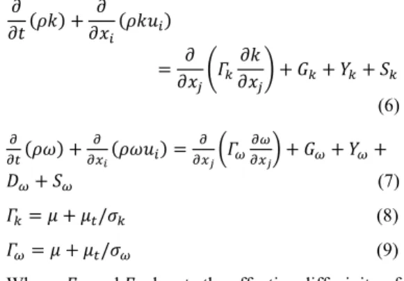
The Shear-Stress Transport (SST) k-ω model in indicial notation is given as Eq. (6) and Eq. (7)
( ) + ( ) = + + + (6) ( ) + ( ) = + + + + (7) = + / (8) = + / (9)
Where, , and denote the effective diffusivity of k and ω, respectively while and represent the generation of turbulence kinetic energy and ω, respectively. and denote the dissipation of k and ω, respectively due to turbulence and represents the cross-diffusion term while and are user-defined source terms (See ANSYS Inc., for
Fig. 14. Comparison of DPIV and CFD velocity contour plots for inlet velocities of 78.6 mm/s (upper), 115.7 mm/s (middle) and 160.1 mm/s (lower).
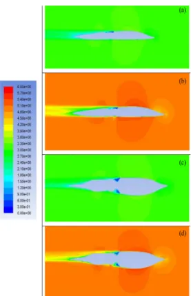
Fig. 15. Velocity contour plot for Reynolds numbers of 949900 (a, c) and 1510400 (b, d). The
front and top views of the squid model were illustrated in (a, b) and (c, d), respectively.
other details). The SST k-ω turbulence model was used for model that velocities are at turbulent regions and also the value of y was attended for SST k-ω turbulence model at all numerical calculations.
3. R
ESULTSA
NDD
ISCUSSION3.1
Velocity Contour Plots of DPIV
Measurements and Numerical Models
DPIV measurements were performed for the printed three-dimensional squid model at three different Reynolds numbers. The highest Reynolds number for the squid was 47210 because the close-circuit water channel could provide 160.1 mm/s as the highest water velocity throughout the channel. Meanwhile, the three-dimensional numerical model simulations were executed to provide comparison between experimental and numerical velocity contours around the three-dimensional squid models. As revealed in Figure 14, the velocity contours in the numerical models agree well with the velocities obtained from DPIV measurements for Reynolds numbers of 23177, 34117, 47210.A squid having a flexible mantle wall can swim either slow or fast modes under water. The movement rate of mantle wall generally determines the squid’s swimming mode. Since the goal of this study is to understand the squid’s flow characteristics, Figure 15 is given here to show how the velocity around the three-dimensional squid
model varies for Reynolds numbers of 949900 and 1510400. It was noted that the velocity vectors followed the squid’s outer surface for Reynolds number of 949900 (Fig. 15(a) and 15(c)) except the squid head region. Flow separation could be observed near the head region because the velocity contour values fell nearly to zero at that location. When Reynolds number becomes 1510400, flow separation could be observed in the front and top views of the model (Fig. 15(b) and 15(d)) specifically for the region starting from head to the end of the tentacles yielding larger drag force exposure. In addition to velocity contour plots, pressure contour plots are shown in Figure 16. It was realized that the numerical model with Reynolds number of 1510400 shows lower pressure regions around the head region implying flow separation.
Fig. 16. Pressure contour plot for Reynolds numbers of 949900 (a, c) and 1510400 (b, d). The
front and top views of the squid model were illustrated in (a, b) and (c, d), respectively.
3.2 Hydrodynamic Force Study
The drag force appears on a body whenever the body moves in a fluid. Especially, if the fluid is water being nearly 1000 times heavier than air, the body can suffer from a large drag force during its underwater travel. In this part of the study, drag force FDrag acting on a swimming squid was calculated
based on Eq. (10)
= _ + _ . (10) Here, pressure drag (FD_pressure) was associated with
the pressure variation, namely normal stress, along the squid body while viscous drag (FD_viscous) was
related to the shear stress developing at the outer surface of the squid body. The drag force was calculated for the numerical squid model at various swimming velocities and plotted in Figure 17. It was
noted that the drag force increased with increasing squid swimming velocity and reached its peak value at Re = 1510400. Figure 17 also revealed that viscous drag was more dominant than the pressure drag because a swimming squid exhibited a streamlined body behavior. In addition to drag force calculation, the drag coefficient was calculated using Eq. (11)
=
.
(11)
Fig. 17. Variation of total, pressure and viscous drag along with Reynolds number.
Here, CD is the drag coefficient, FDrag is the total drag
acting on the body when the body moves in the fluid, ρ is the density of the fluid, U is the velocity of the fluid relative to the body, A is the characteristic area of the body, more specifically the squid’s surface area.
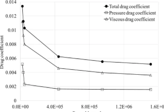
As revealed from Figure 18, the drag coefficient decreased with an increasing squid swimming velocity. Moreover, the total drag coefficient reached nearly 0.005 agreeing with Malazi et al. (2015) when Reynolds number was 1510400. Similarly, the contribution of the viscous drag coefficient to the total drag coefficient was more than the contribution of the pressure drag coefficient. This implies that the streamlined body of a squid would mainly be exposed to the drag associated with the viscous effects.
Fig. 18. Variation of total, pressure and viscous drag coefficient along with Reynolds number.
3.3
Determination of Jet Velocities
Based on Nozzle Diameter
A squid known to be the excellent swimmer of
0 0.2 0.4 0.6 0.8 1 1.2 1.4 1.6 1.8
0.0E+00 4.0E+05 8.0E+05 1.2E+06 1.6E+06
D rag fo rce (N ) Reynolds number Total drag Pressure drag Viscous drag 0 0.002 0.004 0.006 0.008 0.01 0.012 0.014
0.0E+00 4.0E+05 8.0E+05 1.2E+06 1.6E+06
D rag co ef fi ci en t Reynolds number
Total drag coefficient Pressure drag coefficient Viscous drag coefficient
marine life appreciates the variety of muscular structure surrounding her. For example, a mantle wall of a squid formed by bundles of circular and radial muscles (Gosline and Demont 1985) covers the mantle cavity and a squid generally uses mantle cavity to store the water inside so that it can be ejected for rapid acceleration. Similar to the mantle wall, a nozzle of a squid is made of a series of circular muscles and a squid can easily control the diameter of her nozzle to adjust the velocity of water jet. In this part of the study, the effect of nozzle diameter on squid’s swimming speed was investigated. A control volume analysis of an unsteady two-dimensional axisymmetric squid model (Malazi and Olcay 2016) was implemented for the steady three-dimensional squid model to determine the relationship between the nozzle diameter and required jet velocity for the desired cruise speed of a squid. In the present work, the nozzle diameter of a longfin inshore squid was measured to be 1 cm. Therefore, three different nozzle diameters (0.005, 0.01 and 0.02 m) were chosen to calculate the required jet velocity using Eq. (12)
= ( − ) (12) Here, ρ is density of the fluid, A is cross-sectional area of the jet and Ujet and Uvehicle are the jet and
vehicle's velocity (squid’s swimming velocity in the present study), respectively. Thrust force (FT) is described as the force being equal to the drag force a squid experiences during her steady swimming under water. Figure 19 illustrates the required jet velocity of a squid for six different squid cruise velocity. It was noted that whereas nozzle diameter was decreased from 0.02 m to 0.005 m, a squid had to provide nearly two times larger jet velocity thru her nozzle to reach the same cruise velocity. This implied that a squid likely expands her nozzle diameter during jet ejection; therefore, the squid would require less jet velocity.
Fig. 19. Relationship between squid velocity and jet velocity for three different nozzle diameters.
3.4 Jet Propulsive Efficiency Study
The performance of an underwater vehicle is generally determined based on the efficiency of the driving system of that vehicle. Therefore, jet propulsive efficiency has become a vitally important parameter in the analysis of an underwater vehicle locomotion. The jet propulsive efficiency could be
defined with Eq. (13) (Moslemi and Krueger (2010)) = 2/(1 + ⁄ ) (13) Here, Uvehicle is the underwater vehicle's velocity
(squid’s swimming velocity in the present study) and Ujet is jet propulsive velocity. In this work, the jet
propulsive efficiency was calculated for the six different squid swimming velocities when nozzle diameters varied between 0.005 and 0.02 m as shown in Figure 20. It was understood that the jet propulsive efficiency increased with increasing squid velocities and it reached peak value around 90% for nozzle diameter of 0.02 m.
Fig. 20. Variation of propulsive efficiency with Reynolds number for three different nozzle
diameters.
4. C
ONCLUSIONIn this study, fluid flow characteristics of an inshore longfin squid were investigated for six different swimming velocities. The CT images provided virtually all the details of the squid’s outer shape and a three-dimensional squid shape was printed and placed into a close-circuit water channel for DPIV measurements. The results of the numerical three-dimensional model agreed well with the results of DPIV measurements for the three different squid velocities. Then, three additional swimming velocities were identified for the squid and fluid flow around the squid model was examined. Drag force and drag coefficient calculations were performed and it was found that viscous drag contributed to total drag more than pressure drag because of the streamlined shape of the swimming squid. Furthermore, the relation between required jet and squid cruise velocities was determined from the control volume analysis for the different squid nozzle diameters.
The propulsion efficiency of the squid model exhibited sharp increase when the flow characteristics varied from laminar to turbulent regime. This indicated that squid shape underwater vehicles could benefit more from propulsion efficiency if they stay in the turbulent flow regime. Besides, once the flow is in the turbulent regime, propulsion efficiency nearly remains constant. It was also reported that when a squid used a larger nozzle
0 2 4 6 8 10 12 14 0 1.5 3 4.5 6 Je t ve loc ity ( m /s ) Squid velocity (m/s) Nozzle diameter = 0.005 m Nozzle diameter = 0.01 m Nozzle diameter = 0.02 m 0.4 0.5 0.6 0.7 0.8 0.9 1
0.0E+00 4.0E+05 8.0E+05 1.2E+06 1.6E+06
P rop ul si on e ff ic ie nc y Reynolds number Nozzle diameter = 0.005m Nozzle diameter = 0.01m Nozzle diameter = 0.02m
diameter to move under water, she would need a lower jet velocity requirement. This actually implied that a larger nozzle diameter provided higher propulsive efficiency based on the relation between the jet and squid’s cruise velocities.
A
CKNOWLEDGEMENTSThis work has been supported by TUBITAK (The Scientific and Technological Research Council of Turkey) under 3501 Program, Project #: 111M598.
R
EFERENCESAnderson, E. J. and M. A. Grosenbaugh (2005). Jet flow in steadily swimming adult squid. J. Exp. Biol. 208, 1125–46.
Bartol, I. K., P. S. Krueger, W. J. Stewart and J. T. Thompson (2009). Hydrodynamics of pulsed jetting in juvenile and adult brief squid Lolliguncula brevis: evidence of multiple jet ‘modes’ and their implications for propulsive efficiency. The Journal of Experimental Biology 212, 1889-1903.
Bilo, D. and W. Nachtigall (1980). A simple method to determine drag coefficients in aquatic animals. J. Exp. Biol. 87, 357–359.
Cignoni, P., M. Corsini, G. Ranzuglia (2008). Meshlab: An open-source 3D mesh processing system. Ercim news 73, 45-46,
Evans, J. and M. Nahon (2004). Dynamics modeling and performance evaluation of an autonomous underwater vehicle. Ocean Eng. 31, 1835–1858. Gosline, J. M. and M. E. DeMont (1985). Jet-propelled Swimming in Squids. Sci. Amer. 256, 96-103.
Karim, M., M. Rahman and A. Alim (2008). Numerical computation of viscous drag for axisymmetric underwater vehicles. Jurnal Mekanikal 26, 9–21.
Malazi T. M. and A. B. Olcay (2016). Investigation of a longfin inshore squid's swimming characteristics and an underwater locomotion. Applied Ocean Research 55, 76-88.
Mansoorzadeh, S. and E. Javanmard (2014). An investigation of free surface effects on drag and lift coefficients of an autonomous under water vehicle (AUV) using computational and experimental fluid dynamics methods. J. Fluids Struct. 51, 161–171.
Menter F. R. (1994). Two-equation Eddy-viscosity turbulence models for engineering applications. AIAA J. 32(8), 1598-605.
Moshfeghi, M., Y. J. Song and Y. H. Xie (2012). Effects of near-wall grid spacing on SST-K-ω model using NREL Phase VI horizontal axis wind turbine. Journal of Wind Engineering and Industrial Aerodynamics 94-105.
Moslemi, A. A. and P. S. Krueger (2010). Propulsive efficiency of a biomorphic pulsed-jet underwater vehicle. Bioinsp. Biomim. 5.
Nematollahia, A., A. Dadvandb and M. Dawoodian (2015). An axisymmetric underwater vehicle-free surface interaction: A numerical study. Ocean Engineering 96, 205-214.
Ozgoren, M., A. Okbaz, S. Dogan, B. Sahin and H. Akilli (2013). Investigation of flow characteristics around a sphere placed in a boundary layer over a flat plate. Experimental Thermal and Fluid Science 44, 62–74.
Ozgoren, M., E. Pinar, B. Sahin and H. Akilli (2011). Comparison of flow structures in the downstream region of a cylinder and sphere. International Journal of Heat and Fluid Flow 32(6), 1138– 1146.
Qian, P., H. Yi and Y. Li (2015). Numerical and experimental studies on hydrodynamic performance of a small-waterplane-area-twin-hull (SWATH) vehicle with inclined struts. Ocean Engineering 96, 181–191.
Randeni, S. A. T., Z. Q. Leonga, D. Ranmuthugalaa, A. L. Forresta and J. Duffyaa (2015). Numerical investigation of the hydrodynamic interaction betweentwo underwater bodies in relative motion. Applied Ocean Research 51, 14–24. Rattanasiri P., P. A. Wilson and A. B. Phillips
(2015). Numerical investigation of a pair of self-propelled AUVs operating in tandem. Ocean Engineering 100, 126–137.
Shereena, S. G., S. Vengadesan, V. G. Idichandy and S. K. Bhattacharyya (2013). CFD study of drag reduction in axisymmetric underwater vehicles using air jets. Eng. Appl. Comput. Fluid Mech. 7, 193–209.
Stewart, W. J., L. K. Bartol and P. S. Krueger (2010). Hydrodynamic fin function of briet squid, Lolliguncula brevis. The Journal of Experimental of Biology 213, 2009-2024.
Tabatabaei, M. M., A. Okbaz and A. B. Olcay (2015). Numerical investigation of a longfin inshore squid's flow characteristics. Ocean Engineering 108, 462-470.
Vasudev K. L., R. Sharma and S. K. Bhattacharyya (2014). A multi-objective optimizationdesign framework integrated with CFD for the design of AUVs. Methods in Oceanography 10, 138–65. Yalcinkaya, B. H., S. Erikli, B. A. Ozilgen, A. B.
Olcay, E. Sorguven and M. Ozilgen (2016). Thermodynamic analysis of the squid mantle muscles and giant axon during slow swimming and jet escape propulsion. Energy 102, 537-549. Zhou, H., T. Hu, K. H. Low, L. Shen, Z. Ma, M.
Wang and H. Xu (2015). Bio-inspired Flow Sensing and Prediction for Fish-like Undulating Locomotion: A CFD-aided Approach. Journal of Bionic Engineering 12, 406–417.