ANALYSIS OF CYLINDRICAL REFLECTOR
ANTENNAS IN THE PRESENCE OF CIRCULAR
RADOMES BY COMPLEX SOURCE-DUAL SERIES
APPROACH
A DISSERTATION
SUBMITTED TO THE DEPARTMENT OF ELECTRICAL AND ELECTRONICS ENGINEERING
AND THE INSTITUTE OF ENGINEERING AND SCIENCES OF BILKENT UNIVERSITY
IN PARTIAL FULFILLMENT OF THE REQUIREMENTS FOR THE DEGREE OF
DOCTOR OF PHILOSOPHY
By
Tañer Oguzer
November 1996
T oner O ^uaer tarafittdan ba¿islannu§lir.к
I certify that I have read this thesis and that in iny opinion it is fully adequate, in scope and in quality, as a dissertation for the degree of Doctor of Philosophy.
3 ^ ·
Prof. Dr. Ayhan Altmtaş(Supervisorj
I certify that I have read this thesis and that in iny opinion it is fully adequate, in scope and in quality, as a dissertation for the degree of Doctor of Philosophy.
Assoc. Prof. Dr. Ill adi Aksun. I r lt
I certify that I have read this thesis and that in my opinion it is fully adequate, in scope and in quality, as a dissertation for the degree of Doctor of Philosophy.
r. Vladimir Yurchenko
I certify that I have read this thesis and that in my opinion it is fully adequate, in scope and in quality, as a dissertation for the degree of Doctor of Philosophy.
r h - f r / ^
Assoc. Pro f. Dr.Viğurhan Mugan
I certify that I have read this thesis and that in my opinion it is fully adequate, in scope and in quality, as a dissertation for the degree of Doctor of Philosophy.
Assoc. Prof. Dr. Giilbin Dural
Approved for the Institute of Engineering and Sciences:
Prof. Dr. lV^eJ>met Baray
ABSTRACT
ANALYSIS OF CYLINDRICAL REFLECTOR ANTENNAS
IN THE PRESENCE OF CIRCULAR RADOMES BY
COMPLEX SOURCE-DUAL SERIES APPROACH
Taner Oğıızer
Pli. D. in Electrical and Electronics Engineering
Supervisor: Prof. Dr. Ayhan Altıntaş
November 1996
The radiation from cylindrical reflector antennas is analyzed in an accurate manner for both H and E polarization cases. The problem is first formulated in terms of the dual series equations and then it is regularized by the Riemann- Hilbert Problem techiiicpie. The resulting matrix equation is solved numerically with a guaranteed accuracy, and remarkably little CPU time is needed. The feed directivity is included in the analysis by the complex source point method. Various characteristic patterns are obtained for the front and offset-fed reflector antenna geometries with this analysis and some comparisons are made with the high frequency techniques. The directivity and radiated power properties are also studied. Furthermore, the results are also compared by the .Method Of Moments and Physical Optics solutions. Then the case of circular radorne enclosing the reflector is considered. Radomes concentric with the reflector are examined first, followed by the non-concentric radomes.
Keywords: Cylindrical reflector antennas. Radiation, Radome, Dual series ecpiations.
ÖZET
d a ir e s e l
RADOMLU SILINDIRIK YANSITICI
ANTENLERİN KARMAŞIK KAYNAK-İKİLİ SERİLER
YAKLAŞIMIYLA ANALİZİ
Taner Oğıızer
Elektrik ve Elektronik Mühendisliği Bölümü Doktora
Tez Yöneticisi: Prof. Dr. Ayhan Altıntaş
Kasım 1996
Siliııclirik yansıtıcı antenlerden radyasyon her iki II and E polarizasyonlar için hassas bir biçimde analiz edildi. Problem önce ikili seri denklemleriyle formüle edildi ve sonra Riemann-Hilbert tekniğiyle düzenlileştirildi. Sonuçtaki ma tris denklemi nümerik olarak garantili hassasiyetle çözüldü. Kaynak kazancı analize karmaşık kaynak noktası yöntemiyle dahil edildi. Pek çok karakter istik örnekler önden ve kaydırılmış beslemeli yansıtıcı anten geometrileri için aynı yöntemle elde edildi ve yüksek frekans teknikleriyle bazı karşılaştırmalar yapıldı. Kazanç ve radyasyon gücü özellikleri üzerinde de çalışıldı. .Ayrıca, sonuçlar moment yöntemi ve fiziksel optik çözümleriylede karşılaştırıldı. Daha sonra \ ansiticiyi çevreleyen dairesel radonı durumu düşünüldü. A^ansıtıcı ile or tak merkezli radomlar önce sınandı ardından da ortak merkezli olmayan radom- 1ar incelendi.
.Anahtar sözcükler: Silindirik yansıtıcı antenler, radya.syon, radorn, ikili seri denklemleri.
ACKNOWLEDGMENT
I would like to express my deep gratitude to Prof. Dr. .A,yhan .Altinta.^ and Dr. .Alexander I. Nosich for their suggestions, help and invaluable guidance during the development of this thesis.
C on ten ts
1 INTRODUCTION 1
2 COMPLEX SOURCE POINT METHOD 4
2.1 Form ulation... 4
2.2 Comparison of the complex source point and the typical aperture beam p a tte rn s ... 7
3 MATHEMATICAL BACKGROUND FOR RHP METHOD 9 3.1 Introduction... 9
3.2 Riernann-Hilbert Problem in the Complex Variable Theory . . . 10
3.3 Solution of the Riemanri-Hilbert P ro b lem ... 12
3.4 Solution of Canonical Dual Series E cjuations... 13
4 REFLECTOR IN FREE SPACE 16 4.1 Formulation of the p r o b le m ... 16
4.2 Approximation of a parabolic reflector by a circular o n e ... 19
4.3 Dual series eciuations for E and H polarization cases... 20
4.4 RHP solution and symmetry sp littin g ... 22
4.5 Physical Optics s o lu tio n ... 24
4.6 Method of Moments solution... 26
CONTENTS vii
4.7 Far field characteristics... 26
5 REFLECTOR INSIDE A RADOME 28
5.1 Radiation in the presence of a circular ra d o in e ... 28
5.2 Concentric radome case 29
5.3 Nonconcentric radome c a s e ... 32
6 NUMERICAL RESULTS 36
6.1 Reflector in free space 37
6.2 Directivity and radiated pow er... 49 6.3 Reflector inside a radoine... 50
7 CONCLUSIONS 66
A Explicit expressions for some functions appearing in Chapter
L ist o f F igures
2.1 Geometry of a coinplex-source-point model. .5
2.2 Comparison of the complex source point and the aperture beam far-held pattern of ecpiation (2.17). ka=4 for the aperture and kb=3 for the complex source. Solid line represents the complex source point pattern and the dashed line represents the aperture beam pattern of ecjuation (2.17)... 8
3.1 Simple closed curve on the complex p lan e ... 11
4.1 Circular offset reflector antenna geometry... 17 4.2 Equal-value curves of the electrical error( A/A) and the reflector
size(/A/A) as a function of ka and Oap. Solid curves represents constant reflector size and dashed curve represents constant elec
trical error. 21
4.3 Front fed symmetrical reflector antenna geometry 2.5
5.1 Circular reflector in the presence of concentric radom e... 29 5.2 Circular reflector in the presence of nonconcentric radome 33
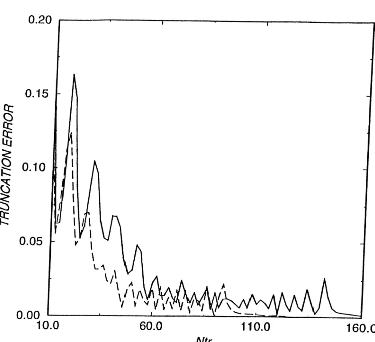
6.1 Truncation error dependence on the matrix order, for two sample geometries: ka=100(dashed curve) and ka=150 (solid curve).
e,=0, 0ap=W, kb=9... 38
6.2 CPU times for both polarizations... 39
LIST OF FIGURES IX
6.3 Comparison of E-Polarization radiation pattern of a parabolic reflector [2] (F/D=0.96, D=10A) with a circular one (ka=120..57, ^aP=15"). Feed directivity parameter. kb=9.06 corresponds to
a —10.09 c/jP edge illumination. 40
6.4 Comparison of E and H polarization radiation patterns for a front-fed symmetrical circular reflector of ka= 120.57. O^p = b5° where D=10A and 9o = = 0°. Feed parameters are A7’^=60.28,
kb=9.06( —l0.09clB edge illumination). 41
6.5 Comparison of E and H polarization radiation patterns for a off set circular reflector of ka=120.57. 0.^ = 15.9P, Oo = '22'^ where
D = 9.77A. Feed parameters are A-r, = 60.28, feed beaming
angle /? = 39° and kb=11.05 corresponds to a -9.7S dB and
— \9.lAdB edge illuminations for lower and upper edges. 42 6.6 Comparison of the physical optics radiation patterns with the
present solution for a front-fed symmetrical circular reflector of ka=120.57, Oap = 15°(D=10A). Feed parameters are
kb=9.06( —10.09f//? edge illumination): E-Polarization case. . . 43 6.7 Comparison of the physical optics radiation patterns with the
present solution for the same geometry as in Figure 6.6: H- Polarization case... 44 6.8 Comparison of method of moments solution with the method of
regularization result for E polarization case. Front-fed symmet rical circular reflector of ka=62.S, OaP — 29.7A'(D = lOA). Feed parameters are kro=31.4 and kb=2.6 (-9 clB edge illumination). 45 6.9 Comparison of method of moments solution with the method
of regularization result for H polarization case for the previous geom etry... 16 6.10 Radiation patterns of large circular oiset reflector for F/ Dp —
0.3, h/D=0.125 and D = 50A where Oap = 25.56° and 0.^ = 30.87°. Feed taper is defined with the source directivity param eter kb=5.46 corresponding to —10 dB for a half angle Us of 37.895°... 47
LIST OF FIGURES
6.11 Radiation pattern comparison of PO and RHP for the beam aiming angle of 48.475'’ with the source directivity parameter kb=5.46 for a —10dB half angle edge illumination. 48 6.12 Effect of the different edge taperings for E-Polarization ca.se for
a front-fed symmetrical reflector with ka=62.8, 0,jp = 29.74° (D=9.92A). Feed directivity parameters, kb=.3.5 and kb=5 cor respond to —1.3.02f/i? and —18.21 di? edge illuminations... 51 6.13 Effect of the different edge taperings for H-Polarization ca.se for
a front-fed symmetrical reflector with ka=62.8, = 29.74° (D=9.92A). Feed directivity parameters, kb=3.5 and kb=5 cor respond to —l3.0'2dB and —18.21 edge illuminations... 52 6.14 Effect of the different aperture dimensions for E-Polarization
case for a front-fed symmetrical reflector of the constant angu lar halfwidth 6ap = 29.74°. Feed directivity parameter kb=5 provides —18.21 dB edge illumination... 53 6.15 Effect of the different aperture dimensions for H-Polarization
case for a front-fed symmetrical reflector of the constant angu lar halfwidth O^p = 29.74°. Feed directivity parameter kb=5 provides —18.21 edge illumination... 54 6.16 Total radiated power variation with increasing aperture dimen
sion for a front-fed symmetrical reflector of Oap = 15° and f/D=0.96. Feed directivity parameter kb=1.5 corresponds to — 1.65 dB edge illumination... 55 6.17 Directivity variation with increasing aperture dimension for a
front-fed symmetrical circular reflector of Oap — 15° and f/D=0.96. Feed directivity parameter k b = l.5 corresponds to —l.OodB edge illumination... 56 6.18 Total radiated power variation with increasing feed directivity
parameter kb, for Oap = 15° and ka=50 (D=3.9A). 57 6.19 Directivity variation with increasing feed directivity parameter
kb, for Oap = 30° and ka=62.8 (D=10A). 58
6.20 Variation of the directive gain with the beam aiming angle for the circular offset reflector of F/Dp — 0.3, h/D=0.125 and D —
LIST OF FIGURES XI
6.21 Variation of the spilloverlobe levels in dB with the beam aiming angle for the circular offset reflector of F/Dp = 0.3, h/D=0.12.5 and D = 50A where = 25.56° and 0^ = 30.87°... 60 6.22 The radome effect on the radiation pattern for E-Polarization
case. The radome geometry is defined as ka = 62.8, kc = 78.5 and t = 0.5A¿. The permitivity of dielectric shell is 2. Feed directivity parameter kb = 2.6 corresponds to a —9.92 dB edge
illumination. 61
6.23 The radome effect on the radiation pattern for H-Polarization case. The radome geometry is defined as ka = 62.8, kc — 78.5 and t = 0.5Aj. The permitivity of dielectric shell is 2. Feed directivity parameter kb — 2.6 corresponds to a —9.92 dB edge
illumination. 62
6.24 The radome effect on the radiation pattern for E-Polarization case. The radome geometry is defined as ka = 62.8, kc = 78.5 and t = 0.5Ad. The permitivity of dielectric shell is 2. Feed directivity parameter kb = 5 corresponds to a —18.21 dB edge illumination... 63 6.25 The radome effect on the radiation pattern for H-Polarization
case. The radome geometry is defined as ka = 62.8, kc = 78.5 and t = 0.5A¿. The permitivity of dielectric shell is 2. Feed directivity parameter kb = 5 corresponds to a —18.21 dB edge illumination... 64 6.26 The radome effect on the radiation pattern for H-Polarization
case. The radome is nonconcentrically located. The radome geometry is defined as ka = 31.4, kc = 27.3, kL = 27.3 and thickness of the radome is i = 0.5Aj (dashed curve) and i = 0.4Ad (dotted curve). The permitivity of dielectric shell is 2. Solid curve represents the reflector in free space. Feed directivity parameter kb = 2.6 corresponds to a —9dB edge illumination. . 65
C h apter 1
IN T R O D U C T IO N
High frequency techniques such as the Aperture Integration (AI) and the Ge ometrical Theory of Diffraction (GTD) are commonly employed for predicting the far-field radiation characteristics of electrically large reflector antennas. In the papers of Suedan and dull [1,2], it is demonstrated that the Complex Source Point (CSP) method can be successfully used in combination with AI or GTD to take account of source directivity in reflector antenna simulations, since the replacement of the real coordinate of a uniform source with the complex one generates a beam field in real space [3]. However, both AI and GTD have well-known internal shortcomings for reflector antenna problems. The former gives less accurate results off the main beam, and completely fails in shadow region. The latter, oppositely, is not applicable in the main beam direction. That is why, usually, one has to compose the results of two methods, without any clear rule of choosing the matching point. Although these high frequency techniques are applicable to many practical problems, the range of validity of the results, in terms of acceptable accuracy is unpredictable.
Provided that the reflector is not electrically large, more accurate results can be obtained by numerical techniciues, such as method of moments (MoM). Normally the matrix size involved in computations with this method is 10 to 30 times the parameter D/A, where D is the reflector dimension and A is the wavelength. If the entire-domain basis functions are used [4], the matrix size can be smaller but the matrix filling time increases impressively. In any ca.se, the accuracy and convergence properties are quite dependent of the implemen tation.
Therefore, there is still a need for a technique for the analysis and simu lation of the reflector antennas with any desired accuracy. We present such a technique for circular cylindrical reflectors in which the dual series formulation
CHAPTER 1. INTRODUCTION
is used in combination with the complex source point approach. The aim is to demonstrate the unique opportunities offered by using this combination.
In the core of the analysis, there is the idea of regularization, i.e., a partial inversion of original integral operator. In our treatment, the inverted part of the integral operator is its static part. First, we reduce the problem to dual series equations [5-8] for surface current expansion coefficients. Then, we extract certain canonical equations and solve them exactly using Riemann- liilbert Problem technique. The details of this approach, as it is used here, can be found in the references [5-8]. The resulting matrix equations enable one to conclude two facts of primary importance. First, the exact solution to the infinite matrix equation really exists, and second, it can be approximated with a desired accuracy (within digital precision) by .solving truncated equations of large enough order. Actually, in far field computations with the uniform accuracy of 0.1%, the needed matrix size is only ka plus 5 to 10 for a realistic circular front-fed reflector of radius a.
To use the dual series approach for the simulation of reflector antennas, one has to restrict the reflector geometry to a circular cross-section. Although actual reflectors are of parabolic shape, the aperture dimensions compared to focal distance are often rather small. This offers a way to approximate the parabola by a part of a circle with great accuracy, and thus to avoid the modification of the method.
To protect the reflector antenna system from the enviromental conditions, radomes are commonly used. The performance of the reflector antenna is changed by the presence of the radome, however almost distortionless trans mission is possible if the radome satisfies some electromagnetic requirements. The reflector antenna covered by a radome is analyzed by the method devel oped in this thesis. Normally, it is not easy to obtain the exact reference data for the given reflector and radome geometries by the other numerical methods like the method of moments. The present method gives, however, the exact solutions to the problems with any desired accuracy. By using the solutions, the far field radiation patterns as well as the directivity and the total radi ated power are evaluated for the different radome and reflector electrical and geometrical parameters.
The outline of the thesis is as follows. In Section 2 following the introduc tion, the complex source point method is described and compared with the typical aperture beam approach. In Section 3, a mathematical background for the Riemann-Hilbert Problem technique is discussed. In Section 4, this
CHAPTER 1. INTRODUCTION
technique is used to solve the problem of a 2D circular reflector in the free space for both E- and H-polarization cases. The given approach is compared with the conventional physical optics and method of moments solutions, and the formulas for various far-field characteristics are presented. The similar but more complicated problem of the reflector inside a concentric or nonconcentric 2D circular dielectric radome is considered in Section -5. The numerical results for all the problems are presented in Section 6, and the concluding remarks are summarized in the final Section.
The time dependence e is assumed and omitted throughout the further analysis.
C h apter 2
C O M P L E X SO U R C E P O IN T M E T H O D
2.1
F orm ulation
In a homogeneous unbounded medium, replacement of the line source posi tion from real to complex one, creates a beam field in two dimensions (2D). This implies that complex source point(CSP) substitution converts line source Green’s functions into field solutions for incident directive beams. Thus, with out further effort, the whole diffraction solutions yield the field response for beam excitation, provided there can be analytic continuation of the solutions from real space to complex space.
Figure 2.1 shows a 2-dimensional line source at {I'ofto) from the origin of coordinates. The fields are uniform in the z direction and represent an oiîuii- directional cylindrical wave. The field intensity at any observation point \\0 which is a solution of the wave equation may be written as
u = 7 i / ‘> k R » i (2 J)
where k = it;/c and is the Hankel function ol the first kind and R is the distance of the observation point from the source.
R = \/r'^ + r l ~ 2rro cos{0 - 6o). (2.2)
In the far field (r > > r^), R = r - r<,cos(^ - Oo) applies in the pha.se term and R ~ r in the amplitude term of (2.1) giving
CHAPTER 2. COMPLEX SOURCE POINT METHOD
Field Point
Figure 2.1: Geometry of a cornplex-.source-point model.
^ i k { r — r o c o s { 6 — 9 o ) )
u‘" ( r J ) = C ---^
where C is the complex constant.
0 < Or, < K (2.3)
By making the source coordinates {ro,9o) complex (/^.(9,,), one converts the omnidirectional wave into a directive beam uniform in the z direction. Here,
- K + ib (2.4)
and b are the complex source position, real source position and beam parameter vectors given in polar coordinates as ro=0'ofio)·, P?=(rs-<9,,) and 6=(b,/?), where b defines the sharpness of the beam and 3 defines its ori entation. All angles are measured from the x-axis. The \alues of and 0^ are [1,2]
r, = \ J r lT 2ivobcos{3 - Oo) — b'^ Rc{fs) > 0
^ r-oCOs(Oo) + ibcOs{3) ^
Og = arccos(--- )
T s
where 6 > 0 and 0 < /9 < 27t. Replacing Vo,0o by rg.Og gives
Jk(r-T^ cos(6-6s)) U \v,D) =
C-\/kr r » r.
Tg cos{0 - Og) = r, cos(^3) cos(t?) + rgsin(i?J sin(t?)
rgcos{0g) = rocos{0o) + ibcos{3)
(2.5) (2.6)
(2.7) (
2
.8
) (2.9)CHAPTER 2. COMPLEX SOURCE POIXT METHOD
rs S in (0 j,) = roSin(^c-) + > b s \ n { / 3 )
Using these in (2.8) yields
t's c o s { 6 — 6 s ) = Vo c o s { 0 — O . j ) + i b c o s ( 0 - 0 ) (2.10) (2.11) Substituting (2.11) in (2.7) we get ^ i k ( r - r o c o s { 6 — 6 r j ) ) u''\r,9) = C --- ^ ---^UcoMO-,3) y k r
(2.12)
By comparing equation (2.12) with (2.3) we find that (2.12) represents an omnidirectional cylindrical wave (first term) modulated by a beam pattern gfc6cos(i9-/5) Y^rith its maximum in the direction 0 = 0 and minimum in the direction 0 0 -\- K.
The incident field due to the line source of amplitude C at the complex position Cs is given by
■«‘'•(f) = C7/<‘) ( ^ |r - U ,|) . (2.13)
With the use of the addition theorem for the Haid<el functions, it can be written as
r C \ r , < f ) ^ C X : J„(AT,)//(‘)(^v)e‘'‘(·’''- '’)
r
> fs (2.14)For the reflector antenna geometries, an important parameter is the total radiated power P normalized to the radiated power Pq of the complex line
source in free space. Pq is easily found by integrating the squared absolute value of the function (2.13) over the circle of a large enough icvdius k-\r — ;^| > > 1, and is given by
- Vi)
(2.15)
Po = C^'^Io(2kb)
where r; is (^o)~* and Zq for E and H-polarization cases, respectively. Zq is the intrinsic impedance of free space and /q is the modified Bessel function of order 0.
2.2
C om parison o f th e co m p lex source point and th e
ty p ica l a p ertu re beam p a ttern s
CHAPTER 2. COMPLEX SOURCE POINT METHOD 7
We normalize the field of (2.12) to its peak value
■{d'"(r,/9)
^ g-A-6(l-cos(e-J))
(2.16) In the far zone, equation (2.1.3) behaves like equation (2.16). Therefore, at far zone, we use equation (2.11) as the comple.x source point field. Furthermore, complex source point field behaves iis a Gaussian beam in the paraxial region.
Typical aperture beam pattern is an inphase cosinusoidal distribution in an aperture of width 2a. Its normalized pattern is
«‘"■(r, 0) cos{ka sin(<? — /9))
u”‘(r,/9) 1 — (^ sin(61 —/9))·^’ and for ka=4, its half-power bearnwidth is 55.7°.
(2.17)
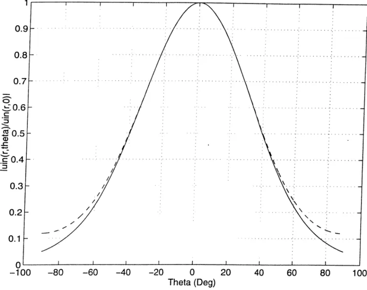
One can plot the beam patterns for the aperture of width 2a, as given in (2.17) with the pattern of the complex source given in (2.16) to get a com parison. For this purpose, the beamwidths of two patterns are equated using parameter ”a” for the aperture and ”b” for the complex source. Such a com parison is shown in Figure 2.2 . Obviously, complex source point method gives pattern for whole space although typical aperture beam patterns are only for a half space that field radiates. Therefore, plots are taken in the region of (—90°,90°) angles. There are two curves in Figure 2.2, solid line for complex source point pattern, dashed curve for typical aperture beam pattern. Two curves overlap in the paraxial region {\0 — /9| small). At angles well off the beam axis, there is some difference, specially for broad beams (kb small). In addition, complex source point curve satisfies Maxwell equations in each point.
CHAPTER 2. COMPLEX SOURCE POINT METHOD
Figure 2.2: Comparison of the complex source point and the aperture beam far-held pattern of equation (2.17). ka=4 for the aperture and kb=3 for the complex source. Solid line represents the complex source point pattern and the dashed line represents the aperture beam pattern of equation (2.17).
C h apter 3
M A T H E M A T IC A L B A C K G R O U N D F O R
R H P M E T H O D
3.1
In trod u ction
The Riemann-Hilbert problern(RHP) technique of complex variable theory makes it possible to obtain analytical solutions to canonical wave scattering and diffraction problems. Examples of canonical problems solvable with this technique include a plane wave incidence on a circular cylinder with an infinite axial slot. Due to periodicity of boundaries, all the problems can be rearranged in the form of dual series equations with the set of functions , n = 0 ,± l, ... as the kernel.
Two dimensional wave scattering problems can be reduced to singular in tegral equations by using a generalized potential theory approach so the Fred holm theory of integral equations is of great importance. Besides, the theory of Fourier transforms and functions of complex variable enables one to solve in tegral equations of certain class. This approach called the VViener-Iiopf (VV'H) technique. One delivers exact solutions of such canonical diffraction problems for a semiinfmite zero-thickness plate and produces effective approximate solu- t ions for a great number of modified geometries. .All these problems are known to be rearrangable in the form of equivalent dual integral equations.
The development of the Riemann-Hilbert Problem approach can be consid ered as another breakthrough in diffraction theory since 1960’s, although it is still less known in the West than in the Soviet Union. In this chapter, the ap proach descriped by A.I. Nosich[8] is used. The work in [8] is mainly concerned
CHAPTER 3. MATHEMATICAL BACKGROUND FOR RHP METHODIO
witli combined resonant scatterers, but the RHP approach is extensively de- scriped. According to the approach there lies a problem about a reconstruction of an analytical function X(z) of complex variable s = x + iy whose limiting values X ^{ z) from inside and outside of a closed finite or infinite curve L in c-plane satisfy the following condition
X + { z , ) - A { z o ) X - ( z , ) = B(z,), Zo G L (3.1) with known functions A(zo) and B(zo) called the coefficient and the free term of RHP, respectively.
In this chapter, a brief explanation on the theory of analytical functions of complex variable and Cauchy type integrals is given, since Ricmann-Hilbert problem is concerned with finding an analytical function that satisfies a pre scribed transition condition on an open or closed curve.
3.2
R iem an n -H ilb ert P rob lem in th e C o m p lex Vari
able T heory
Consider a simple closed, smooth curve L which divides the complex plane into two domains such that Q'^ = extL and Q~ = inlL. Let X(z) be a sectionally analytic function such that X(z)=A''^(2) for z G Q^. If we assume that X(z) vanishes at infinity, and also satisfies the transition condition
X ^ { z o ) - X - { z o ) = B { z o ) . Z o € L (3.2) with at least Holder continuous function of position on that contour, and B(^(,) is a known function usually denoted as the free term, then the Cauchy integral
f ives the solution. For such integrals, the Plemelj-Sokhotskii formulas are valid
X^{zC) = X{zo)±-^B{z;) (3.4) The RHP is a generalized version of this problem. Another known function
A{zo) is also introduced which is also Holder continuous function on the curve
L, such that X(z) satisfies the following transition condition
y A
o L=M US
CHAPTER 3. MATHEMATICAL BACKGROUND FOR RHP METHOD!!
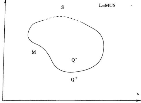
Figure 3.1: Simple closed curve on the complex plane
A further generalization of this problem is possible by introducing discon tinuous coefficients, A(zo)and B(zo) in (3.5). In addition, the behavior of X(z) at infinity can also be modified. For instance, it may also be described by a polynomial function of z. Let, the curve L be divided into two sets, M and S, such that MUS=L, as shown in Figure 3.1. Consider a boundary value problem of finding an analytic function X(z) with the boundary expressions
X + (zJ -f X-{zo) = 5 (z,), z, € M, (3.6)
X + { z , ) - X - { z , ) = 0 z ^ e S . (3.7) The two equations in (3.6) and (3.7) can be rearranged as a single one as
= F(.-„) (3.8)
bv introducing discontinuous coefficient and free term functions - 1 , ZoE M B (.-J = -|-1,
Z
q
G 6 B{zo), Zo € M (3.9) (.3.10) 0, Z(5 G 5"Note that equation (3.8) is valid on the whole closed contour L.
To make further derivations, it is necessary to specify the behavior of the unknown function X(z) at infinity and at the end points of the open curve
CHAPTER 3. MATHEMATICAL BACKGROUyD FOR RHP METH0DV2
M where A{z) and B{z) becomes discontinuous. It is assumed that X(z) has singularities of order 1/2 at each of the end points and is zero at infinity, which is a typical behavior for the electromagnetics problems of wave scattering and diffraction by perfectly conducting zero thickness slitted cylinders. However, the RHP technique can actually handle solutions with other singularities of the order less than 1, with nonzero behavior at infinity.
3.3
S o lu tio n o f th e R iem a n n -H ilb ert P ro b lem
By making the assumptions introduced in the previous section, we can define a function R(z), which is also called characteristic function, such that the multiplication of R(z) with X(z) becomes nonsingular everywhere, i.e. regular on the whole complex plane. It is given as
R(z) = (z - a, y /% z - a . y
/2
(3.11) where z=Qi,2 are the endpoints, and the branch is chosen such that brunch-cut is from a i to a2 along M. Then the limit values as c ^ ~o G M of R(z) differ by sign, i.e. R(z)-^· R^{zo) =By introducing functions Y(z) and D{zo) such that
D(z,) = B(zo)R+{=o) (3.13) we come to a RHP with continuous coefficient function on the closed curve L
Y U z o ) - y - { : : o ) ^ D { z . , ) . (3.14) Since the characteristic function has a simple pole at infinity, the solution of (3.14) is given as
The equation (3.15) can be written for the function X(z)
1 1 X{z) = L R+{zo)B{zO , ^ C -dzo -f R{z) (3.16) 2TviR{z)J\f {zo — z)
which is exact solution of the initial Riemann-Hilbert problem (3.6) and (3.7) with the restricted behavior of X(z) at the infinity and singularities of order 1/2 at the endpoints of the curve M.
CHAPTER 3. MATHEMATICAL BACKGROUND FOR RHP METH0D13
3.4
S olu tion o f C an on ical D u al Series E qu ation s
Consider the dual series equations with trigonometric kernel for the infinite sequence of coefficients Xn, n = 0 ,± l. ... , given as
OO ^ a-„|n|e·"^ = F(e·-'), € /U = (|s^| < 0) (3.17) /¿ = — OO OO x„e‘"^ = 0, ^ ^ S = { 0 < [ ^ \ <k). (3.18) 7l = — OO
Idiese dual series equations can be solved by converting the problem into a Riemann-Hilbert problem. Assuming that the series in (3.18) is term-by-term differentiable, we replace it with the derivative with respect to Then we have the following equations
n= — oc
= F(e‘"-),
V:> € M (3.19) OOE
n= —'X) Xnne"^^‘ - 0, ip G .S' (3.20) •X) (3.21) The last equation is obtained by substituting ip = w into (3.18) to account for the elimination of the constant term due to differentiation.By introducing functions A^*(z) of complex variable ~ - re“^ such that
OO X ^ { z ) = -I- ^ X n n z ’\ analytic in Q"*· = {·: : |~| < 1} 71— I -I X~{z) = - ^ Xnnz^, analytic in Q~ = [z \ l^l > 1} (3.22) (3.23)
we obtain a functional equation valid on the whole unit circle |;| A+(e·’^) - AX- { F^ ) = B
with known but discontinuous coefficient and free term functions - 1 , i pe M
(3.24)
A{ip) =
+ 1, € 5,
CHAPTER 3. MATHEMATICAL BACKGROUND FOR RHP METHODU
G M
0, G S. (3.26)
To arrive at the exact solution of (3.24), it is necessary to restrict the behavior of the unknown function X{z) at the infinity and at the end points of the screen. By assuming that X{z) vanishes as |i:| —> oo, and has a square root singularity at the endpoints, 2 = the solution is given by the equation (3.16). By using Plemelj-Sokhotskii formulas for the limiting values of the ,V(2), we obtain
in Js {t — to) dt + 2CQ{to) (3.27)
where tUo G L and
Q{to) = [/?+ (io)]-‘ , to G M
0, to G i>. (3.28)
The definition in (3.22) and (3.23) yields
X^{to) - X-[to) = ^ (3.29)
( n )
By taking the Fourier inversion of (3.29), we obtain
mxrn = Vm{F,6) + 2CRm{0), rn = 0, ± 1,... (3.30) where 1 f K (F ,e‘'^'-)e-'"‘'^" 2n Jo 2n J^M R+{C’^·'^) li.\, F(F,e''^") = —P.V. [ ' in Jm t — e"'’'" dt RAco^O)) =
The constant term in (3.27) can be found by setting rn = 0 in (3.30) as
v;
c =
-2Ro (3.31)
Assuming that the free term function has the Fourier expansion as F(F'^) = E / n e · ’^".
(n )
CHAPTER 3. MATHEMATICAL BACKGROUND FOR. RHP METH0D15
one can obtain
where VmiF,0) = J 2 f J Q (n) (3.33) 2irJM R+ie-^o)^ Vn{to,0) = - P . V . j I'x JM t — to (3.34) (3..3.5) Therefore, the equation (3.27) can be reduced to
where Xmm = - ^ f n V ^ (n) ,-n x.rn^m yn ^ yn _ y rn ’ m ' o R,-, (3.36) (3.37) One can find Xq as
- = - E / . E (-1)
(n)
(m^io)
Tti m
in
(3.3S)In terms of Legendre polynomials Pn(cos6) the results are as follows rn + 1
k
;(
cos«) =
-¡a,(cos«)a+i(cosO ) - P„+,(cosO)P„(cosO)|E ( - ‘r
m^O 2(m — n) 1 l/n yn-1 K lI(cos0) I -(l/n)I/„T\(cosi>), n 7^ 0 R m ( c O s 6 ) = ^P,n(cOS<?),m
l n l ± ^ n = 0 . (3.40) (3.41)Thus, the final solution to the canonical dual series equations obtained by the Riernann-Hilbert Problem method is found as
/n mzi(cO.S 0) (n)
(3.42) where Tmn{cos9) is given in the appendix.
The Riemann-Hilbert Problem method described above was first introduced in the diffraction theory by Agranovich, Marchenko and Shestopalov [.5] who applied it for solving a particular plane-wave scattering problem. Later, this method was expanded for a great variety of the scattering problems by many authors. A helpful survey of the approach with its application to a number of typical problems could be found in the work [8].
C h ap ter 4
R E F L E C T O R IN F R E E SPACE
4.1
Form ulation o f th e p rob lem
A general two-dimensional (2-D) reflector antenna geometry is shown in Figure 4.1. The perfectly-conducting reflector M is a part of a circle of radius a. The reflector has zero thickness and angular width 20ap with the central point at
Oo which is the offset angle. For a front-fed symmetrical reflector, Oo = 0.
Geometrical focus is located at the half distance of the circular radius a, h is the offset height, and 4’u are subtended angles to the lower and upper edges, respectively, tps is the half-angle subtended to the lower and upper edges, i.e.
(l/’y
-The radiation pattern of a directive line source feed is characterized by using the CSP method as described in chapter 2. It is known that main radiation beams of most antennas are Gaussian near the beam axis, and so. the idea of analytic continuation of the real source position to the complex space has been found to be extremely fruitful. In our structure, the source is placed at the geometrical focus, i.e., t^o = space, and its directivity is characterized by 6, so that the complex position vector becomes
rs = ro + ib = - cix + ibicos Ikij; -h sin iSuy). H-i:
The real number 6 is a measure of the feed directivity and the aiming angle /9 measured from the x-axis represents the beam direction. For the front-fed reflector case, /3 = 0.
Depending on the polarization, we denote by u{r) the //, or E. component of the field. The total field can be written as the sum of the incident
u'’'^{r) and the scattered fields. The incident field due to the line source 16
CHAPTER 4. REFLECTOR IN FREE SPACE 17
of amplitude C at the complex position is given by
= (4.2)
where k = uf c, and HQ^kr) is the Hankel function of the first kind (See section 2.1). With the use of the addition theorem for the Hankel functions, it can be written as
u '" ( r ,9) = C r > \ r - (4.:))
where
r, = y/j-Q + 'lirobcosß — 6^, ds = cos ‘ /_o_+_<6cos^ Re{r,) > 0.
(4.4)
For some geometries, the reflector surface may be in the near zone of the feed antenna, but the expression (4.3) is valid both at near and far zone of the feed as far as r > |rj| is satisfied. A note should be made that the function (4.2) is an exact solution of the Helmholtz equation; this is unlike Gaussian- type exponents frequently used to represent beam waves.
To obtain the rigorous solution of the problem, the scattered field has to satisfy the Helmholtz equation, the Neumann or Dirichlet type boundary con dition on the screen depending on the H or E-polarization, the Sommerfeld radiation condition, and the Meixner condition at the reflector edges. These requirements guarantee the uniqueness of the solution, and moreover, the ex istence in a certain class of functions [10, p.ll6], for any smooth open contour
A/.
CHAPTER 4. REFLECTOR IN FREE SPACE 18
The scattered fields can be expressed in integral form as a single-layer or double-layer potential over M. Then, imposing the boundary conditions, the following equations are obtained
and <9Я‘"(г) d f jH ^. . if r Í -= ~ д 7 , ] и <’ ■ '■ · '■ ^ ¿ 7 ( f . ?) = - í J^{7-')Go{C r’)dr'·. f G M J i\í
M
(T5) (T6)for II- and E-Polarization cases, respectively, where n is the outer unit normal, are the unknown current densities and G'o(c, r') is the 2-D Green's function (i.e., ¿/4//o^^(A-|r —r'D) and define the kernel of the integral e((uations.
Equations (4.5) and (4.6) are widely known, as well as the MoM-based solutions of them. It is worth noting that to reduce the singularity of the kernel, (4.5) can be transformed into a form similar to (4.6) [11, p.67j. However, conventional MoM solutions using sub-domain triangle or pulse basis functions lead to matrices of the order , V = l O D /A to ЗОЯ/A. A more reasonable choice of
basis functions, like a series of sinusoids as in [4]. may result in a much smaller matrix size; but it also increases the filling time drastically due to massive numerical integrations for matrix elements found as certain inner products. In general, as (4.6) is a Fredholm equation of the 1-st kind, it is ill-posed; and so the convergence of direct solutions to it is not guaranteed when /V —»· oo.
For these reasons, it is recommended to regularize (4.5) and (4.6), i.e.. to convert them to the Fredholm form of the 2-nd kind. .Л most straightforward way to achieve this is to make use of Tikhonov’s numerical self-regularization approach. This idea was exploited in [11] for a number of 2-D and 3-D axially- symmetrical open surfaces. Here, the convergence of MoM-type algorithms is ensured. Nonetheless, all the previous remarks about the matrix size (at least 10Я/А) and CPU time are valid.
The indicated problems can be overcome provided that the analytical reg ularization can be performed. The basic idea is of extracting a certain part of the integral operator which is invertible analytically, and inverting numerically the remaining part. Regularization ensures the existence of an exact solution and justifies application of a MoM-like numerical algorithm which is stable and has a pointwise convergence. .As for the efficiency, i.e., memory requirements and CPU time, it depends on the scatterer shape which determines the matrix elements. In case of M being an open circular contour, all the matrix elements can be obtained explicitly. This procedure is equivalent to a judicious choice
CHAPTER 4. REFLECTOR IN FREE SPACE 19
of basis functions in MoM-solution (as special scries of trigonometric functions [8, p.430]) possessing orthogonality, satisfying the edge condition in term-by- term manner and allowing to take inner-product integrals analytically. If the reflector is not circular, a similar approach can be developed but the matrix elements must be found by numerical integration. Thus, the advantages of the regularization in a circular geometry compel us to apply it to practical reflectors.
4.2
A p p ro x im a tio n o f a parabolic reflector by a circu
lar one
Parabolic reflector operation is based on the well known feature of the infinite parabolic surface to focus a plane wave to a certain fi.xed line. By reciprocity, if a line source is placed at the focal line, the secondary field has a planar wavefront independent of the polarization. However, if the reflector contour is only a part of a parabola, then the resulting edge spillover and diffraction cause the scattered field not to be a plane wave anymore. Instead, it is a cylindrical wave, and the total pattern contains a main beam and a number of sidelobes. To decrease the effect of edges, it is preferable to increase the reflector size, and to lower the amplitude of the primary field at the edges. In fact, this is the main reason for selecting a directive source as a feeder.
It is equally well known that if the focal distance F of a parabolic arc is large enough with respect to the reflector aperture D, this arc may be well approximated by a circular one, of the radius a = 2F [12]. Let us denote the radial deviation of such a circle from the parabola (i.e., the geometrical error) as A(t?) corresponding to the angular position 0. This function A monotoriically increases with 0, so that the maximum deviation is achieved at the reflector upper edge where 0 --- Oap + Oo. Further, this discrepancy between the parabola and the circle can be expressed in terms of the wavelength, A/A (this error can be called the electrical error). An engineering rule-of-thumb is that the errors smaller than A/16 = 0.06A may be neglected [13,1-1]. To illustrate. Figure 4.2 presents the family of equal-value curves of A /A in the plane of parameters
ka and O^p for a front-fed reflector. Also, the equal-value curves of the front-
fed aperture size D/X = {ka/r)s\nOap are presented for convenience. They indicate that the domain of validity in approximating a parabolic by a circular reflector is not restricted to electrically small reflectors. Indeed, in the case of a front-fed geometry, if Oap = 25° (a deep dish) one may take ka as much as
CHAPTER 4. REFLECTOR IN FREE SPACE 20
62, that IS D = lOA. However, if Oap = 15° (a shallow dish), the corresponding values expand to ka = 600 and D — 50A. For a practical offset reflector geometry where
0
q « Oap, an allowed aperture dimension is approximately half as large.4.3
D u al series eq uations for E and H p olarization cases
Guided by the considerations of the previous sections, we restrict our further analysis to the circular reflectors. The details of the regularization procedure has been published in [5-8]. Therefore, we shall concentrate on transforming the equation in a form suitable for an efficient numerical implementation. This is achieved by splitting the resulting matrix equations into two sets of equations corresponding to even and odd parts of the surface current.First, we discretize the integral equations (4.5) and (4.6) and reduce them to the series equations. Thus, for a circular contour M, the surface current densities are assumed to be zero on the rest of the circle (5), and expanded in terms of a series of angular functions with coefficients .r(/’^°, as follows
= C
^
t
n=-.=o
(4.7) where a n ~ l / k and «£; = 1 to account for the differentiation in (4.5). Sim ilarly, using the addition theorem, the Green’s function can be expressed in terms of a series of angular exponents. Then, substituting all the functions into (4.5) and (4.6), applying the boundary conditions over M, and taking ac count of the absence of the current on S', one obtains the following dual series eciuations.
For H-Polarization case,
oo oo
x!!j\(ka)ff!y(lca)c·"^ = - X: (4.8)
n= —OO n—— oo
f ; , r i V " '= 0 , v’ S.S, (4.9)
For E-Polarization case,
oo oo
■£ x ^ Mk a) H i'\ ka )e' ''' ^ =- Y , ^ € M, (4.10)
n=-oo n=--x»
CHAPTER 4. REFLECTOR IN FREE SPACE 21
Figure 4.2; Equal-value curves of the electrical error(A/A) and the reflector
size{D/\) as a function of ka and Oap. Solid curves represents constant reflector
CHAPTER 4. REFLECTOR IN FREE SPACE 22
where
b'J = (,« = (4.12)
and the prime denotes the derivative with respect to the argument.
4 .4
R H P solu tion and sy m m e try sp littin g
One can solve the dual series equations using the point-matching method [15]. However, as we have noted previously, that approach leads to an ill-posed equation set having no proof of universal convergence. Instead, vve extract a canonical form from the dual series equations which can be converted into a Riemann-liilbert Problem. Then, the analytical solution of the latter leads to a regularized infinite algebraic equation system of the Fredholm 2-nd kind differing from the plane-wave excitation case only by the right-hand part. In terms of the integral equations (4.5) and (4.6). this procedure is ecpiivalent to extracting and inverting the logarithmic part of the kernel function.
For H-polarization case, the regularized matrix equation is obtained as
n= —OO n = — C<j
and for E-polarization as
OO n=—oo
I 4 - È
(4.13) J,„[ka)Hÿi\ka) (4.14) where _ ^ F . U k a ) H i ' Hka) mn n J ^ { k a ) m n \ k a )The equation sets (4.1.3) and (4.14) obtained have summations going from —OO to +00. After truncation at the term they will have the order 2A’tr + f· To reduce the computation time, each of them can be splitted to two independent half-size equations. This is done by decomposing the problem into even and odd parts with respect to the symmetry axis of reflector. Indeed, introducing the even and odd expansion coefficients as
CHAPTER 4. REFLECTOR IN FREE SPACE 23
and substituting (4.15) into matrix equations, one obtains
CO
q ( W , £ ; ) . ± ^ ^ j ^{ H^E) , even/ odd^{H, E) , ± ^ E),even/odd^ ^ (0)1, 2, . . .
T i= ;(0) l
(4.16) where
(//) = ( - I ) ” ·"“!,*!/»!.®’ ± -4-™,.)·
even/odd ^ ^^(¿a)^ £ f^(H),even/odd(^_ .^^m+n ^ T^(„„),
n = (0) l
j ^ ( E ) , e v e n / o d d ______________________ n = (0) 1_________________________________________
" ~ Jrn(l-a)Hi!\L·)
with the coefficients and }}(E),even/odd follows
f^(H),even/odd ^ ^±(_ 1 ± ) ^{E),even/odd _ ^ J ) (4.17) (4.18) (4.19) (4.20) (4.21) (4.22) Here, is equal to and 7 “ is equal to unity where S„ is defined as 1 if n=0, otherwise 2. Other coefficients, T/[^ = Tmn{cosOap).T^^ = Tmn(-<^osOap) and the functions A f ,A^, Tmn, ^mn· are defined in the Appendix.
When solving a matrix equation, the CPU time is not a linear function of the matrix order. Therefore the reduction to two half-size eciuation sets saves the CPU time especially for large matrices, and also it avoids the inaccuracies resulting from the possible round off errors.
Note that in (4.16), the right hand parts have infinite summations that may lead to a certain truncation error in practical computations. The selection of new unknowns as
/4 " ’·* = 7 i A « a ! f '■* + i n t k a f b U r ’·'/-···· (4.23) A®’·* = 7i i »( 4») f f i ; ’( i < i ) A S o l f ' ( 4 - 2 4 )
modifies (4.16) to a form which enables one to minimize the truncation error in the right hand part. Eventually, any of obtained equations can be written
CHAPTER 4. REFLECTOR IN FREE SPACE 24
in the following operator notation
_ q(H.E),r:Vfnlode
where
Q{H),r.ven/odd ^
TTL \ / m
.evenlodd ^i^àir_i (L^\TT{l)ii
i,E),f:Vf.n/odd (4.25) ± r " ) (4.26) rf.nn) (4.27) in/odd (4.28) —1 L{E),cvtn/odd ^rn 1 (4.29)
I is the identity operator, and all the operators -4 are compact in the Hilbert
space of infinite sequences, /2 (i.e., with finite sum of squared absolute values of coefficients), see [8, p.430]. Hence, any of the operators / — A is of the Fredholm 2-nd kind in /2, and so Fredholm’s theorems are valid: provided that the right- hand part also belongs to /2, then the unique solution 3 exists in /2· Large- index estimates for cylindrical functions show that B G /> if Ic,! < a, resulting in a restriction a > 26/\/3 for front-fed primary line source. Furthermore, the approximate solution may be obtained with any desired accuracy via truncation to a finite order Ntr as the uniform pointwise convergence to exact solution is guaranteed for Ntr
00
.4.5
P h y sic a l O ptics so lu tio n
In the analysis of reflector antenna systems Physical Optics (PO) is a well known popular method[12,13]. PO uses Geometric Optic (GO) based currents, and generally gives better results for the mainbeam and the first few sidelobes of a parabolic reflector antenna. In the PO method, the radiation integral for the scattered field is calculated by employing the GO approximation for the currents induced on the reflector which is assumed to be electrically large. PO does yield useful estimates in directions where the GO currents produce the dominant contribution to the scattered fields. Results are obtained for both E and II polarization cases. Surface current is defined as Jpo =
2
?I x //" ' where ri unit normal vector to the surface of the reflector(See Figure 4.3) andis the incident magnetic field. Incident field depends on E or H polarization cases that is given as where p, is the complex position vector dependent on p which is the position vector from the source to the reflector surface.
CHAPTER 4. REFLECTOR IN FREE SPACE 25
Integral formulas are obtained for both E and H polarization cases as follows H-Polarization /~¡r , r / / , = 2\ / — / cos(o + ^/ 2) - — (4. 31) V bw y/r Jc y / ^ E-Polarization ^ i k r f. ^i kps E , = e‘T " / " V Ar Jc o s ( o ) + y s i n ( o ) ) ^ ^ (4.32) where P s = \Jp'^ - b ^ - 2t>6cos(0) ¡3 = K (4-33) and F ^ 4 /· (4-34) Surface current density is given by
g i /7 5
Jpo = 2 — ( 0 V F
(4.3.5)
Figure 4.3; Front fed symmetrical reflector antenna geometry Finally, integral equations become that
ikr .£)/2 ^ r c o s ( i + y / X ^ J - D / 2 ^ y /F s 2/ , Jkr ^D¡2 Jkp, /2 i,t/4 ^ / r___ (4.36) j , V ‘KP +"" dy (4.37) y/ÑrJ-D/2 y/ps
V
CHAPTER 4. REFLECTOR IN FREE SPACE 26
4.6
M e th o d o f M o m en ts so lu tio n
A method of moments solution is performed to compare the results for the circular screen with the RHP technique. Method of moments can be used in the solution of the small and medium size reflector antenna analysis. Although accuracy and convergence are not guaranteed, it may be practical to apply.
A simple solution is obtained by applying point-matching method to the cir
cular screen. Matching points are taken on the metallic and slot {>art of the circle.The following Dual Series Equations are used in the method of moments formulation. For H-Polarization n = -Ntr n=-Ntr /Vn
Z
n=-Ntr A e V- e M (4.3S) (4.39) For E-Polarization n = — Ntr n= — Ntr TlKp ^ e MZ
1· ^ " '· ’ = 0 € s n = - N t rwhere = Jn{krs)H[^^'{ka)e~"'^·' and 6^
--(4.40)
(4.41)
There are 2Ntr + ^ unknowns in the dual series equations. Therefore 2.V(,.-t-1 points at equal angles are taken on the circle of radius a to satisfy the equations (4.38).(4.39) or (4.40),(4.41).
4 .7
Far field ch a ra cteristics
The radiation pattern of the primary source is obtained from (4.2) or (4.3) by using large-Á;r asymptotic expansions of the Hankel functions. Similarly, one obtains the total field radiation pattern in the presence of the reflector as
r s j
CHAPTER 4. REFLECTOR IN FREE SPACE 27
where is taken as x^J'^{ka) or x^Jn{ka) depending on the H or E-polarization, respectively.
For the reflector antenna geometries, an important parameter is the total radiated power P normalized to the radiated j^ower Pq of the complex line source in free space. Pq is easily found by integrating the squared absolute value of the function (4.2) over the circle of a large enough radius ro| > > 1, and is given by
Po = C ^ ^ h C l k b ) (4.43)
k
where rj is (Zq)~^ and Zo for E and H-polarization cases, respectively. Zq is
the intrinsic impedance of free space and lo is the modified Bessel function of order 0.
Note that Pq increa.ses with kb rapidly as t^^^l\/kb. By following the for mulation of Section 2, the expression for P/Pq is obtained as follows
V - = ‘ + 7 7 í 7 ñ ê + (4.44)
The directivity D in the main beam direction (o = tt) is readily obtained as
- 1 ^
y~! C[Jn{kvs)e -f- ijn] (4.45)The frequency dependence of PjPq and D is important in designing the
narrow beam reflector antennas for pulse power transmission and wide-band communications. The directivity should be compared to the prime feed direc- tivitv. Dq, in the source beam direction {<f> = i) , which is easily found as
Dq = I0^{2kb)e^^\ (4.4G)
The ratio D / Dq shows the efficiency of the reflector as a directivity trans former.
C h ap ter 5
R E F L E C T O R IN S ID E A R A D O M E
5.1
R ad iation in th e p resen ce o f a circular radom e
To protect the reflector antenna systems from the environmental conditions, radomes are commonly used. The performance of the reflector antenna is changed by the presence of the radome, however almost distortionless trans mission is possible if the radome satisfies some electromagnetic requirements. Traditional techniques for the analysis of radomes, ray-tracing [17] and plane wave spectrum-surface integration (PWS-SI) [18] methods are based on the high frequency approximations. Both approaches depend on the local planar approximation for the curved interface reflection and transmission. The an tenna field at the radome walls are assumed to be a local plane wave nature as well as the radome wall is locally planar at the same point, d’herefore, both methods are used for a relatively large radome whose radii of curvature are large compared to wavelength.
In the PWS-SI technique [18], plane wave spectrum approach is combined with a surface integration procedure like physical optics or aperture integra tion. Multiple scattering by the antenna and radome is generally ignored and only fields on the radome surface lie in the forward halfspace of the antenna is considered. Ray-optical technique is one of the earliest methods. The aperture distribution is treated as a series of rays which are traced through the radome wall. In [19] and [20], ray-optical technique is extended to include the curva ture effects compared by the cylindrical radome of constant width. Radome prol)lerns can also be solved by the numerical methods like method of moments [21]. However, it is mainly limited to the small and medium size radomes.
In this section, radiation from a two dimensional circular reflector covered 28
CHAPTER 5. REFLECTOR INSIDE A RADOME 29
by a concentric and nonconcentric dielectric radome is analyzed by complex source-dual series approach. The solution is based on Riemann-Hilbert Prob lem technique, therefore unlike usual method of moments the results converge to the exact one in a pointvvise manner. The feed antenna is again modelled by the complex source point method.
5.2
C on cen tric radom e case
The geometry of the problem is two dimensional circular reflector surrounded with a concentric radome as shown in Figure 5.1. The reflector is modeled by a part of a circular, zero-thickness, perfectly conducting material of the radius ”a" and angular width ”20ap”· The feed antenna is located at the half distance of the circular radius ”a” and its beam is directed to the center of the symmetric front-fed reflector. Concentric radome of the relative permittivity
Cr and the permeability ßr covers the reflector system and its inner and outer
radius are given by ”c” and ”d”, respectively.
The requirements for the rigorous solution of the present boundary value problem can be stated as the satisfaction of the Helmholtz equation, Som merfeld radiation condition, edge conditions at the reflector edges and the boundary conditions on the conducting boundary and the boundaries of the circular radome.
CHAPTER 5. REFLECTOR INSIDE A RADOME 30
The basic electric field integral equations (EFIE) are obtained for both polarizations by applying the boundary conditions on the reflector part. These equations are dn and r\ ^ M , II-Polarization (5.1) / = —El’^{f) , r ^ M , E — Polarization (5.2) JM
where G’f, and are the Green’s functions for the layered medium and fi is the unit normal.
The Green’s functions for the single radome layer can be expressed as (5.3) (5.4)
where and G f are the free space Green’s functions for the z-directed mag netic (or electric) fields ci’eated by the line source located at the position (r'. <p) carrying a (^-directed (or z-directed) current. These functions can be written as - f) - ^ . (5.5) ’■') = '"'I =
E
. ’■ > n = — CO CO 6f (r-, r") = G ,(f. ,■') = »f.e·"·’ , .■ > / (5.6)where Go{r,7'') = — r'|) is the 2D free space scalar Green’s function. The expansion coefficients are given as
s i = . s i = . (-5.7) Let ^<n,E _ ST^ H\^\kor) d < r B ^ ’^ U k r ) + c < r < d A ^ ’^J„{kor) -I- a < r < c ^ IJV^ (5.8)
The expansion coefficients A^ ’^ a n d are evaluated by the application of the boundary conditions.
CHAPTER 5. REFLECTOR INSIDE A R A DOME 31
In order to reduce the integral equations (5.1) and (5.2) to the dual series equation, we substitute the discretized equivalent of the each integral parame ter. The surface current densities are e.xpanded in terms of a series of angular functions with Fourier series coefficients as follows
where an = I j k and a£; = 1.
irup (5.9)
Then the substitution of the discretized form of the surface current den sity, Green’s function and the incident field leads to the following dual series equations. H - Polarization case, n= —oo (5.10) oo = 0 , ^ € .s ri= —oo (.5.11) E - polarization case, oo oo n= —OO n= —OC' oo X; X f e - ^ = 0 , s^ € A / . (.5.12) (5.13) with X E = _JL q.
H,E H,E fH,E ,H,E
where .íl,E. ?1,E
gn “ in
(.5.14)
The functions appeared in the dual series equations are defined as
¡SH = J'^{koa)Hliy{Ka) - J'n{koafKl! 13^ = (J„(^,a)//<‘>(A-oa) - U k o a f K ^ r ' (5.15) (.5.16) = U k d ) H l ^ ^ k J ) - A;^’^V'„(A-d)//(‘)(A-od) (5.17) = Hi^\kd)H^;y{kJ) - k^y^H(;y{kd)H^^HkJ) (5.18)