MULTIVARIATE FORECASTING OF STEEL PRICES

(1)

T.C.

ISTANBUL AYDIN UNIVERSITY

INSTITUTE OF GRADUATE STUDIES

MULTIVARIATE FORECASTING OF STEEL PRICES

MASTER’S THESIS

Kaveh Ahmadi Adli

Department of Business

Business Administration Program

(2)

T.C.

ISTANBUL AYDIN UNIVERSITY INSTITUTE OF GRADUATE STUDIES

MULTIVARIATE FORECASTING OF STEEL PRICES

MASTER’S THESIS

Kaveh Ahmadi Adli (Y1812.130102)

Department of Business Business Administration Program

Thesis Advisor: Asst. Prof. Dr. Uğur ŞENER

(3)

DECLARATION

I hereby declare with respect that the study “Multivariate Forecasting of Steel Prices”, which I submitted as a Master thesis, is written without any assistance in violation of scientific ethics and traditions in all the processes from the project phase to the conclusion of the thesis and that the works I have benefited are from those shown in the Bibliography. (…/…/2020)

Kaveh Ahmadi Adli

(4)

FOREWORD

I owe my deepest gratitude to my supervisor Asst. Prof. Uğur Şener. Without his enthusiasm, encouragement, invaluable support, and constant optimism, this thesis would hardly have been completed. I would like to extend my sincere thanks to my parents and my sister for their continuous support and encouragement during all phases of my life. A very special word of thanks goes to my wife, who never let me down.

December, 2020 Kaveh Ahmadi Adli

(5)

MULTIVARIATE FORECASTING OF STEEL PRICES

ABSTRACT

Steel products are the most used raw material for many industries regarding their accessibility, strength, and relatively low costs comparing to the other base metals with similar characteristics. In the fast-paced economic environment of the post-world war II era with the growing expansion of the economy in the world, steel usage and consequently, the prices of steel become an essential concern for the countries and organizations. From the first decade of the 21st century, with the launch of the online trades for steel products in the commodity markets, the importance of steel prices has become even more critical. The practice of the price series forecast is conducted by various statistical and data-driven models in the literature. However, there is a lack of investigation to find practical and user-friendly statistical models in forecasting steel prices where, besides simplicity, can perform realistic and precise forecasts. The VAR and VEC models are newly introduced models comparing to the conventional models in econometrics. While the exogeneity in the conventional models can cause several difficulties in model specifications, the VAR systems, by treating all the variables as endogenous variables, can overcome this issue. Also, the VEC model that is a particular case of the VAR model, can assess the short-run and long-run dynamics by the cointegration relations in a single model. The data in this study are ranged from Jan. 2009 to Jun. 2020. The forecast evaluation is through the out-of-sample approach, which is more compatible with the real-world setting. The results of this study suggest the dominance of the VAR model over the VEC model in the forecast horizon of 18 months attributed to a mid-term forecasting horizon.

Keywords: Cointegration, Forecast, Multivariate, Steel, VAR, VEC

(6)

ÇOK DEĞİŞKENLİ TAHMİN MODELLERİNİN ÇELİK FİYATLARINA UYGULANMASI

ÖZET

Çelik dünyada yaygın olarak bulunan, dayanıklı ve benzer özelliklere sahip diğer ana metallere göre düşük maliyetli olma gibi üstünlükleri sayesinde özellikle üretim sektöründe en çok kullanılan hammadde haline gelmiştir. İkinci dünya Savaşı sonrasında hızla gelişen ve genişleyen ekonomik ortamda, çelik kullanımı ve dolayısıyla çelik fiyatları ülkeler ve kuruluşlar için önemli bir konu haline geldi. 21. yüzyılın ilk on yılından itibaren, emtia piyasalarında çelik ürünleri için çevrimiçi ticaretin başlamasıyla birlikte, çelik fiyatlarının önemi daha da artmıştır. Gittikçe önemi artan çelik fiyat serilerinin öngörüsü, literatürdeki çalışmaları göz önunde bulundurarak, çeşitli istatistiksel ve veriye dayalı modellerle yapılmaktadır. Ancak, basitliğin yanı sıra gerçekçi ve isabetli öngörüler yapabilen çelik fiyatlarına yönelik pratik ve kullanıcı dostu olan istatistiksel modellerinin kullanımının eksikliği literatürde görülmektedir. VAR ve VEC modelleri, ekonometride geleneksel modellere kıyasla, görece yeni tanıtılan modellerdir. Geleneksel modellerdeki dışsallık, model spesifikasyonlarında çeşitli zorluklara neden olabilirken, VAR sistemleri tüm değişkenleri içsel değişken olarak ele almaktadır. Ayrıca, VAR modelinin bir varyasyonu olan VEC modeli, tek bir model kulanarak, kointegrasyon yaklaşımına dayanarak kısa vadeli ve uzun vadeli dinamiklerini aynı zamanda değerlendirebilir. Bu çalışmada Ocak 2009 ve Haziran 2020 arasındaki aylık veriler kullanılmıştır. Tahmin değerlendirmesi, gerçeksel ortamla daha uyumlu olan, örneklem dışı yaklaşımla yapılmıştır. Bu çalışmanın sonuçları, orta vadeli olarak değerlendirilen 18 aylık öngörü ufkunda, LVAR modelinin VEC modeline üstünlüğünü göstermektedir.

Anahtar Kelimeler: Çok değişkenli Öngörü Modelleri, Çelik, Kointegrasyon, VAR, VEC

(7)

ABBREVIATIONS

ACF Autocorrelation function

ADF Augmented Dickey-Fuller

AIC Akaike Information Criterion

ANN Artificial Neural Networks

ARIMA Autoregressive Integrated Moving Average

ECM Error Correction Model

ECT Error Correction Term

FEVD Forecast Error Variance Decomposition

GDP Gross Domestic Production

IRF Impulse Response Function

ITC International Trade Commission

LME London Metal Exchange

Ln Natural Logarithm

LVAR VAR model on levels

MAE Mean Absolute Error

MAPE Mean Absolute Percentage Error

MSE Mean Square Error

NYMEX New York Mercantile Exchange

OLS Ordinary Least Square

PACF The Partial Autocorrelation Function

PPI Producer Price Index

(10)

RMSE Root Mean Square Error

SCI Schwarz information criterion

SSE Sum of Squared Errors

VAR Vector Autoregressive

VEC Vector Error Correction

VECM Vector Error Correction Model

(11)

LIST OF FIGURES

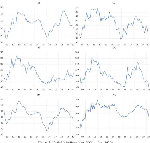
Figure 1: Variable Indices (Jan. 2009 – Jun. 2020) ... 30

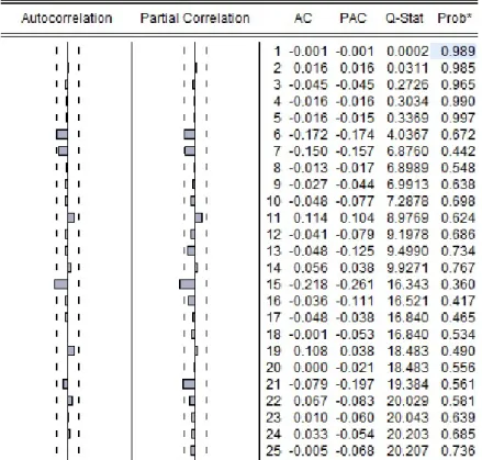
Figure 2: ACF and PACF for LnST Equation Residuals in the LVAR model ... 39

Figure 3: ACF and PACF for LnST Equation Residuals in the VEC model ... 39

Figure 4: IRF for the LVAR model ... 42

Figure 5: IRF for VEC model ... 43

Figure 6: Forecast Results from Jan.2019 to Dec.2020 ... 46

(12)

LIST OF TABLES

Table 1 Descriptive Statistics ... 29

Table 2 ADF test results ... 31

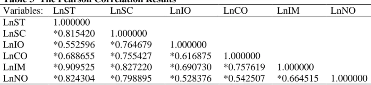
Table 3 The Pearson Correlation Results ... 32

Table 4 Granger Causality test for LnST variable ... 32

Table 5 Optimal Lag Length Selection Criteria ... 33

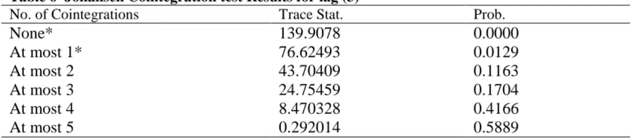
Table 6 Johansen Cointegration test Results for lag (3) ... 34

Table 7 LVAR (4) Estimation Results ... 35

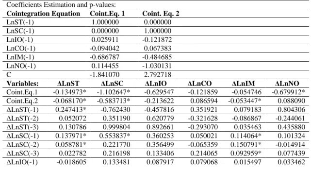
Table 8 VEC (3) Estimation Results ... 37

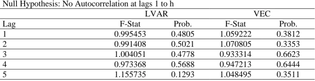
Table 9 The Result of the LM Test for LVAR and VEC Residuals ... 40

Table 10 The Result of the Heteroscedasticity Test for LVAR and VEC Residuals 40 Table 11 The FEVD of LnST for LVAR Model for 18 Months ... 44

Table 12 The FEVD of LnST for VEC Model for 18 Months ... 45

Table 13 Forecast Result values for 18 months ... 47

Table 14 Forecast Accuracy Measures for LnST ... 47

(13)

I. INTRODUCTION

A. History

Iron is the fourth element on the earth regarding redundancy, and about five percent of the earth's crust consists of iron. Initially, iron is manufactured around 2000 BC in southern Asia, which was the end of the bronze age. However, iron usage was expanded only after alloyed with carbon that has resulted in better characteristics compared to bronze. Subsequently, it is replaced by steel in mid-19th (Spoerl, 2004).

According to Verhoeven (2016), Mass scale production of steel started in the mid-19ths with the invention of the Bessemer process. New processes make it possible to produce cheaper steel. Andrew Carnegie – Industrialist – efforts to produce better quality cheap steel, lower the prices to $14 per ton in the late 19th century (Spoerl, 2004).

B. Importance of Steel and Its functions

Steel products are one of the essential intermediate commodities in the modern era, which results in economic growth and expansion. Everything we use is made of steel or steel equipment. In 2018, World crude steel production was reached an enormous amount of 1.87 billion tonnes with the apparent use of finished steel products for 1.76 billion tonnes (World Steel Association 2020). Nowadays, the usage of different types of steel products in a variety of industries such as construction, automaker, space, and aeronautics to the military, makes steel production a vital industry. Due to the high demand for steel, major labor force, and extensive facilities as national entities, the steel industry turns out to be politically and also economically significant (Jones, 2017).

Various steel applications can be seen as developed countries' foundation. Whereas economic growth is vital regarding making wealth and fulfilling the needs of people, the steel industry is among the industries which help to satisfy these

(14)

conditions. According to Dobrotǎ & Cǎruntu (2013), there is a positive relationship between economic growth and the production of crude steel in the aspect of GDP per capita. Furthermore, the technological advancement of a country can be predicted by the regime of steel usage.

The importance of steel consumption in the passenger car industry can be emphasized by the official reports show that more than 65% of an ordinary new car’s weight consists of steel and its components (Tilton, 1990). Referring to Bhat (2005), among the metallic materials, steel is the most widely used alloy in space exploration structures due to its excellent strength, flexibility, and low cost. Also, in the construction industry, all the buildings and structures mostly depend on steel for their rigidity.

Organization for Economic Co-operation and Development (OECD) Steel committee reported that up to 50% of steel consumption occurs in the construction industry, and the remaining half is divided almost equally between three industries: Transportation, Machinery, and Metal products. The Construction industry solely contributes to global GDP by 13% (OECD 2010).

C. Importance of Steel Price Forecasting

The prices are across the most demanding economic variables to predict (Popkin 1977). The importance of price specification in the business environment is unnegotiable, and it is the most critical factor for competitive advantage both at the corporate or country level. The Price forecasts can be used to diminish the ambiguity and help in the decision making process among organizations (Zarnowitz 1972). However, economic predictions boost assured establishment of strategies and investment plans in the long-term (Malanichev and Vorobyev 2011).

Generally, price forecasts are utilized as a tool for business activities such as budgeting, investment, risk analysis, and policymaking. Looking into the more comprehensive picture, it seems that price forecasting is the principal component of every financial planning. A proper plan, regardless of scope and duration, depends on forecasting. For emphasizing the importance of planning, General Eisenhower said: “Plans are nothing, but planning is everything.”

(15)

Regarding the knowledge that the future is the expansion of the present, thus making a reliable forecast, the past and present have to be assessed precisely (Szilágyi, Varga, and Géczi-Papp 2016). Price forecast is a useful skill for major establishments for planning as well as traders and small businesses to make a profit regarding knowledge about the price fluctuations.

Xia (2000) claims that the determination of steel prices has an essential role in the formulation of economic policy in less-developed countries. Robust steel prices forecasting has tremendous importance to specify and understand the steel market behavior and, consequently, for the industry to react in advance to fluctuations.

The London Metal Exchange (LME), as the largest commodity market for metals, has begun to trade steel since 2007. Consequently, the New York Mercantile Exchange (NYMEX) started to trade steel with future contract options. In these markets, most of the trades are made by future contracts that make steel a financial asset rather than a physical asset (Arık and Mutlu 2014). Since financial assets are prone to volatility, the forecasting of steel importance becomes critical for traders.

D. Insights About the Global Steel Industry and the United States

From the global steel industry’s data, it is observed a tremendous growth rate for crude steel production in the 1950-55 period with %7.4 as a reason for industrial recovery after the world war two economic crisis. In 1979 with the reforms applied to the Chinese economy to implement free-market rules, the country’s economic growth become the fastest in the world with an average real Gross Domestic Production (GDP) of 9.5% in 2018. China has become the world's most enormous steel producer and consumer with 927.5(%51.3) and 835.4(%48.8) million tons, respectively.

In the global steel industry, the ArcelorMittal company, based in Luxembourg, is the largest steel producer in the world, with 92.5 million tons of crude steel production following 76,033 million USD sales revenue, in 2018 which solely accounts for %5 of global crude steel production (ArcelorMittal 2019).

The U.S. was the world’s second largest steel product importer with a value of 23.9 billion USD in 2019. Canada, Brazil, Mexico, and South Korea are the major exporters to the United States. Also, the U.S. is the fourth major steel producer after

(16)

China, India, and Japan, with a total production of 87.9 million metric tons. Most steel production in the U.S. is made with iron and steel scrap instead of iron ore, which makes the scrap as an essential raw material in steel making. In recent years, the uncertainty in the steel market has increased due to the trade war between China and the U.S. that hit the steel market and complications related to the Covid-19 pandemic in the world.

E. The aim and scope

The current thesis aims to develop a proper multivariate model for forecasting steel prices. For explanatory variables, previous studies are considered in addition to some new variables which might affect steel prices as well. The models being used in this study are econometric models that use statistical analysis. The Vector

Autoregression (VAR) and Vector Error Correction (VEC) models, which are

extensions of George Box & Jenkins (1976), univariate Autoregressive Integrated

Moving Average (ARIMA) model are used for modeling purpose.

The forecast horizon is set to 18 months, which is equal to the average duration of future contracts in LME and NYMEX. whether in conventional markets or commodity exchanges, 18 months consider as an intermediate forecast horizon.

The upcoming chapters after chapter 1, that was the introduction, follow this structure; In chapter 2, available literature on the steel prices determination and forecasting is inquired in detail. Chapter 3 describes the methodologies that will be used for making models. Consequently, in chapter 4, data description and empirical results are included. Discussion and conclusion are fitted in chapter 6.

(17)

II. LITERATURE REVIEW

While economic forecasts play a significant role in policy decisions, the uncertainty in forecast results may lead the managers into erroneous conditions. While qualitative forecasts are relying on expert opinions and judgments, the quantitative forecast methods have developed under statistical knowledge consideration. The usage of statistical methods to model the financial and economic data which is called econometrics has an enormous part in limiting the uncertainty in forecasts. Econometrics has developed over the past decades as a result of the increasing calculation power in statistics. Also, the data classifications and preservice techniques make a significant contribution to economic and business data collections which then can be used with data-mining methods to simulate real-world conditions as well.

The globalization era which starts after world-war 2 initially, triggers the interest of the countries and companies over the world to trade internationally to boost their economic profile. However, regulating the suitable trade policy to support domestic industries while consolidating foreign trade has become a challenging task for the governments and policymakers.

China’s extraordinary economic growth results in the commodity market boom around the 2000s as a result of increasing demand. Subsequent recession in 2008 which pushes commodity prices downwards to the historical lows, makes pressure on the policymakers and business owners to have a clear perspective into the future to be able to mitigate the possible risks. Thus, forecast methods are started to use widely as a practical means to forecast commodity prices in various governmental and private financial institutions

The price forecasting process of a commodity involves the assessment of its characteristics and movements along with other commodities’ prices and some macroeconomic and microeconomic variables such as GDP, demand, supply, trade volume. Also, for intermediate commodities like steel which are made from other

(18)

commodities as raw materials, the current and historical prices of these commodities are essential.

Like any quantitative forecast process, it begins with the process of problem definition which describes the ultimate goal of forecasting. Subsequently, the data collection process takes part to collect suitable historical data which is assumed to be useful in forecasting the variable of interest for a proper time duration regarding the frequency of the data (e.g., annual, semi-annual, quarterly, monthly).

The next step is data manipulation since the raw data is not suitable to form a statistical method usually. In this stage, the most useful data considering their duration, predictability power, and characteristics are selected and transform into the desired format. The following step is the model building process which in this step a proper model is tried to fit the data. The model fitting process can be evaluated with model fit measurements to ensure the right specifications of the model.

After forming a proper model, it can be used to conduct a forecast using the same data as used in model fit (in-sample) or data that is kept off the modeling process (out-of-sample). The out-of-sample forecast is believed to yields more realistic and reliable results.

The last step in the forecast process is evaluation of the forecast to define the accuracy which is applied by comparing the actual values of the variable of the interest and its predicted values. This can be investigated by several forecast accuracy measures depend on the type and ultimate goal of the forecast.

Various studies are made an effort to forecast commodity prices; therefore, a few of them have tried to forecast steel prices. Also, existing literature about modeling steel prices is mostly concentrated on determining the steel prices structure in the market and not to forecast. However, price determination and forecast problems are overlapped most of the time, since the model which is made for price discovery can be used for price forecast with some considerations, practically.

The forecast problem in financial series is devoted to the two main categories as univariate and multivariate models. The univariate model depends on the variable of interest’s movements through time. In this manner, the forecast is performed by using the existing patterns in variables previous values which are used widely in the

(19)

literature for the price forecasting process for the short-term forecast horizons. However, due to the involvement of several microeconomic and macroeconomic factors, univariate models could not forecast longer horizons efficiently.

To overcome the problem of uncertainty by interventions and shocks initiated by other variables the multivariate forecast models are used. In multivariate analysis, the forecast model uses various explanatory variables besides the previous values of the interest variable to perform a forecast. Usually, the multivariate forecast can capture better results in mid-term and long-term horizons comparing univariate models.

To conduct managerial decisions and policy-making processes in organizations, mid-term and long-term forecasts are necessary, while short-term forecasts have vital importance for the traders in commodity markets. Therefore, as reviewed from the literature, univariate forecasts are less popular for macroeconomic forecasts as country scale or large organizations due to limited ability to conduct accurate long-term forecasts. The multivariate forecast models use leading variables that are efficient in forecasting the variable of interest.

The earliest and most known model for multivariate analysis is the Multiple

Regression model which the dependent variable regresses on the independent

variable(s). The estimation method for the coefficients in this model is the Least

Squares Method (LS). The development of the regression models allows us to include

the previous lags of the dependent variable and independent variables, as well. These models have belonged to the class of models which is popularized by George Box and Jenkins (1976) as Dynamic Regression (DR) or Transfer Function (TF) models. This class of models is also divided into several subsets and variations regarding some specifications in the modeling processes. The most essential ones are the

Distributed Lag (DL) model and the Autoregressive Distributed Lag (ARDL) model.

The ARDL model allows to include previous lags of the dependent variable besides the lags of the independent variables which is allowed in the DL model.

The assumption of the Exogeneity in the LS estimation method which articulates the independence of the explanatory variables with the error term becomes problematic in complex models with several explanatory variables. This difficulty is related to all variations of the DL models. The VAR model which is introduced by

(20)

Sims (1980), has overcome this issue by treating all variables as endogenous variables.

As an extensive issue in econometrics, the diversity and entanglement of the patterns in the time-series variables such as trend, unit-root, seasonal and irregular movements become complex and hard to distinguish. The problem arises where most of the econometrics models required decomposition of patterns in variables to analyze separately with multiple models. To prevail over this issue, the DL models required stationary (explained in detail in the methodology section) variables to form the model. The processes which are made to transform the non-stationary variables into stationary variables are entailed to some loss of information in the variables and have to be modeled by separate models.

Non-stationary variables are unstable in the mean due to the existence of the unit-root which by differencing the variables (subtraction of each value from the previous value) can become stationary. However, the differencing process eliminates the long-run dynamics of the variable due to removing stochastic trends in the variables. The financial variables are used to be non-stationary most of the time, and on the other hand, they need to be investigated for their long-run dynamics besides their short-run dynamics.

To overcome this dilemma, researchers suggested several models. therefore, the most successful and practical econometric models are VAR and VEC models. Engle and Granger (1987) study showed that the VAR model can handle the non-stationarity in the variables with consistent coefficient estimation. In addition, they introduced the new model based on the VAR model as the VEC model which separates the short-run and long-run dynamic of the variables by using the cointegration concept which is fully covered in the methodology section.

It is worth noting that the majority of studies used econometric models for determining and forecasting steel prices. Few recent studies used new data-driven models to assess and forecast steel prices, which the last one is back to 2015 by Liu, Wang, Zhu, & Zhang (2014).

In the following part of this chapter, firstly, a short brief is presented about the literature regarding methods and independent variables. Secondly, each of the related studies chronologically and methodologically is explained comprehensively. The

(21)

more weight is given to pieces of literature that used multivariate methods to assess or forecast steel prices.

Available studies offer a variety of explanatory variables, both globally and domestically. Among the different factors mentioned in these researches, raw materials cost, demand and supply, shipments, and foreign trade are seemed to be more efficient.

The majority of authors applied econometric models using regression analysis (Harmon, 1969; Liebman, 2006; Malanichev & Vorobyev, 2011; Mancke, 1968; Richardson, 1999; Xia, 2000). Kapl & Müller (2010) utilized the ARIMA and

Multichannel Singular Spectrum Analysis (M-SSA) methods. Chou (2013) used the

fuzzy time series analysis while Wu & Zhu (2012) and Liu et al. (2015) used Artificial Neural Network (ANN) to forecast steel prices. The forecast horizon varies from one step ahead to the multiple steps in the above studies.

Mancke (1968), as one of the earliest studies on the steel industry, tried to find an aggregate econometric model by using a multivariate linear regression method for the U.S steel prices from 1947 to 65. Since the steel is not homogenous material for finding the aggregate model, he investigated plates, sheets, and bars as the most used steel types in the industry. For independent variables, he described firstly the average variable cost, which represents all the costs depend on the amount of product, including raw materials, direct labor, etc. Secondly, imports are divided by total domestic production as an indicator of the market structure, which shows foreign competition on domestic products. Thirdly, the capacity utilization demonstrates the indirect relativity of demand to supply. He used dummy variables to differentiate years between 1947-1958, 1959-1965, 1947-61, and 1962-65 to learn about changes in the market condition. He found out that from 1947 to 58, steel prices tended to rise independent of demand and supply. However, from 1959 to 65, this condition has not been held. The second range of dummy variables which he assessed for governments guideposts effect on steel prices, there is no evidence to support this idea.

Grossman (1986) investigated the United States steel industry between 1976 and 1983, remarking the steel import prices, which were suggested to harm the country’s steel industry employment rate. This study proved that despite the assumption was made by the International Trade Commission (ITC) that imports are

(22)

the main reason for injury to the steel industry, other variables are more significant. He used several independent variables as time trend, industrial production, import prices, wages, price of energy and, price of iron ore to determine the effects on employment rate as the dependent variable in the multivariate regression. He concluded that the effect of industrial production as the indicator of changing demand is more than imports, which previously known as the main reason for damaging the steel industry.

In addition to Mancke (1968) and Grossman (1986) works in specifying the U.S. steel market, Blecker (1989) gave a comprehensive model to assess the steel industry between 1949 and 1983. In this work, the Dynamic Regression (DR) model was generated with steel prices as a dependent variable and cash dividends in product shipment, capacity utilization, import prices, market shares of four significant firms back at the time, overheads, and investments in the steel industry as independent variables. To avoid heteroscedasticity in the model due to outliers or omission of some variables, natural logarithm (ln) is used in regression analysis. He also tried to determine the demand quantity of the steel across the nation between 1954-83 regarding its impact on steel prices that it was included in the form of capacity utilization (CU) in the model. He ended that until the early 60’s because of the stable oligopolistic structure of the industry (price leadership by significant steel producers), prices did not depend on the demand or imports but depend on target-return pricing. However, after this time, steel prices responsive to demand and import competition. From the late ’60s, the demand starts to falling which, as stated in Grossman (1984), along with the growing import share, put downward pressure on steel prices.

Richardson (1999) investigated the effect of low-cost imports of steel from Eastern-European countries to the European Community (EC) between 1992-1994. After the 90s economic recession, as the start of the recovery phase, the steel demand in European countries was strengthened. The quarterly data are used for 12 years from 1981 to 1993 to form a model for steel price determination using multivariate linear regression.

A variety of explanatory variables as demand and potential supply capacity, cost structure, technology, price leadership, the exchange rate of ECU, surplus

(23)

capacity, inventories, and trade protection policies are investigated regarding effects on EC steel prices. Therefore, for the final model, he used the amount of import, apparent consumption, capacity utilization rates, and relative world price for cold-rolled coil steel as independent variables and Cold-Rolled Coil (CRC) steel prices for the EC as a dependent variable. R-squared (R2) statistics showed that independent

variables explain about 74% of CRC prices. In another equation, the import penetration ratio is used by dividing imports by apparent consumption against CRC prices. From the results, the author concluded that for 1 (million tonnes) of imports, the price cut-off by 50 ECU (European Currency Unit).

The master thesis by Xia (2000) gave insights about different factors other than demand and supply in determining steel prices in China from 1978 to1998. It is claimed that back in 20th-century, steel prices had been controlling by the government until 1993; hence the prices did not become sensitive to demand and supply. Five macroeconomic variables are introduced as explanatory variables, the Consumer Price Index (CPI), General National Product (GNP), which is the value of all finished goods and services in a country by its nationals in a given time period, exchange rate, interest rate, and the ratio of Import to Export of the country. The multivariate hedonic regression model with a lagged dependent variable as dummy variables. the data are transformed by natural logarithm (ln) to reduce the effect of the outliers. The result of empirical processes showed that only the ratio of import to export has a significant relation with the steel prices. Also, R-squared (R2) for this study explains about 60% of steel prices, which is not a satisfactory result. The research concluded that because of the manipulation of governments on the steel prices and lack of the equilibrium market price, all the factors except the ratio of the import to the export, show non-significant relations with steel prices. Therefore, it suggested that the model might be more suitable for countries with a free market.

Liebman (2006) is the most completed work done to investigate the U.S. steel industry. Following the previous studies, also Liebman studied the impact of safeguard tariffs on the steel industry by making the inclusive model for the steel industry. He considers seven different steel products monthly prices separately as the dependent variable from January 1997 to March 2005. As independent variables, industrial production index, iron ore, coal, steel scrap, industrial electricity price indexes, steelworkers wages in USD, the capacity index for steel production,

(24)

currency exchange rates for major steel exporting countries, time trend, steel demand for China, antidumping and, safeguards are considered in the multivariate regression model. The lagged data of 3, 6 and, nine months are used in this study to show the delayed effects of the independent variables on the steel prices. The distinction of this research from previous ones is including China’s growing demand in the model, which results in limiting producer countries’ capability to export to the U.S. and EU as the major importers of steel. With consideration to %98 (R2), the model looks appropriate for the designation of the U.S. steel market. The significant outcomes of this study are; first, the recovery of the steel industry in terms of prices had no statistical significance with safeguards as respected and Secondly, it is proved that the steel demand for china has a significant relationship with steel prices; therefore, after the retardation of six months.

The master thesis by Yuzefovych (2006) inspected the Ukrainian steel industry and compared it to the developed countries’ steel industries. The author aims to find out the consequences of joining the World Trade Organization (WTO) in the steel industry. She used monthly observations from 1999 to 2005. The method of the research is the Simultaneous Equation Model (SEM), which is used widely in econometrics when simultaneity is present. In this study, the price and quantity of steel production are two endogenous variables that depend on each other. Explanatory variables are used in the model are the quantity and capacity of the steel production, industrial production index of the EU, U.S., China, and Turkey, Gross National Product of the Ukrain (GNP), iron ore and coking coal prices. For obtaining results from the SEM model, two and three-stage least square (2SLS and 3SLS) estimations are used. The study proved that the Ukrainian steel industry had passed its transition stage, and there is a little risk of being hurt by joining WTO.

Following the studies on the U.S. steel industry as a primary importer of steel products, Blonigen, Liebman, & Wilson (2007) modeled the industry by econometric model. The research aims to find the ability of domestic steel producers to set a price above the marginal cost. To this aim, they used three equations in the SEM model as the quantity of demand, the quantity of import (supply) and, price. As explanatory factors index of industrial production, the real price of aluminum (as an alternative to steel), the exchange rate of exporter countries, other countries GDP, input prices (iron ore, metallurgical coal, oil) and, dummy variables to differentiate the period of

(25)

trade policies are used. For annual steel prices data, 20 different steel products from 1980 to 2006 are used. For calculating the three equation system, the three-stage least square method (3SLS) is used. The results are suggested that trade policies made to protect the steel industry were statistically insignificant, except for the 1980’s second half Voluntary Restraint Agreement (VRA).

In the paper published by Malanichev & Vorobyev (2011), they gave an effort to make a universal model for forecasting the global average annual steel prices based on the multivariate regression method. The forecast horizon was intermediate, which applied for the 2010-2012 period. The historical prices of the hot-rolled steel for four regions as the United States, Europe, China, and Russia from 1980 to 2009 were used as the dependent variable. For independent variables, Capacity Utilization, Raw Material Costs and, Time Trend is taken into the model. Capacity utilization is defined as the ratio of steel production divided by the steelmaking capacity of marginal producers around the world. Due to the equilibrium theory of demand and supply in the steel market, it is assumed that production (supply) is equal to consumption (demand), thus supply, demand and, steelmaking capacity explained by the dimensionless rate of capacity utilization. Raw material cost item is also determined by the weighted sum of iron ore and metallurgical coal usage per ton of steel. The authors claim that with the obtained model, for %7.5 growth in Capacity Utilization, the price of hot-rolled steel increases by 100 USD. Furthermore, increasing 1 USD in raw material costs results in an increase of 3 USD in hot-rolled steel prices. At the same time, the time trend presents a 5.2 USD decrease per each year due to the technological advancements in producing plants result in lower making costs. For the forecast of each independent variable in this study, a consensus forecast is prepared according to the global investment banks and specialized metallurgical agencies' reports for capacity and raw materials costs.

Recently with improvements in the computential power and expansion of new models, it has become possible to use sophisticated new models for economic indicators. Before these advancements, researchers mostly had been relied on conventional types of regression analysis to make forecast models. Some newer techniques, such as complex ARIMA based models, M-SSA. are used frequently with the help of software packages. Also, lately, the application of Machine-Learning Algorithms, especially Artificial Neural Networks (ANN), has made a tremendous

(26)

milestone in forecasting economic indicators. In the following paragraphs, some papers on forecasting steel prices with current methods will be described.

Kapl & Müller (2010) has compared the Auto-Regressive Integrated Moving

Average (ARIMA) with explanatory variables and a non-parametric spectral estimation model called Multi-Channel Singular Spectrum Analysis (M-SSA) for modeling and forecasting steel prices. For ARIMA with explanatory variables, lagged steel prices, lagged log of the coke prices, predictions of real GDP, lagged Dow-Jones index, and effectual exchange rates are used in the model. The M-SSA model is based on time series of hot-rolled coil prices, real GDP, index of the industrial production, the oil prices and, the Dow Jones stock index. It is concluded that while both methods have equivalent results regarding forecast error, the M-SSA method has larger amenability for generalization.

Chou (2013) worked on a model for long-term forecasting of global steel prices index through fuzzy time series, which was first introduced by Lotfi A. Zadeh in 1965. The author tried to make a forecast model for steel prices based on bulk shipping prices, Which are essential in the investment decision process for transportation companies.

Wu & Zhu (2012) attempted to predict steel prices for a week ahead through two univariate models. They utilized Radial Basis Function (RBF) Neural Networks and Adaptive Sliding Window (ASW) models using eight steel product prices from January 2011 to December 2011. For comparing two methods, Mean Absolute Errors (MAE) are used. The results proved that the ASW method is more suitable for forecasting steel market prices regarding forecast error.

Liu et al. (2014) used the Back Propagation Neural Network (BPNN) algorithm to forecast the steel prices index in China for the data from 2011 to 2013. The BPNN is a three-layer Feed Forward Neural Network (FFNN) that trains for errors by the Back Propagation algorithm. After correlation analysis was done for various factors, the iron ore price index, coke price index, and the average monthly trading volume of rebar steel are selected as inputs. For the output, the rebar steel price index is used. The article is concluded that the BPNN can forecast steel prices with excellent accuracy.

(27)

As a qualitative review study for the U.S. steel industry, Popescu et al. (2016) reviewed the effect of the steel imports on the U.S. steel industry. The study is pointed out some data about the crisis initiated by dishonest competition in the U.S. steel market as a result of the low-price steel products import.

Akman (2016) investigated the effect of the EUR/USD currency pair movements on the steel prices in Turkey as one of the largest steel producer countries. The study used the VAR model to determine the underlying relationship between pair currency relationship and steel prices.

As seen from the literature, there are limited researches that addressed forecasting in the steel industry, even though steel products are essential as physical and financial assets. One reason might be the overwhelming research enthusiasm about precious metals that can be beneficial in trades and result in the lesser notice for base metals. Another possible reason can be the unavailability of the data about the steel industry due to the strategic importance of the steel data for some countries.

The methodology which is used in most of the studies is econometric models. since econometric models comparing to data-driven models like the ANN and Fuzzy models can also reveal the underlying relationships among the variables besides the forecast process. Although, the ANN models might be able to forecast more accurately, therefore, due to black-box behavior, they unable to show the economic relationships which is the second most essential interest for econometricians and business forecasters.

(28)

III. METHODOLOGY

A. Definitions

Time Series and Stationarity

For describing the models that are used in this study, it is necessary to explain some fundamental definitions in time series analysis. According to George Box & Jenkins (1976), A collection of observations created sequentially in time order is called time series.

Time series can be stationary or non-stationary. In general, stationary time series are the ones that their pattern is independent of the observed time period. It means stationary time series should have a fixed mean and variance which do not vary with time (weak or wide-sense stationarity). There is another type of stationarity in time series which is called strict stationarity that requires covariance stability, besides mean and variance stability. However, this kind of stationarity is beyond the scope of the current study and not required in the models are used.

In another perspective, non-stationary time series is defined by random walks, drift, trend, and shifting variance. Defining time-series stationarity has a substantial role in econometric models.

Autocorrelation and Partial Autocorrelation Function

The Autocorrelation Function (ACF) is similar to correlation definition, which measures a linear relationship between two variables(series), while ACF assesses linear relationship within the variable with its time lags (Rob J Hyndman and Athanasopoulos 2018). The ACF is represented by equation 1.

𝑟𝑟

𝑘𝑘

=

∑ (𝑦𝑦𝑡𝑡−𝑦𝑦�)(𝑦𝑦𝑡𝑡−𝑘𝑘−𝑦𝑦�)

𝑇𝑇 𝑡𝑡=𝑘𝑘+1

∑𝑇𝑇𝑡𝑡=1(𝑦𝑦𝑡𝑡−𝑦𝑦�)2

(3.1)

Where T is the time period of the series, and k is the number of the lags.

The Partial Autocorrelation Function (PACF) is used with ACF in an association

to reveal patterns in the data. The PACF results in autocorrelation between the

(29)

current and kth lag while it controls the effects of other lags (Yaffee 1999). Both ACF and PACF play an essential role in identifying the characteristics of a time series. The patterns of ACF help to discover trends and seasonality in the time series.

Tests for Non-Stationarity

While with the contribution of the ACF and PACF, we can detect non-stationarity graphically; therefore, some tests are available to provide statistical evidence on the existence of the non-stationarity. There are several tests, including

KPSS, Dickey-Fuller (DF), Augmented Dickey-Fuller (ADF) and, Philips-Perron.

Despite its weaknesses, the most reputable non-stationarity test in literature is the ADF test, which is an extended version of the DF test.

The ADF test, which is introduced by Said & Dickey (1984), is the extension of the Dickey-Fuller (DF) test by Dickey & Fuller (1979) while allows detecting higher unit root order. The unit root is the characteristic of time series, which causes random walk (non-stationarity). The null hypothesis for the ADF test is that there is a unit root in the time series. The alternate hypothesis has three versions: 1) no unit root (random walk model), 2) no random walk with drift, 3) trend stationary. It means that if the test statistic is high enough regarding the significance level to reject the null hypothesis, then we can conclude that the time series is stationary. The test is using the principles of the Box-Jenkins Autoregression model.

Time Series Transformations

Most of the real-world financial time series represent non-stationarity, which in most cases they have to be converted to stationary series before applying in econometric models.

Weak stationary requires stability both in the mean and variance of the time series. Due to volatility and fluctuations resulted from seasonality and interventions in the financial time series, some transformations may be applied to stabilize the variance, such as natural logarithm, logarithm, square root, square, and Box-Cox transformations. Thus these transformations may render a time series into a series with finite variance (variance stability). In the literature, using the natural log for stabilizing the variance of financial series is a common practice.

(30)

For stabilizing the mean, the type of the trend(s) must be identified before try to render the time series into stationary. Since for stabilizing the mean, the trend may be modeled or eliminated. The determination of the trend can be done with the ADF test, considering the different variations of the test.

The deterministic trend is a result of the deterministic model, which gives the same result with given inputs in every implementation. Hence for de-trend, the deterministic trend first or higher-order regression equations may be used to model the deterministic trends. On the other hand, stochastic trends are the result of some stochastic process and cannot be modeled. To convert the time series into stationary series with the stochastic trend, first or higher-order differencing will be required. In differencing, each observation is subtracted from its own lag.

Generally, for the real-world settings, concerning the existence of both trends and fluctuations, a combination of transformations and de-trend or differencing may be used to render the time series into stationary.

B. Causality

The causality or cause-and-effect in statistics is referred to as the relationship whenever a variable’s lags affect another variable. The utilization of the causality in forecasting is based on the idea that cause cannot come after effect. Thus the determination of cause helps to improve the forecast in the target variable.

The concept of causality in economics initially introduced by Granger (1969) describes the effect of variable X’s lags on variable Y, and in contrast, the effect of variable Y’s lags on variable X. The Granger causality test procedure consists of two autoregressive equations that each equation tests for causality, based on other variables. The mathematical representation of the Granger causality is shown by equation (2).

𝑌𝑌

𝑡𝑡

= ∑

𝑛𝑛𝑖𝑖=1

𝛼𝛼

𝑖𝑖

𝑌𝑌

𝑡𝑡−𝑖𝑖

+ ∑

𝑛𝑛𝑗𝑗=1

𝛽𝛽

𝑗𝑗

𝑋𝑋

𝑡𝑡−𝑗𝑗

+ 𝑢𝑢

1𝑡𝑡

(3.2)

𝑋𝑋

𝑡𝑡

= ∑

𝑛𝑛𝑖𝑖=1

𝜆𝜆

𝑖𝑖

𝑌𝑌

𝑡𝑡−𝑖𝑖

+ ∑

𝑛𝑛𝑗𝑗=1

𝜎𝜎

𝑗𝑗

𝑋𝑋

𝑡𝑡−𝑗𝑗

+ 𝑢𝑢

2𝑡𝑡

λ

coefficients are statistically different from zero, we can conclude that each variable Granger causes other variables and vice-versa. Therefore, the null hypothesis for the Granger causality is no Granger causality, which means that the rejection of the null hypothesis proves the causality between the variables in each of the directions. Also, two-way causality (feedback) is possible between variables.

Due to the utilization of autoregressive equations, the assumption of the Granger test for variables is to be stationary. Hence in the case of non-stationarity, variables must be converted to the stationary process by differencing.

C. Vector Autoregression Model

The VAR model is an extension of the univariate ARIMA model that has the capability of multivariate analysis. The VAR model introduced by Sims (1980) is an attempt to solve the problems about the determination of the exogeneity for the variables in the conventional statistical model. Therefore, in the VAR model, all the variables are treated as endogenous variables, and there is an equation for each of the variables as an endogenous (dependent) variable. The model description for VAR is adopted from Enders (2014).

For simplicity, a bi-variate first-order VAR model is explained in the methodology part, which can be generalized for multiple variables as well.

We assume that Yt is being affected by the current and previous values of the Xt,

and in contrast, Xt is being affected by the current and past values of the Yt as well.

the formulation of the bi-variate model is shown in equations 3.3 and 3.4.

𝑌𝑌𝑌𝑌 = 𝑏𝑏

10

− 𝑏𝑏

12

𝑋𝑋

𝑡𝑡

+ 𝛼𝛼

11

𝑌𝑌

𝑡𝑡−1

+ 𝛼𝛼

12

𝑋𝑋

𝑡𝑡−1

+ 𝜀𝜀

𝑦𝑦𝑡𝑡

(3.3)

𝑋𝑋𝑌𝑌 = 𝑏𝑏

20

− 𝑏𝑏

21

𝑌𝑌

𝑡𝑡

+ 𝛼𝛼

21

𝑌𝑌

𝑡𝑡−1

+ 𝛼𝛼

22

𝑋𝑋

𝑡𝑡−1

+ 𝜀𝜀

𝑥𝑥𝑡𝑡

(3.4) Where b10 and b20 are constant term for equations, Yt and Xt are stationary

seriesand 𝜀𝜀_{𝑦𝑦𝑡𝑡} and 𝜀𝜀_{𝑥𝑥𝑡𝑡} are white-noise residuals, which means there are no patterns that exist in the residuals after modeled by the equations. Equations 3.3 and 3.4 cannot be estimated directly through Ordinary Least Square (OLS). Due to the inclusion of the current value of Xt in the Yt’s equation and vice-e-versa, which

makes the residuals of the two equations correlated. Consequently, the correlation of

(32)

residual terms results in the system’s bias and violates the assumption of the independent residuals for the OLS system.

For this reason, a transformation of the system through matrix algebra is needed to solve this problem. The matrix representation of the above two-equation system is demonstrated in equation 3.5.

� 1

_𝑏𝑏

𝑏𝑏

12 21

1 � �

𝑌𝑌

𝑡𝑡

𝑋𝑋

𝑡𝑡

� = �𝑏𝑏

10

𝑏𝑏

20

� + �

� + �

𝜀𝜀

𝑦𝑦𝑡𝑡

𝜀𝜀

𝑥𝑥𝑡𝑡

�

(3.5)

Or we can write as equation 3.6.

𝐵𝐵𝐵𝐵

𝑡𝑡

= Γ

0

+ Γ

1

𝐵𝐵

𝑡𝑡−1

+ 𝜀𝜀

𝑡𝑡 (3.6) Where: 𝐵𝐵 = �

_𝑏𝑏

1 𝑏𝑏

12 21

1

�

,

𝐵𝐵

𝑡𝑡

𝑡𝑡−1

+ 𝑒𝑒

𝑡𝑡 (3.7) Where

A

₀

= 𝐵𝐵

−1

Γ

₀

,

A

₁

= 𝐵𝐵

−1

Γ

₁

,

and

e

_𝑡𝑡

= 𝐵𝐵

−1

𝜀𝜀

_𝑡𝑡

.

With assigning 𝑎𝑎_𝑖𝑖0 as the element of the vector A₀, 𝑎𝑎_{𝑖𝑖𝑗𝑗} as the element of the matrix A₁ with (i) for rows and (j) for columns and, 𝑒𝑒_{𝑖𝑖𝑡𝑡} as the element of the vector 𝑒𝑒𝑡𝑡 the VAR model can be formed as equations 3.8 and 3.9.

𝑌𝑌𝑌𝑌 = 𝑎𝑎

10

+ 𝑎𝑎

11

𝑌𝑌

𝑡𝑡−1

+ 𝑎𝑎

12

𝐵𝐵

𝑡𝑡−1

+ 𝑒𝑒

1𝑡𝑡

(3.8)

𝐵𝐵𝑌𝑌 = 𝑎𝑎

20

+ 𝑎𝑎

21

𝑌𝑌

𝑡𝑡−1

+ 𝑎𝑎

22

𝐵𝐵

𝑡𝑡−1

+ 𝑒𝑒

2𝑡𝑡

(3.9)

While equations 3.3 and 3.4 are called the structural VAR and contain current values of the variables, equations 3.8 and 3.9 are called reduced-form or standard form VAR.

(33)

In order to form a VAR model with multiple variables, the same methodology is used as well. The matrix representation of the VAR model for multiple variables is reported in equation 3.10.

�

𝐵𝐵

1𝑡𝑡

𝐵𝐵

2𝑡𝑡

_.

𝐵𝐵

𝑛𝑛𝑡𝑡

� = �

𝐴𝐴

10

𝐴𝐴

20

_.

𝐴𝐴

𝑛𝑛0

� + �

𝐴𝐴

.

𝐴𝐴

𝐵𝐵

2𝑡𝑡−1

_.

= 𝛿𝛿 + ∑

𝑃𝑃

𝛤𝛤

_𝑖𝑖

𝐵𝐵

_{𝑡𝑡−𝑖𝑖}

+ 𝑒𝑒

_𝑡𝑡

𝑖𝑖=1

(3.11)

Where 𝐵𝐵_𝑡𝑡 is (N × 1) vector of endogenous variables,

𝛿𝛿

is (N × 1) constant term vector,

𝛤𝛤

_𝑖𝑖 is (N × N) matrix of coefficients, and

𝑒𝑒

_𝑡𝑡 is (N × 1) vector of the white noise residuals.

The estimation for the VAR model is OLS, which means each equation in the VAR system can be estimated using OLS. Residuals in OLS estimation are assumed to be not autocorrelated, in addition to the constant variance.

Selection of optimal lag length (P) in the VAR process is made with consideration to information criteria like Likelihood Ratio (LR), Akaike’s Final

Prediction Error (FPE), Akaike Information Criterion (AIC), Schwarz information criterion (SIC), or Bayesian Information Criterion (BIC), and, Hannan-Quinn Information Criterion (HQ). However, Lütkepohl (2005) suggested that selecting

optimal lag length is not a crucial point when the primary goal of the modeling is just forecasting. For the model fit, Gredenhoff & Karlsson (1999) showed that AIC performs more favorable results rather than rivals.

The AIC is being used in the current study for selecting the optimal lag length, and the basic formula is demonstrated as equation 3.12.

𝐴𝐴𝐴𝐴𝐴𝐴 = −2(𝑙𝑙𝑙𝑙𝑙𝑙 − 𝑙𝑙𝑙𝑙𝑙𝑙𝑒𝑒𝑙𝑙𝑙𝑙ℎ𝑙𝑙𝑙𝑙𝑜𝑜) + 2𝐾𝐾

(3.12)

(34)

The log-likelihood is a natural logarithm transformation of the likelihood function, which is used to assess the integrity of the model to the data. K is the number of model parameters, including the intercept.

D. Cointegration and Vector Error Correction Model

Initially, for describing the cointegration, the integration order I(d) and economic equilibrium have to be explained.

In order to transform the nonstationary time series with unit root to stationary series, the differencing is needed. The number of differences is defined by I(d), which d is the order of integration. In economics, the Equibilirium or Market-clearing is a situation in which economic forces (e.g., price, demand, supply), in the lack of external interventions, remain in balance.

_𝑡𝑡

= 𝑧𝑧

_𝑡𝑡 (3.14) Where 𝑧𝑧_𝑡𝑡 is assumed as a stochastic variable that indicates the departure from the long-run equilibrium. If all components of 𝑦𝑦_𝑡𝑡 are integrated of order (d), and a linear combination exists as: (𝛽𝛽′𝑦𝑦_𝑡𝑡 = 𝑧𝑧_𝑡𝑡) with β = (β₁, . . . , 𝛽𝛽_𝐾𝐾)′ ≠ 0, then it can be

(35)

possible that 𝑧𝑧_𝑡𝑡 is the cointegration relationship between variables with the order of integration I (d-b). Also, the vector β is named the cointegration vector, which is not exclusive, since it can be possible to have multiple linearly independent cointegrated vectors.

There are two approaches to test the cointegration among variables. First, the Engle & Granger (1987) test procedure, which can only demonstrate single cointegration between two variables with a single equation model, as another option, the Johansen test procedure was introduced by Johansen (1991) and Johansen & Juselius (1990), which can be more practical since it can be used for several variables and unveils more than one combination of the cointegration vectors among the variables.

The Johansen procedure uses two types of tests as Trace, and Maximum

Eigenvalue tests, which the former is from the linear algebra, and the ladder is a

scalar. The null hypothesis for both tests is in favor of no cointegration among variables. The difference between these tests arises in the alternate hypothesis. The Trace test alternate hypothesis is that there is at least one cointegration combination. The Maximum Eigenvalue test alternate hypothesis is that there is a cointegration combination with the addition of one (K0+1).

According to the literature, the Trace test in Johansen Procedure performs better than the Maximum Eigenvalue test, mainly when it is suspected to have more than one cointegration combinations (Cheung and Lai 2009; Lütkepohl, Saikkonen, and Trenkler 2001).

The assumption for the Autoregressive (AR) model, which also the VAR model is based on, is that variables have to be stationary. For the VAR model to be stationary, the roots (coefficients) should be outside the unit root circle of the equations embedded in the VAR system. The majority of the economic variables are non-stationary variables which transforming them into stationary process result in the loss of some critical features of the variable like trends and long-run relationships. Thus, performing the VAR model with differenced data expels the plausible long-run relationship among the data.

In the literature, it is discussed that the VAR system can handle the non-stationarity by running on level variables (LVAR), which in this case, it gives

(36)

consistent parameter estimation without eliminating the long-run dynamics in the cointegrated variables (Phillips and Durlauf 1986; Sims, Stock, and Watson 1990; West 1988).

For modeling cointegrated variables considering both short-run and long-run dynamics, the Error Correction Model (ECM) was introduced by Engle & Granger (1987), which is a particular case of the VAR model. This is a two-stage model with a single equation along with the endogenous variable and multiple exogenous variables, which allows for one set of cointegration to be modeled. Another approach is Johansen’s Vector Error Correction Model (VECM) by Johansen (1991), which uses the VAR model to formulate the numerous cointegrations (long-run dynamics) along with the short-run dynamics as well.

The two variables system is used to explain more straightforwardly for the ECM model in equations 3.15 to 3.17. Assume that the long-run relationship (equilibrium) between two variables is:

𝑦𝑦

1𝑡𝑡

= 𝛽𝛽

1

𝑦𝑦

2𝑡𝑡

(3.15) Where the alterations in 𝑦𝑦_1𝑡𝑡 , based on departures from the equilibrium in the previous period (t-1). We use the differenced variables, which are represented by the Δ sign.

∆𝑦𝑦

1𝑡𝑡

= 𝐴𝐴

1

�𝑦𝑦

1,𝑡𝑡−1

− 𝛽𝛽

1

𝑦𝑦

2,𝑡𝑡−1

� + 𝑢𝑢

1𝑡𝑡

𝑡𝑡−1

+ 𝛤𝛤

1

∆𝑦𝑦

𝑡𝑡−1

+ 𝑢𝑢

𝑡𝑡

(3.19) Where: 𝑦𝑦𝑡𝑡= (𝑦𝑦1𝑡𝑡, 𝑦𝑦2𝑡𝑡)′, 𝑢𝑢𝑡𝑡 = (𝑢𝑢1𝑡𝑡, 𝑢𝑢2𝑡𝑡)′, 𝐴𝐴 = �𝐴𝐴_𝐴𝐴1 2�, 𝛽𝛽 ′ _{= (1, −𝛽𝛽} 1), and

𝛤𝛤

1

= �

𝛾𝛾

_𝛾𝛾

11,1_21,1

_𝛾𝛾

𝛾𝛾

12,1_22,1

�

The VEC model with intercept term can be written with the help of some algebraic modifications and simplifications by using matrix notation, as:

∆𝐵𝐵

𝑡𝑡

= 𝛿𝛿 + ∑

𝑃𝑃−1𝑖𝑖=1

𝛤𝛤

𝑖𝑖

∆𝐵𝐵

𝑡𝑡−𝑖𝑖

+ 𝛱𝛱

𝑦𝑦𝑡𝑡−1

+ 𝑒𝑒

𝑡𝑡

(3.20)

Where 𝐵𝐵_𝑡𝑡 is (N × 1) vector of endogenous variables, 𝛿𝛿 is (N × 1) constant term vector, 𝛤𝛤_𝑖𝑖 is (N × N) matrix of coefficients for short-run dynamics, Π is the matrix of coefficients for Error Correction Term (ECT), and 𝑒𝑒_𝑡𝑡 is (N × 1) vector of the white noise residuals. The ECT demonstrates the speed of correction towards the long-run dynamics due to the interventions. While the Negative ECT sign shows the convergence of the shock along with the equilibrium, the positive sign demonstrates explosive or divergence behavior. It is important to notice that the lag length criteria which is determined in VAR (p) model is also applicable to VEC model with (p-1) since lagged differences in VEC model represent to VAR (p) (Lütkepohl 2005a).

Unlike the VAR model on levels (LVAR), the VEC model differentiates the short-run dynamics from the long-run dynamics. The VEC model uses differenced variables to investigate the short-run, and it includes the cointegration equation to the model to assess the long-run dynamics.

According to Shoesmith (1995), some problems occur in the case of multiple cointegrations presence 1

. Mostly, it becomes more problematic when these cointegration relationships are not compatible with economic theories. However, despite these problems, using any combination of cointegration relationships may improve the forecast accuracy as well (Shoesmith 1995a).

1_{See (Shoesmith 1992, 1995a) for more details}

25

(38)

E. Impulse Response Function

For investigating the interactions among the variables, in addition to the Granger causality analysis, the Impulse Response Function (IRF), which is generalized by Pesaran and Shin (1998) is used as well. The IRF shows the reaction of the variable of the interest to exogenous shocks or interventions, which usually are called shocks in the economics literature. Often the IRFs are modeled in the context of the VAR and VEC models, where regardless of the endogenous description of these systems, impulses are treated as an exogenous variable to the response in the variable of the interest.

Usually, the IRF is formulated as the Vector Moving Average (VMA) representation of the VAR model as equation 3.21.

𝑦𝑦

𝑡𝑡

= 𝛿𝛿 + ∑

∞𝑖𝑖=0

𝛩𝛩

𝑖𝑖

𝜀𝜀

𝑡𝑡−𝑖𝑖

(3.21)

Where the components of the 𝜀𝜀_𝑡𝑡 are independent, which are representative of the MA process. The 𝛿𝛿 is the intercept term. The unit of a shock in each component is one standard deviation.

F. Forecast Error Variance Decomposition

The Forecast Error Variance Decomposition (FEVD) is another tool to investigate the interconnections among multiple variables in the VAR or VEC models. The FEVD indicates the proportionated movements through the time, based on the variable’s own shocks against other variables shocks (Lütkepohl 2005b). In a VAR model, the FEVD shows the proportional contribution of each variable to forecasting the variable of interest. For estimation of FEVD, the Mean Squared Error (MSE), as a forecast error measurement along with MA representation of the process, is used. The equation to estimate the FEVD is illustrated as 3.20.

𝜔𝜔

𝑗𝑗𝑘𝑘,ℎ

= ∑

ℎ−1𝑖𝑖=0

(𝑒𝑒′

𝑗𝑗

𝛩𝛩

𝑖𝑖

𝑒𝑒

𝑘𝑘

)

2

/𝑀𝑀𝑀𝑀𝑀𝑀�𝑦𝑦

𝑗𝑗,𝑡𝑡

(ℎ)�

(3.22) The 𝜔𝜔_{𝑗𝑗𝑘𝑘,ℎ} is the proportion of the h-step FEVD of the variable j comprised of

interventions or shocks in variable k.

MULTIVARIATE FORECASTING OF STEEL PRICES

T.C.

ISTANBUL AYDIN UNIVERSITY

INSTITUTE OF GRADUATE STUDIES

MULTIVARIATE FORECASTING OF STEEL PRICES

MASTER’S THESIS

Kaveh Ahmadi Adli

Department of Business

Business Administration Program

DECLARATION

FOREWORD

ABSTRACT

ÖZET

TABLE OF CONTENTS

ABBREVIATIONS

LIST OF FIGURES

LIST OF TABLES

I.

INTRODUCTION

II.

LITERATURE REVIEW

III.

METHODOLOGY

𝑟𝑟

=

𝑌𝑌

= ∑

𝛼𝛼

𝑌𝑌

+ ∑

𝛽𝛽

𝑋𝑋

+ 𝑢𝑢

𝑋𝑋

= ∑

𝜆𝜆

𝑌𝑌

+ ∑

𝜎𝜎

𝑋𝑋

+ 𝑢𝑢

α

σ

β

λ

β

λ

𝑌𝑌𝑌𝑌 = 𝑏𝑏

− 𝑏𝑏

𝑋𝑋

+ 𝛼𝛼

𝑌𝑌

+ 𝛼𝛼

𝑋𝑋

+ 𝜀𝜀

𝑋𝑋𝑌𝑌 = 𝑏𝑏

− 𝑏𝑏

𝑌𝑌

+ 𝛼𝛼

𝑌𝑌

+ 𝛼𝛼

𝑋𝑋

+ 𝜀𝜀

� 1

𝑏𝑏

𝑏𝑏

1 � �

𝑌𝑌

𝑋𝑋

� = �𝑏𝑏

𝑏𝑏

� + �

𝛼𝛼

𝛼𝛼

𝛼𝛼

𝛼𝛼

� �𝑌𝑌

𝑋𝑋

� + �

𝜀𝜀

_𝑏𝑏

_𝑏𝑏