ARI (1999) 51 : 268}276 ( Springer-Verlag 1999
O R I G I N A L A R T I C LE
N. S. S,engoKr' Y.xak1r' C. GuKzelis, ' F. Pekergin OG. MorguKl
An analysis of maximum clique formulations and
saturated linear dynamical network
Received: 18 March 1999/Accepted 26 April 1999
Abstract Several formulations and methods used in solv-ing an NP-hard discrete optimization problem, maximum clique, are considered in a dynamical system perspective proposing continuous methods to the problem. A compact form for a saturated linear dynamical network, recently developed for obtaining approximations to maximum clique, is given so its relation to the classical gradient projection method of constrained optimization becomes more visible. Using this form, gradient-like dynamical systems as continuous methods for "nding the maximum clique are discussed. To show the one to one correspondence between the stable equilibria of the saturated linear dynamical network and the minima of objective function related to the optimization problem, La Salle's invariance principle has been extended to the sys-tems with a discontinuous right-hand side. In order to show the e$ciency of the continuous methods simulation results are given comparing saturated the linear dynam-ical network, the continuous Hop"eld network, the cellular neural networks and relaxation labelling net-works. It is concluded that the quadratic programming formulation of the maximum clique problem provides a framework suitable to be incorporated with the continu-ous relaxation of binary optimization variables and hence allowing the use of gradient-like continuous systems which have been observed to be quite e$cient for minim-izing quadratic costs.
N. S. S,engoKr ( ) ' Y.hakmr' C. GuK zelis, Department of Electronics and Communication, Istanbul Technical University, Maslak 80626, Istanbul, Turkey
e-mail: [email protected], Tel.: #90 212 285 36 19, Fax.: #90 212 285 36 79 F. Pekergin
LIPN-University Paris Nord, 93430-Villetaneuse, France OG. MorguKl
Bilkent University, Bilkent, Ankara, Turkey
This work was supported by TUGBITAK-CNRS, Turkish and French Scienti"c and Technical Research Councils
Key words Optimization ) Maximum clique problem ) Continuous methods ) Gradient systems )
Gradient-projection algorithm ) Discontinuous di!erential equations ) La Salle's invariance principle
1 Introduction
The maximum clique problem is to "nd a maximum complete subgraph of a graph. This graph theoretical problem is computationally equivalent to some other graph theoretical problems such as the maximum inde-pendent set and minimum vertex cover problem. The maximum clique problem and its equivalents are NP-hard optimization problems. However, it is essential to "nd the solution to them since these problems have theoretical and practical importance and are encountered in a diverse domain. The simplest method of "nding the largest clique is to test all subsets of the vertices of a graph to see if they induce a complete graph. In the worst case, this method of solving the problem will give rise to a computing time that will exponentially grow with graph size. So in order to cope with its NP-hardness, di!erent formulations and di!erent algorithms have been used to solve the maximum clique problem and its equivalents. A complete review of the formulations and algorithms developed can be found in Pardalos and Xue (1994), Pelilo (1995), Jagota (1995) and Pekergin et al. (1998). In Pardalos and Rogers (1992), the problem is formulated as an unconstrained quadratic 0}1 program. In Pardalos and Rogers (1992), it is also given in a linear programming formulation with a unit simplex feasible region. In the papers that aim to solve maximum clique and equivalents in the neural network domain (Pelilo 1995, Jagota 1995, Funabihi et al. 1992, Grossman 1995, S,engoKr et al. 1998), energy descent opti-mizing dynamics are used. Yet another work is Pekergin et al. (1998) which bene"ts the saturated unstable linear dynamics. It is shown in Pekergin et al. (1998) that, for almost all initial conditions, any solution of this saturated
linear gradient dynamical network de"ned on a closed hypercube reaches one of the vertices of the hypercube and any reached vertex corresponds to a maximal clique. In recent years, there has been an interest in approaches based on continuous optimization. One of the main pur-poses of this paper is to show with a particular emphasize on the maximum clique problem, that gradient and gradi-ent-like systems present e$cient continuous solution methods for quadratic discrete optimization problems, and that the dynamical system theory provides a useful framework for analyzing such continuous methods and many others. Gradient dynamical systems can be de-scribed in a state equation from whose vector "eld is produced by the gradient of a scalar function, called energy. Energy descent and convergence properties of its completely stable equilibria to which trajectories converge correspond to local minima of the cost function. So called gradient-like systems covering quasi-gradient systems in Chiang and Chu (1996) and many dynamical neural net-works (as special cases) which are in fact not gradient systems, but they also have the same kind of dynamics, can be used for minimizing cost functions with continuous optimization variables. It should be noted that the con-tinuous Hop"eld network (Hop"eld 1982), the Grossberg neural network (Grosberg 1976), and the cellular neural network (Chua and Yang, 1988) are of gradient-like sys-tems and are used for solving several optimization problems. Some variants of these networks such as the Continuous Hop"eld Network (CHN) in Jagota (1995), the Grossberg type neural networks in Funabihi et al. (1992), the Relaxation Labeling Network (RLN) in Pelilo (1995), the Cellular Neural Network (CNN) in S,engoKr et al. (1998) and the Saturated Linear Dynamical Network (SLDN) (Pekergin et al. 1998) are used for "nding approx-imate solutions to the maximum clique problem (Jagota 1995; Pekergin et al. 1998; Pardalos and Rogers 1992; Pardalos and Phillips 1990; Funabihi et al. 1992; Gross-man 1995; S,engoKr et al. 1998). This paper analyzes the dynamics of gradient-like systems which, in the case of SLDN, gives rise to dynamical systems with a discontinu-ous right-hand side. The analysis shows that: 1. SLDN, which has been recently proposed (Pekergin et al. 1998) to obtain approximate solutions to the maximum clique problem and found to be successful, is, indeed, a continuous version of the classical gradient-projection algorithm of optimization theory. 2. La Salle's invariance principle can be extended to the systems with a discon-tinuous right-hand side, as a special case it is extended here for SLDN.
In Sect. 2, the maximum clique problem will be de"ned, di!erent formulations and algorithms for solving the max-imum clique problem will be described brie#y. In Sect. 3, where the main contribution is given, the dynamics of gradient systems will be revisited. Then, the dynamics of saturated linear dynamical networks will be set up in a compact form and gradient-like systems will be dis-cussed with the view of optimization. In this section, the stability analysis of gradient-like systems in the La Salle's
sense will be given by extending La Salle's (La Salle 1968) result on invariance principle to dynamical systems with discontinuous right-hand sides; hence it will be shown that there exists a one to one correspondence between the stable equilibria of SLDN and the minima of objective function. In Sect. 4, numerical results obtained using ran-dom graphs will be given for SLDN, CHN, CNN and RLN.
2 Comparison of maximum clique problem formulations
The maximum clique problem, which can be related to a number of di!erent graph problems, is computationally intractable. Even to approximate it with certain bounds gives rise to the NP-hard problem. There is a large class of important problems that can be reduced to a maximum clique in principle. One example is the problem of "nding the largest number of simultaneously satis"able clauses (Crescenzi et al. 1991). Another class of problems that can be e$ciently formulated as a maximum clique problem is the satis"ability of Boolean formulas (Garey and Johnson 1979). Applications of the maximum clique problem cover a large spectrum: pattern recognition, computer vision, information processing, cluster analysis information ret-rival. First, de"nitions related to the maximum clique problem will be given. Also the adjacency matrix and characteristic vectors will be introduced and some results will be stated by a number of facts. Then, di!erent formu-lations of the cost function for the problem will be given and the algorithms used for solving them will be com-pared.
In the following de"nitions, the graph is assumed to have no loop, no more than one edge associated to a ver-tex pair and has at least one edge.
De5nition Clique: ¸et G"(<, E) be an undirected graph,
where < is the set of vertices and EL<]< is the set of
edges. A subset SL< of vertices is called a clique if for every pair of vertices in S there is an edge in E, i.e., the subgraph introduced by S is complete.
De5nition Maximal Clique: A maximal clique S is a clique
of which proper extensions are not cliques, i.e. for any S@ if
SLS@ and SOS@ then S@ is not a clique.
De5nition Maximum Clique: A maximum clique of G is
a clique for which the cardinality is maximum.
The maximum clique problem is to "nd the maximum cliques for a given graph.
For the formulations that will be introduced in the sequel the notion of an adjacency matrix and a character-istic vector is needed.
De5nition Adjacency Matrix: ¸et G"(<, E) be an
vi3<, i"1, 2,2, n denote the vertices. A3M0, 1Nn]n is
called the adjacency matrix of G i+ ∀i, j3M1, 2,2, nN
aij"aji"1 when (vi, vj)3E and aij"aji"0 otherwise.
While A denotes the adjacency matrix of G, A1 denotes the adjacency matrix of the complement graph GM . Since
G is an undirected graph and has no loops it follows that
A is a symmetric matrix with aii"0 for i3M1, 2,2, nN. De5nitions Characteristic <ector: ¸et SL< be a subset of
vertices, xs3M0, 1Nn is the characteristic vector of S i+ : 1)
xsi"1 when vi3S 2) xsi"0 when viNS for i3M1, 2,2,nN.
Two results following these de"nitions will be given with-out proof by Facts 1 and 2:
Fact 1 A1 3M0, 1Nnxn is an inde"nite matrix.
Fact 2 S is a maximal clique i! its characteristic vector xs satis"es the quadratic equation (xs)TA1(xs)"0.
Fact 2 does not characterize the maximal clique S com-pletely, but it shows that the adjacency matrix A1 is closely related to the characterization of clique.
The complete characterizations of the maximal cliques will be given by means of the following formulations. From the large number of max-clique problem formula-tions and algorithms only fundamental ones will be renewed. First the linear programming formulation, then the quadratic 0}1 programming formulation will be stated. Then di!erent algorithms used and approaches dealing with the problem will be given for quadratic formulation.
2.1 Linear programming formulation
The maximum clique problem can be formulated as the simplest type of constrained optimization problems, i.e. linear programming, as follows:
minimize f1(x)"!eTx, subject to xi#xj41,
∀(vi, vj)3EM x3M0, 1Nn
where, e :"[1, 1,2, 1]T3Rn. A solution x* to this pro-gram de"nes a maximum clique S for G as follows: if
x*i"
1 then vi3S and if x*i"0 then viNS and the car-dinality of S, DSD"!f1(x*). This formulation can be carried to quadratic formulation which will be renewed in detail in the sequel by stating the constraints in the follow-ing way. Since for xi, xj3M0, 1N and ∀(vi, vj)3EM,
xi#xj41, holds i! xi) xj"0, the constraints in linear
programming can be removed by adding quadratic terms to the objective function twice. It is well-known that the linear programming formulation of the maximum clique problem is not suitable for continuous methods since the continuous relaxation of the integer variables may lead to noninteger solutions.
2.2 Quadratic 0}1 programming
As mentioned in the previous part on linear programming formulation, the constrained linear optimization problem can be restated as unconstrained quadratic programming. In Pardalos and Rogers (1992) unconstrained quadratic 0}1 programming formulation is given not only for the maximum clique problem but also for the maximum inde-pendent set and minimum cover problems. Here only the formulation for the maximum clique will be renewed.
Proposition 1 ¹he maximum clique problem for the graph
G is equivalent to solving the following quadratic 0}1 pro-gram. minimize f2(x)"xT[A1!I]x, such that x3M0, 1Nn.
The following theorem gives the correspondence between discrete local minima and maximal subgraphs.
Theorem 1 Any x 3M0, 1Nn that corresponds to a maximal
subgraph of G is a discrete local minimum of f2(x) in formu-lation given in Proposition 1. Conversely, any discrete local minimum of the function f2(x) corresponds to a maximal
subgraph of G. K
In Pardalos and Rogers (1992), a branch and bound algorithm which is based on this model is used. Branch and bound algorithms are set to "nd a global optimum by searching the entire branch and bound tree. This search is done by decomposing the given problem into subprob-lems.
Another quadratic 0}1 programming formulation (Pekergin et al. 1998), on which the SLDN is based, for the maximum clique problem is given as follows:
min f3(x) :"xTA1x!eTx, x3M0, 1Nn. (1)
Fact 3 Any x* 3M0, 1Nn is a (discrete) global minimum of
f3(x) given by the Eq. 1 i! the set S such that xS"x* is
a maximum clique for G.
2.3 Motzkin-Straus formulation
In Pelilo (1995), and Pardalos and Phillips (1990), the maximum clique problem is formulated as an inde"nite quadratic optimization problem but this time it is con-tinuous and linearly constrained. In both of the papers (Pelilo 1995; Paradalos and Phillips 1990) mentioned, the methods are based on the Motzkin-Straus theorem given in Motzkin and Straus (1965). The formulation used in those papers is restated here:
max f4(x)"12 xTAx x3i:"Mx3RnDeTx"1, xi50N.
It has to be noted f4(x) is inde"nite and the feasible region is the unit simplex. The following theorem which relates the maximum clique problem to the above stated
formulation is reproduced in Pelilo (1995) and Pardalos and Phillips (1990) from the Motzkin-Straus theorem.
Theorem 2 Ifa"max f4(x) over i then G has a maximum
clique S of size k" 1
1~2a¹his maximum can be attained by
setting xi"1k if vi3S and xi"0 if viNS. K
This theorem gives an approach to "nd the size of the maximum clique not the clique itself. The theorem given below is from Pardalos and Phillips (1990) and it presents a relationship between the set of distinct global maxima of
f4(x) over i and the set of distinct maximum cliques of the
graph G.
Theorem 3 Every distinct maximum clique of a graph
G corresponds to a distinct global (hence local) maximum of
the function f4(x) over i. ¹he converse is false. K
In Pardalos and Phillips (1990) to determine the vertices in the maximum clique an algorithm is presented, but it is reported in Pelilo (1995) and Pardalos and Phillips (1990) that the computational cost is excessive. Yet another ap-proach based on the same formulation using Theorem 3 and a local version of it is given in Pelilo (1995). In this case, the formulation stated above is executed by a relax-ation labeling network (RLN). Like other (Jagota 1995; Grossman 1995; S,engoKr et al. 1998) clique "nding neural network models, the number of computational units used are as much as the number of vertices in the graph. Since this approach is suitable for parallel hardware implemen-tation, the computational cost problem in Pardalos and Phillips (1990) is reduced. Here, the algorithm is based on the dynamics of the RLN which performs a gradient ascent search. If the solution obtained by the RLN has the particular form of xi"1k for some i and xi"0 for the others, then this solution corresponds to a maximal clique. In this sense, the approach does not give rise to invalid solutions, but spurious solutions which are in the above particular form may arise. A bene"t of the ap-proach in Pelilo (1995) over the one in Pardalos and Phillips (1990), is that there is no need to calculate some parameters heuristically during the execution.
2.4 Hop"eld network
Among the neural network based approaches used for the maximum clique problem (Pelilo 1995, Jagota 1995; Funabihi et al. 1992; Grossman 1995; S,engoKr et al. 1998), the one using Hop"eld network (Jagota 1995) will be renewed here. The continuous dynamics and the energy function of the continuous Hop"eld network are given below. x5 "!x#gj(y), yi"I#+ j wijxj, x3[0, 1]n E"!1 2xTWx!ITx#eTg6, g6 :"
C
x:1 0 g~1 j (x)dxx 2 : 0 g~1 j (x) dx2x n : 0 g~1 j (x) dxD
,where, x5 stands for the time-derivative of the state-vector x. I"[1, 1,2, 1]T is the bias vector. W is the weight matrix de"ned as: wii"0, w,j3Mo, 1N for all iOj with o(0. wi,j"wj,i"1 i! there is an edge between the nodes
i and j. Note that the weight matrix is not the adjacency
matrix but closely related to it. gj( ) )"[gj( )),
gj() ),2, gj( ) )]T is a separable function, each element gj() ) of which is the sigmoidal function de"ned as:
gj(x)" 11`%91~j>xwith the gain factorj. In this mentioned
work (Jagota 1995), rather than considering the quadratic objective function and equating the energy function to this objective, the well-known Greedy algorithm is mapped into the dynamics of the CHN to "nd the maximum clique. In the suggested implementation of the CHN, the forward Euler method is used for the discretization, the number of iterations is chosen as the same as the graph at vertex number n, and furthermoreo"!4n, I"DoD
4. It is stated in Jagota (1965) that the stable equilibrium points of the considered CHN are maximal cliques of a graph
G de"ning the weight matrix.
3 Gradient-like systems
A dynamical system of the form
x5 "!+c(x) (2)
is called a gradient system and+c (x) is the gradient vector of a scalar n-dimensional function c( ) ). The following well-known property of gradient systems makes them versatile in optimization problems (Hirsch and Smale 1974).
Theorem 4 ¹he scalar function c( ) ) does not increase along
the trajectories, i.e. cR (x(t))40 along the solutions x(t) of (2).
Moreover, cR (x)"0 i+ x is an equilibrium of (2). K
As Theorem 4 motivates, if the objective function of the optimization problem considered can be formulated as
c( ) ) in Eq. 2 which is also called &&energy'' due to the
physical interpretation of Eq. 2 in many problems of mechanics etc., then the equilibrium points of the gradient system will coincide with the local minima of the objective function. As follows from the above discussion, the ap-plicability of gradient systems in optimization problems is due to the one to one correspondence of the stable equilib-ria of the gradient system and the minima of the objective function. This approach to the optimization can be extended to the non-gradient but completely stable dynamical systems since every trajectory of a completely
stable dynamical system ends in one of the equilibrium points as in all gradient systems. If it is possible to formu-late the objective function such that its minima coincides with the stable equilibrium points of a completely stable dynamical system, the dynamical system will solve the optimization problem since the minimum points will be its steady-state solutions. This is done to some extent in Chiang and Chu (1996) by generalizing gradient systems and forming so called quasi-gradient systems, and further-more, as done here, by considering all gradient-like systems in the same context. It is shown in Chiang and Chu (1996), continuous versions of the methods as steepest descent, Newton. Branin can be implemented as quasi-gradient systems of the following form by choosing a suitable positive de"nite R(x) matrix: x5 "!R(x)~1 ) +c(x). In the sequel, it will be shown that SLDN (Pekergin et al. 1998), which is successfully used for solving the discrete optimization problem of maximum clique, constitutes an interesting class of gradient-like systems which are not gradient and also not quasi-gradient. To do that, a compact form is "rst presented for the SLDN originally proposed in Pekergin et al. (1998) to minimize a quadratic cost so its minimums are sought after continuous relaxation of variables on unit hypercube. From this compact form, it will be evident that the SLDN has a state equation form with a discontinuous right-hand side, but still solutions do exist and are uniquely de"ned as shown in Pekergin et al. (1998) and Hou and Michel (1998). An alternative (in a sense more rigorous) way to the derivation of complete stability of the SLDN in Pekergin et al. (1998) will be given here using La Salle's invariance principle (La Salle 1968). Since La Salle's invariance principle is derived for dynamical systems with continuous right-hand sides, an extension to the systems with discontinuous right-hand sides will be given.
In view of the gradient-like systems as solution methods for optimization problems, as will be evident by the given compact form, the most important fact about the SLDN is that the SLDN is indeed a continuous version of the well-known gradient projection method of the con-strained optimization. This means that the SLDN and its variants (Jagota 1994) can be used not only for the max-imum clique problem but also for other constrained optimization problems such as inde"nite quadratic integer optimization problems and inde"nite quad-ratic optimization de"ned over a polytope constraint set, etc.
SLDN is based on the 0}1 quadratic formulation in Eq. 1. The cost function E(x)"f3(x)"xTA1x!eTx is taken as &&energy'' hence the gradient-descent dynamics of the SLDN is obtained as x5 "!12+E(x)"12e!A1x. Also, to handle the 0}1 integer constraint within these continuous dynamics, the x 3M0, 1Nn integer con-straint is relaxed to yield x 3 [0, 1]n. Then, the solutions of the SLDN are restricted in the closed unit hypercube (Pekergin et al. 1998). Following this discussion the dy-namics of the SLDN are derived in Pekergin et al. (1998)
as follows:
xR i"
G
0 if xi"1 and 12!(A1x)i50
0 if xi"0 and 12!(A1x)i40
12!(A1x)i if otherwise
(3)
The above dynamics show that, as long as the solutions are inside the hypercube, the trajectories follow the pure gradient descent direction, and that, as the solutions hit a surface of the hypercube, now the trajectories slide on the surface following the projected gradient descent direc-tion. This fact explains that the SLDN behaves like the classical gradient projection algorithm of optimization (Motzkin and Straus 1965). So, the compact form intro-duced here is derived incorporating the following projection matrix PIa (Luenberger 1973).
PIa"[I!BTIa(BIaBTIa)~1BIa],
where, Ia(x) is the index set of active constraints which is the union of I0 and I1, i.e. Ia :"I0XI1. The disjoint sets
I0, I1 indexing the active linear inequality constraints are
de"ned as follows:
I0(x) :"Mi3NDxi"0 and 12!(A1x)i(0N I1(x) :"Mi3NDxi"1 and 12!(A1x)i'0N.
BIa is an DIaD]n dimensional matrix whose j(i)'th row,
(BIa)j(i) is de"ned as:
(BIa)j(i)"
G
bT(i)
!bT(i) if i 3 I1
if i 3 I0.
Here, j (i) 3M1, 2,2,DIaDN is an index used for renumbering the active constraints indexed by i. The j'th row of BIadepends on index i, so the number of rows of BIais as
much as the number of active constraints. b(i) 3 Rn is de"ned as:
(b(i))k"
G
10if k"i if kOi.
Now, the formed projection matrix PIa can be given as
follows:
[PIa(x)]ij"
G
0 iOj
1 i"j 3 IM a
0 i"j 3 Ia.
It should be noted that, for any active set as Ia, this PIa is symmetric and idempotent, i.e. PTIa"PIa"PIaPIa.
Now, the dynamics related to SLDN given in Eq. 3 can be written as follows:
x5 "!PI
Even though the right-hand side of Eq. 4 is discontinu-ous in x, it is known (Pekergin et al. 1998; Hou and Michel 1998) that, for any initial condition x(0)3 [0, 1]n, there exists a unique solution which is continuous, nondi!eren-tiable but right di!erennondi!eren-tiable with respect to time, and also is kept in the hypercube [0, 1]n. The analysis, which will be given in the sequel, relies on the right-di!erentiability of the solutions. In Hou and Michel (1998), a model having the same dynamics as Eq. (4) is considered, and it is described with right-di!erentiable solutions. The concern of Hou and Michel (1998) is on the derivation of global asymptotical stability results which are useless for system 4 possessing multiple equilibria completely stable dynamics. The characteristics of the solutions of Eq. 4 are the same as those of the model in Hou and Michel (1998), so they will not be reconsidered here to avoid repetitions. However, the right-di!erentiability and uniqueness of the solutions of Eq. 4 lie on the following facts. 1) In every k-face of the hypercube [0, 1]n with
k 3M0, 1, 2,2, nN, the system 4 is equivalent to a linear state equation system. So, the solutions, starting at a k-face and staying there over a time interval, uniquely exist and are continuously di!erentiable in any degree. 2) The concatenation of these solution compo-nents yields a continuous solution since the projected gradients make right angles with the original gradients which are oriented towards the outside of the hypercube [0, 1]n necessitating the projection. 3) The solutions may not be di!erentiable at the concatenation points. However, they are right-di!erentiable at these points since any concatenation point is, indeed, the starting point for another solution component which is di!erentiable. (See Hou and Michel (1998) for more details.)
The dynamical system 4 is not in the form of gradient system. Also, it is not a quasi-gradient system since PIa(x) is not a positive de"nite matrix. But
still, a discussion similar to the one given above dealing with the applicability of gradient systems in optimization problems can hold if it can be shown that the &&energy'' function E(x) is nonincreasing along the trajectories of Eq. 4 and equilibria concide with the local minima.
For this purpose, La Salle's invariance principle which is originally given for systems having a continuous right-hand side will be extended here to the systems with a discontinuous right-hand side. Consider "rst Theorem 5 stating La Salle's invariance principle for autonomous systems as x5 "h(x) with a continuously di!erentiable right-hand side (Vidyasagar 1978).
Theorem 5 If there exists a continuously di+erentiable
¸yapunov function <( ) ) : RnPR1 such that 1) the set
)r"Mx3RnD<(x)4rN is bounded for some r'0, 2) <())
is bounded below over such a set)r, and 3) <Q40 ∀x3)r,
then any solution x(t, x0, 0), starting from x0"x(0)3)r,
tends to the largest invariant set contained in
S :"Mx3)rD<Q(x)"0NL)r. K
The largest invariant set mentioned in Theorem 5 consists of equilibrium points if the conditions of Theorem 6 (Chua and Wang 1978) are satis"ed.
Theorem 6 ¹he autonomous system x5 "h(x) is completely
stable, namely the invariant set which the trajectories tend to is made up of the equilibrium points if 1) the solutions of the system are bounded 2) there exists a continuously
di+eren-tiable ¸yapunov function <( ) ) such that <Q 40 ∀x3Rn
except for the equilibrium points where it vanishes. K
The system given in Eq. 4 has only bounded solutions, thus the "rst condition of Theorem 6 is satis"ed. However, Theorem 6 can not be used to show the complete stability of Eq. 4 due to the discontinuous right-hand side of Eq. 4. The key point in the proofs of Theorems 5}6 is the exploitation of the condition <Q (x)"[+<(x)]Th(x)40. This condition together with the other technical assump-tions implies that the function <(x) is decreasing along trajectories until it reaches an equilibrium point where it takes a constant value. For the system in Eq. 4, x is not a di!erentiable function of time t, special care has to be paid in using the time derivative of <( ) ) and the chain rule <Q (x)"[+<(x)]Tx5. In the sequel, the right-derivative and the corresponding chain rule will be used to handle this problem. To handle another pathological case, in which the considered state equation system has a continuous right-hand side de"ned in an open set and the solutions are nondi!erentiable even nonunique, La Salle's paper (La Salle 1968) used a lower right-derivative for the Lyapunov function whose calculation, in general, requires the solu-tions to be known. Although the results of La Salle (1968) are given for a quite general class of systems, they can not be applied directly to the Eq. 4 since Eq. 4 has a discon-tinuous right-hand side de"ned over the closed (and also bounded) set [0, 1]n. In the sequel, an invariance result for the discontinuous system 4 is given following a similar way to La Salle (1968). But, for system 4, it is known (Pekergin et al. 1998; Hou and Michel 1998) that the solutions are unique and the Lyapunov function
candi-date E(x), which will be used, is continuously
di!erentiable function. So, to use the lower right-deriva-tive is restricright-deriva-tive. Instead, since the right limit of the solutions of Eq. 4 exists for all t, the right-derivative given below will be used, and then the right-derivative of the Lyapunov function along the trajectories will be cal-culated in terms of its gradient with respect to x and the right-derivative of the solutions.
De5nition Right-Derivative: ¹he right-derivative of a
func-tion x( ) ) : RPRn is de,ned as dx(t)
dt` :"lim*?0`x(t`*)~* x(t)
where*P0` means that * approaches zero through
posit-ive values only.
So in Lemma 1, a chain rule will be derived in the sense of right-di!erentiability.
Lemma 1 Consider the functions t( ) ) : DtL[0, R)P
for the set of interior points. Assume that g( ) ) is
continuous-ly di+erentiable at t(t), and t( ) ) is right-di+erentiable
at t. ¹hen, g
3 t is right-di+erentiable at t and
d(g3t)(t)
dt` "[+tg(t)]Tdt(t)dt`.
Proof t 3 Int(Dt) implies t(t)3Int(Dg). t() ) is right con-tinuous due to the right-di!erentiability. Hence, by the de"nition of the right-derivative,
d(g3 t)(t)
dt` :" lim*?0`
g(t(t#*))!g(t(t))
* .
As g( ) ) is di!erentiable att(t), by mean value theorem,
g(t(t#*))!g(t(t))"[+g(t(m))]T[t(t#*)!t(t)]
for somem3[t, t#*]. Then, lim *?0` g(t(t#*))!g(t(t)) * "lim *?0`[+g(t(m))]T [t(t#*)!t(t)] * .
Since g(t( ) )) is di!erentiable, it can be written: lim
m?t`+g(t(m))"+g(t(t)).
By the assumption of right-di!erentiability oft( ) ), lim *?0` ((t#*)!t(t) * " dt(t) dt` .
The limits of two sequences exist and the limit of the product sequence also exists, then this limit is equal to the product of the individual limits. This fact implies that g3 t is right-di!erentiable:
d(g3 t)(t)
dt` "[+tg(t)]T
dt(t)
dt`. K
So, Lemma 1 provides the needed chain rule as used in Lemma 2.
Lemma 2 Consider system 4 and the corresponding
00en-ergy11 function E(x)"xTA1x!eTx. ¹hen, d(E3x)(t)
dt` 40
∀x3[0, 1]n and moreover it is equal to zero i+ x is an
equilibrium point.
Proof The quadratic energy function E(x) is continuously di!erentiable with respect to x and the solution x(t) of Eq. 4 are unique and right-di!erentiable. So, due to Lemma 1,
d(E3x(t))
dt` "[+E(x)]Td(dtx(t))` "![+E(x)]TPIa(x)+E(x). Since
PIa(x) is idempotent and symmetric, d(E 3x(t))
dt` "
!E+[E(x)]TPI
a(x)E2 in terms of the Euclidean norm.
Now,d(E3x(t))
dt` is equal to zero i! the vector PIa(x)+E(x) is
equal to zero. This speci"es the equilibrium points of
system 4. K
Lemmas 1 and 2 provide an extension of Theorem 6 to the considered discontinuous right-hand sided di!erential Eq. 4.
Theorem 7 (Invariance Principle) Consider the autonomous
system 4 where the scalar function E(x)"xTA1x!eTx.
¹hen, every trajectory that starts in [0, 1]n ends in one of the
equilibria, i.e. the system is completely stable. K
Proof For x0:"x(0)3[0, 1]n, let x(t, x0, 0) be the solu-tion starting from x0. Due to the de"nisolu-tion of the gradient projection operator, any such solution of Eq. 4 is bounded and is kept in the closed hypercube [0, 1]n. Since the function E(x) is a continuous function, then it is bounded below over [0, 1]n. It is known from Lemma 2 that
dE(x(t))
dt` 40∀x3[0, 1]n. By the de"nition of the right-deriv-ative, dE(x(t))
dt` 40 ∀x3[0, 1]n implies E(x(t, x0, 0)) is
nonincreasing for all x 3 [0, 1]n. This property together with the fact that E(x) is bounded below over [0, 1]n yields: E(x(t, x0, 0)) converges to a limit E*, i.e.
lim
t?=E(x(t, x0, 0))"E*.
Due to the continuity of E(x), and E(x(t, x0, 0)) goes to
E*, x(t, x0, 0) goes to the set Mx*DE(x*)"E*N. Such x*'s
are, in fact, in the positive limit set ¸` of the trajectory x(t, x0, 0). Since all sequences ME(x(tn, x0, 0))N=n/1 have the same limit E*, then E(x6 )"E* for all x63¸`. As known (Vidyasagar 1978), the positive limit set ¸` is an invariant set, i.e. x(t, x6 , 0)3¸` for all x63¸`. Hence, E(x) becomes constant along any trajectory starting at a point in ¸`: dE(x(t, x6 , 0))
dt` "0 ∀x63¸`.
Now, by Lemma 2, the positive limit set, ¸` of the trajectory x(t, x0, 0) must consist of equilibrium points. By the de"nition of the equilibrium point and the unique-ness of the solutions, ¸` for any trajectory contains the
unique equilibrium point only. K
Theorem 7 shows that the system 4 has completely stable dynamics meaning that it does not possess oscilla-tory, chaotic or other exotic behaviours, so any trajectory of it converges to one of the equilibrium points. Due to the inde"niteness of the quadratic energy function E(x), three di!erent kinds of equilibrium points may coexist; namely stable, asymptotically stable, source or saddle type nonst-able. Considering the relation between the gradient projection dynamics of Eq. 4 and the analyzed optimiza-tion problem, these equilibrium points correspond to, respectively, nonisolated local minima, isolated local min-ima, maxima or saddle points of E(x) over the constraint set [0, 1]n (Pekergin et al. 1998). So, any locally
Table 2 Averages over bests among 5 runs and bests among 10 runs for 100- and 500-graphs with density of 0.25, 0.50 and 0.75.
Av. over Bests among 5 Runs Av. over Bests among 10 Runs
D<D Density SLDN CHN CNN SLDN CHN CNN 100 0.25 5.21 4.58 4.48 5.30 4.62 5.14 0.50 8.47 7.59 8.07 8.60 7.66 8.32 0.75 15.63 14.24 14.69 15.76 14.40 15.18 500 0.25 6.476 6.169 6.285 6.80 6.38 6.551 0.50 11.34 10.26 10.74 11.83 10.41 11.18 0.75 22.437 20.593 21.67 23.00 20.875 22.20
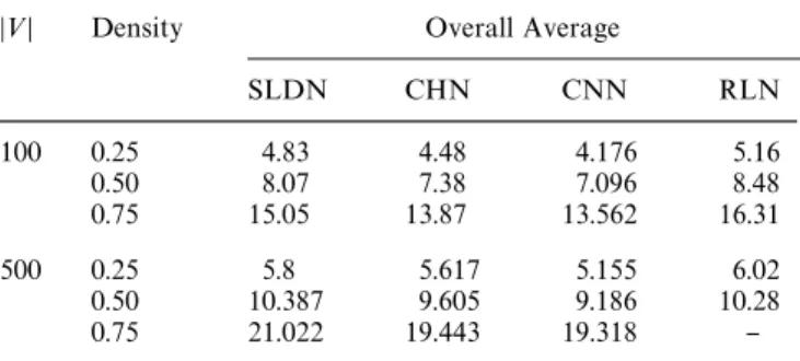
Table 1 Average Cliques Sizes found for 100- and 500-graphs with density of 0.25, 0.50 and 0.75
D<D Density Overall Average
SLDN CHN CNN RLN 100 0.25 4.83 4.48 4.176 5.16 0.50 8.07 7.38 7.096 8.48 0.75 15.05 13.87 13.562 16.31 500 0.25 5.8 5.617 5.155 6.02 0.50 10.387 9.605 9.186 10.28 0.75 21.022 19.443 19.318 }
asymptotically stable equilibrium point to which all tra-jectories starting at points in its vicinity constrained in [0, 1]n converge, corresponds to a continuous isolated local minimum point of E(x). It is proved in Pekergin et al. (1998) for E(x) with the considered A that: 1) Any stable equilibrium point is also asymptotically stable, equiva-lently any local minimum point must be isolated. 2) The asymptotical equilibria necessarily occur on vertices of the hypercube [0, 1]n. 3) The continuous local minima co-incide with the discrete local minima of E(x) under the hypercube constraint [0, 1]n. 4) Any converged vertex is actually a maximal clique. 5) For almost all initial states in the hypercube, any trajectory goes to one of the vertices corresponding to maximal clique. In other words, only the trajectories starting exactly on nonstable equilibria, which is known to be a zero measure, do not give a maximal clique. Therefore, calculating the steady-state solutions of the di!erential equation system 4 with E(x)"
xTA1x!eTx is equivalent to "nding maximal cliques of
a graph given with the adjacency matrix A.
4 Simulation results
Performance of di!erent clique "nding methods are com-pared in Table 1 for random graphs of di!erent vertex size and densities for SLDN, CHN, CNN, RLN. Average maximum cliques where the averages are taken over the test graphs generated with the same characteristics, i.e. the
vertex size and densities, are considered as a primary performance measure. Another performance measure is also considered, in which the averages are computed for the same test set but taking into account only the best results obtained on each graph is 5 and 10 independent runs with random initial conditions. This measure shows the ability of the methods to "nd di!erent search direc-tions when it is started from a di!erent initial point. The results are summarized in Table 2. Since the RLN always starts with the same initial states, results for this method are not included.
5 Conclusion
The maximum clique problem which is an NP-hard dis-crete optimization problem is reviewed here. Some basic formulations and methods used in solving this problem have been summarized, especially with emphasize on con-tinuous methods. The main contribution of this work is given in Sect. 3. In this section, gradient and quasi-gradi-ent systems were discussed, and it is shown that, even a system which has discontinuous right-hand side and hence can not be classi"ed as both of these, a discussion similar to the above mentioned systems' optimizing dy-namics can still be made. This discussion is carried on for a recently proposed dynamic optimizer, namely the saturated linear dynamical network, and to show gradient like (more precisely, completely stable) dynamics of such systems. La Salle's invariance principle is extended to the systems with a discontinuous right-hand side. Simulation results for continuous methods, namely the SLDN, CHN, CNN and RLN are given. It is concluded that gradient-like dynamical systems as continuous solution methods can be applied to the quadratic formulation of the max-imum clique problem, o!ering good approximations.
References
Chiang HD, Chu CC (1996) A systematic search method for obtain-ing multiple local optimal solutions of nonlinear programmobtain-ing problems. IEEE Trans CASI 43, 2: 99}109
Chua LO, Yang Y (1988) Cellular neural networks: theory. IEEE Trans Circuits Syst 35: 1257}1272
Chua LO, Wang NN (1978) Complete stability of autonomous reciprocal nonlinear networks. Int J Circuit Theory and Appli-cations. 6: 211}241
Crescenzi P, Fiorini C, Silvestri R (1991) A note on the approxima-tion of the max-clique problem. Inf Proc Lett. 40 1: 1}5 Funabihi N, Takefuji Y, Lee KC (1992) A neural network model for
"nding a near maximum clique. Parallel and Distributed Comp 14: 340}344
Garey MR, Johnson DS (1979) Computers and intractibility: a guide to the theory of NP-completeness. Freeman, New York
Grosberg S (1976) Adaptive pattern classi"cation and universal recording. Biolog Cybernetics 23: 121}134 and 187}202 Grossmann Y (1995) Applying the INN model to the max clique
problem. Second DIMACS Implementation Challenge, DIMACS series in Discrete Math and Theoretical Comp Science, American Math Society, Rhode Island
Hirsch MW, Smale S (1974) Di!erential equations. Dynamical sys-tems and linear algebra. Academic Press, New York
Hop"eld JJ (1982) Neural networks and physical systems with emergent collective computational abilities. Proc Math Acad Sci 79: 2554}2558
Hou L, Michel AN (1998) Asimptotic stability of systems with saturation constraints. IEEE Trans Automatic Control 43, 8: 1148}1154
Jagota A (1994) A Hop"eld style network with graph theoretic characterization. J Artf Neur Net 1: 145}167
Jagota A (1995) Approximating maximum clique with a Hop"eld network. IEEE Trans Neur. Net 6, 3: 724}735
La Salle (1968) Stability theory for ordinary di!erential equations. J. Di!erential Equations 4: 57}65
Luenberger DG (1973) Introduction to linear and nonlinear pro-gramming. Addison-Wesley, California
Motzkin TS, Straus EG (1965) Maxima for graphs and new proof of a theorem of turan. Canada J Math 17: 533}540
Pardolas PM, Phillips AT (1990) A global optimization approach for solving the maximum clique problem. Int J Comp Math 133: 209}216
Pardalos PM, Rodgers GP (1992) A branch and bound algorithm for the maximum clique problem. Comp Ops Res 19 5: 363}375 Pardolas P, Xue J (1994) The maximum clique problem. J Global
Optim 4: 301}328
Pekergin F, MorguKl OG and GuKzelis, C (1998) A saturated linear dynamical net work for approximating maximum clique. IEEE Trans on CAS I (in press)
Pelilo M (1995) Relaxation labeling networks for the maximum clique problem. J Artf Neur Net 2, 4: 313}328
S,engoKr NS, Yalimn ME, hakmr Y, UGier M, GuKzelis, C, Pekergin F, MorguKl OG (1998) Solving maximum clique problem by cellular neural network. Electronics Letters 34, 15: 1504}1506
Vidyasagar M (1978) Nonlinear systems analysis. Prentice Hall, New Jersey
View publication stats View publication stats