A GENETIC ALGORITHM-BASED SEARCH FOR PARAMETRIC REFORM ALTERNATIVES FOR THE TURKISH PENSION SYSTEM: 2005-2060
The Institute of Economics and Social Sciences of
Bilkent University
by
MUSTAFA ARTUN ALPARSLAN
In Partial Fulfillment of the Requirements for the Degree of MASTER OF ARTS
in
THE DEPARTMENT OF ECONOMICS BILKENT UNIVERSITY
ANKARA
I certify that I have read this thesis and have found that it is fully adequate, in scope and in quality, as a thesis for the degree of Master of Arts in Economics.
Assoc. Prof. Serdar Sayan Supervisor
I certify that I have read this thesis and have found that it is fully adequate, in scope and in quality, as a thesis for the degree of Master of Arts in Economics.
Prof. Gönül Turhan-Sayan Examining Committee Member
I certify that I have read this thesis and have found that it is fully adequate, in scope and in quality, as a thesis for the degree of Master of Arts in Economics.
Asst. Prof. Ümit Özlale
Examining Committee Member
Approval of the Institute of Economics and Social Sciences
Prof. Erdal Erel Director
iii
ABSTRACT
A GENETIC ALGORITHM-BASED SEARCH FOR PARAMETRIC REFORM ALTERNATIVES FOR THE TURKISH PENSION SYSTEM: 2005-2060
Alparslan, Mustafa Artun M.A., Department of Economics Supervisor: Assoc. Prof. Serdar Sayan
August 2005
In this thesis, we search for parametric reform alternatives so as to achieve a balance in the long term accumulated difference between pension expenditures and revenues of the SSI, the largest pension fund in Turkey, from 2005 to 2060. The projected worker-retiree composition of the pension system is allowed to change along with proposed policy changes in contribution and replacement rates. These changes in population structure are modeled by estimated work and pension income elasticities of labor supply values so that the resulting changes in the incomes of the worker could now affect the retirement decision. Possible policy alternatives are then found by a genetic algorithm developed for this purpose. Finally, the results obtained from the program are compared with previous and current reform proposals.
ÖZET
TÜRK EMEKLİLİK SİSTEMİ İÇİN PARAMETRİK REFORM
ALTERNATİFLERİNİN GENETİK ALGORİTMA YARDIMIYLA SAPTANMASI: 2005-2060
Alparslan, Mustafa Artun Yüksek Lisans, İktisat Bölümü Tez Yöneticisi: Doç. Dr. Serdar Sayan
Ağustos 2005
Bu tezde, Türk emeklilik sisteminin 2005-2060 yılları arasındaki uzun vadeli gelir gider dengesini sağlayabilecek parametrik reform alternatifleri aranmaktadır. Çalışmada, öncekilerden farklı olarak SSK’ya tabi nüfusun uzun dönem tahmini çalışan-emekli bileşiminde bağlama ve prim oranlarında yapılacak ayarlamaları takiben gözlenecek değişiklikler gözönüne alınmaktadır. Bu değişiklikler, çalışan ve emekli maaşlarındaki hareketlerin işgücü yapısı üzerindeki etkilerini tahmin etmeyi kolaylaştıran, esneklik tahminleri kullanılarak modellenmektedir. Bu çerçevede muhtemel politika alternatifleri bu amaçla geliştirilen bir genetik algoritma yardımıyla saptanmaktadır. Elde edilen sonuçlar şu anda gündemde olan ya da yakın geçmişte uygulanmış reform alternatifleriyle karşılaştırılmaktadır.
TABLE OF CONTENTS
ABSTRACT... iii
ÖZET ... iv
TABLE OF CONTENTS... v
LIST OF TABLES... vi
LIST OF FIGURES ... vii
CHAPTER 1 ... 1
CHAPTER 2 ... 8
CHAPTER 3 ... 20
3.1 The Objective Function... 20
3.2. The Constraints ... 25
3.2.a Retirement Age Constraint ... 26
3.2.b Work and Pension Income Elasticities of Labor Supply Constraints30 CHAPTER 4 ... 38
4.1 Scenario 1... 39
4.2 Scenario 2... 44
4.3 Elasticity Sensitivity Analysis for Scenarios ... 49
CHAPTER 5 ... 52
SELECT BIBLIOGRAPHY ... 54
APPENDIX... 56
A.1 The Main GA Program (mainga) ... 56
LIST OF TABLES
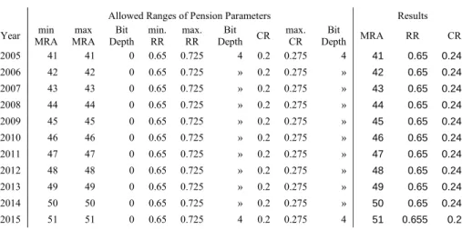
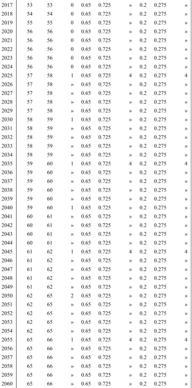
Table 1: Parametric Adjustments in 1999, 2002, and 2006 (Expected) ... 38 Table 2: Policy Proposal and the GA Output for Scenario 1... 40 Table 3: Allowed Ranges and the GA Output for Scenario 1... 45
LIST OF FIGURES
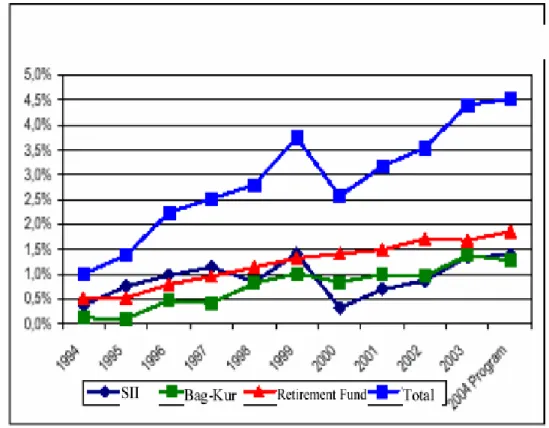
Figure 1: Transfers to Social Security Institutions by the Treasury ... 4
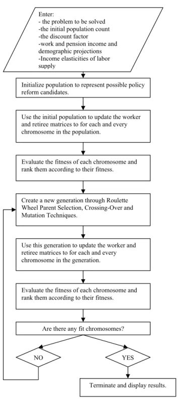
Figure 2: Flowchart for the Main Genetic Algorithm... 13
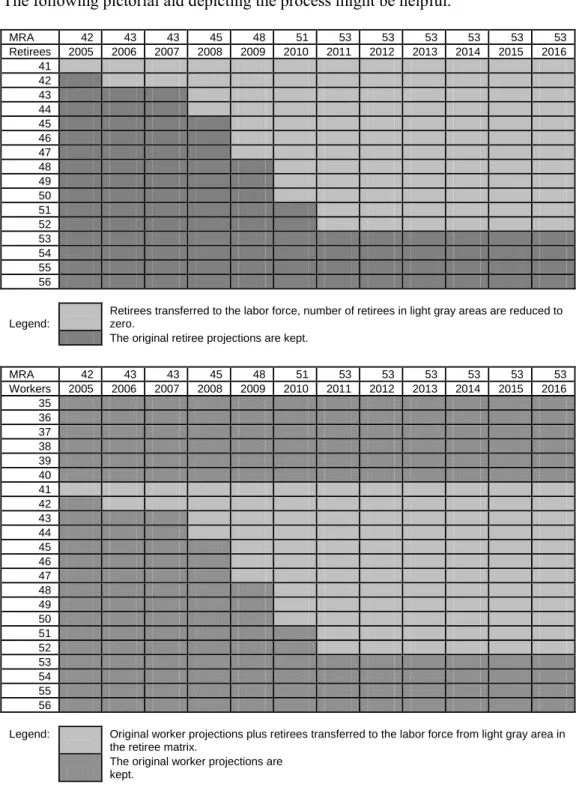
Figure 3: Retirement Age Constraint Pictorial Aid ... 28
Figure 4: Retirement Age Constraint Implementation Algorithm... 29
Figure 5: Elasticity Constraints Implementation Algorithm... 36
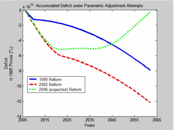
Figure 6: Accumulated Deficit under Parametric Adjustment attempts... 39
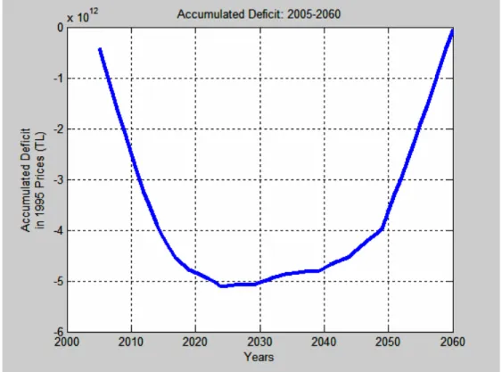
Figure 7: Accumulated Deficit for Scenario 1... 42
Figure 8: Yearly Surplus and Deficit for Scenario 1 ... 43
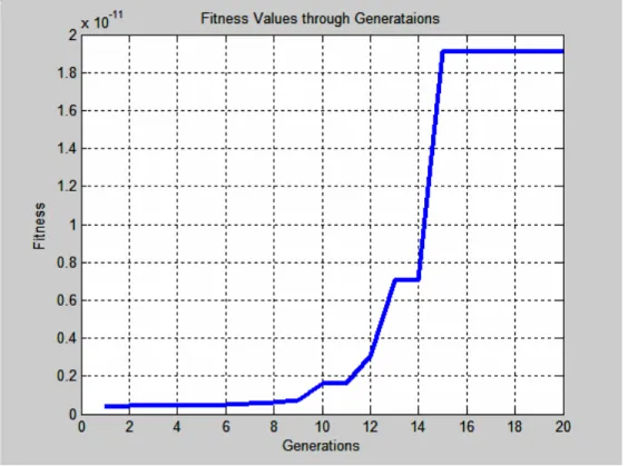
Figure 9: Fitness Values through Generations in Scenario 1... 44
Figure 10: Accumulated Deficit for Scenario 2... 46
Figure 11: Original and Policy Induced Workforce Projections ... 47
Figure 12: Yearly Surplus and Deficit for Scenario 2 ... 48
Figure 13: Fitness Values through Generations in Scenario 2... 49
Figure 14: Elasticity Sensitivity Analysis for Scenario 1 ... 50
CHAPTER 1
INTRODUCTION
The reason of existence for any government is to provide its citizens with some basic services such as security, justice, and education. In this framework, a social security system plays an important role by letting elderly citizens maintain at least a minimum living standard after they become unable to pay for their consumption with their labor.
A common approach to help retired workers pay for their own consumption is to operate a pension system which collects premiums from the current worker’s paychecks to finance the elderly workers through a distribution system. The system is called Pay-As-You-Go (PAYG) to accentuate the re-distribution aspect.
The PAYG systems were first established in the second half of the 19th
century to fund the current retirees with contributions out of current worker’s income while promising the current workers the same treatment when they have reached their old age. The high ratio of workers to retirees at the time of their establishment enabled PAYG systems to run surpluses for several decades, despite generous retirement benefits they provided. In Europe, the baby-boomers of the 1940s and 1950s helped maintain these high worker retiree ratios, keeping the PAYG systems running without incurring deficits. Yet, increasing life-expectancies caused the number of retirees to increase and decreasing fertility
rates slowed down the growth in the number of workers in many countries leading to pensions crises. It became obvious in many OECD countries, for example, that the fast-graying population cannot be funded by the current workers without initiating serious policy changes (Kenc and Sayan 2001a).
In one of the early contributions recognizing the problem, Auerbach et. al. (1989) studied four OECD countries using an OLG model and warned against the dangers of declining worker to retiree ratios ahead. Likewise, Chand and Jaeger (1996) noted the importance of the implications of aging in a society from the point of view of pension systems, and discussed how balances could be controlled by changes in the fundamental parameters of the system: the rate of contributions out of workers’ wages (contribution rate), the rate of work time average of wages replaced by pension income (replacement rate), and the minimum retirement age. Chand and Jaeger (1996) concluded by pointing to the need to create a fully-funded, defined contribution scheme within or outside the existing PAYG systems, since the PAYG system balances would continue to deteriorate unless necessary steps are taken to ensure a smooth transition to accommodate the requirements of the demographic developments ahead to remedy the system.
The establishment of PAYG pension funds in Turkey followed the same natural path in the aftermath of World War 2 through the creation of three different pension funds: Emekli Sandığı (ES), Sosyal Sigortalar Kurumu (SSK), and Esnaf ve Sanatkarlar ve Diğer Bağımsız Çalışanlar Sigorta Kurumu (BAĞ-KUR), for three different types of workers: public sector employees, private sector employees, and self-employed craftsmen and artisans, respectively. The ratio of workers to retirees remained high in the following decades until the 1980s. In fact, this ratio was expected to stay high enough not to cause concern at
least until the 2020s because of the high fertility rates in Turkey. Thus, unlike its counterparts in other OECD countries the Turkish pension system could be run without the need for drastic changes in pension parameters. Nevertheless, pension balances in Turkey quickly deteriorated starting from the 1990s due to the shortsighted and populist interventions by the policy makers (TUSIAD, 2004).
A political decision in 1992 aimed to reap the benefits of popular support lowered the minimum retirement age to as low as 38 in women and 43 in men who have paid their premiums for 20 years to earn their retirement. This implied that anyone contributing to the system for 20 years could continue to receive retirement benefits for the next 35 years (MLSS/SSI, 2004). The expected effect for the government was increased popularity among the working people by retiring them from the workforce earlier than usual and transferring their old jobs to younger workers to reduce unemployment, and hence to gain more popularity. Furthermore, the amount of pension income provided to the retirees often exceeded their active working wages, increasing people’s incentive to retire early. The young retirees often continued to work in their old jobs after retirement thereby avoiding premium payments and complementing their wages with pension income. As a result, the expected employment generation effects were not observed (MLSS/SSI, 2004; Sayan, 2005). Combined with the mismanagement of accumulated funds during the early decades of the pension system, the lack of political will to stop leakages due to the number of unregistered workers, and the reluctance to punish the employers who did not pay their contribution rates on time, the pension system began to report considerable deficits after the 1990s (Sayan, 2005).
The government’s first attempt to correct this problem (via the social security reform of 1999) involved increasing the minimum retirement age to 58 for women and 60 for men after a transition period of 10 years. However, the non-linear age increasing scheme was soon ruled out by the Constitutional Court on the grounds of violating social justice. The Court required a smoother transition in increasing retirement ages and the government had to extend the transition period to 20 years while decreasing the minimum retirement age to 56 for women and 58 for men.
The following figure taken from MLSS/SSI (2004) shows the transfers made by the Treasury to social security institutions in terms of the ratio of transfers to the nation’s GDP.
The figure shows a steady increase in transfers to GDP ratio until 1999 when a major parametric reform was legislated. The decline in the SSI deficit indicates the temporary success of the 1999 act to rectify the situation. However, with the help of a ruling of the Turkish Constitutional Court, which found the 1999 act to be violating social justice, the steady increase in budgetary transfers to social security institutions could not be stopped and total social security deficit reached up to 4.5% of the GDP in 2003. The amount of transfers made to these institutions in 2004 was 5 percent of the GDP, or USD 15 billion. Furthermore, total value of transfers made to the social security system by the end of 2003 discounted at Turkish Treasury Bill interest rates translates to 345 billion New Turkish Liras, or 1.24 times the total consolidated government debt at the time (MLSS/SSI, 2004).
Having recognized the magnitude of the problem, various researchers also studied parametric reform alternatives and their consequences. Sayan and Kenc (1999) used an overlapping generations (OLG) general equilibrium model to study the effects of increasing retirement ages in Turkey. Sayan and Kiraci (2001a) and Sayan and Kiraci (2001b) investigated alternatives based on grid search techniques to find reasonable retirement age, contribution and replacement rate combinations to minimize the pension deficit over a model horizon between 1995 and 2060. These studies were significant as they were the first attempts to formally model balances of the Turkish pension system in a 66-year horizon, forward-looking framework to suggest sustainable parameter configurations. Sayan and Turhan-Sayan (2001) used a genetic algorithm approach to speed up the slow grid-search process to identify parametric reform alternatives over the 2000-2060 period. They, however, did not consider the effects of changes in
contribution and replacement rates on choices between work and retirement decisions.
An OLG model was used in TUSIAD (2004) to study the general equilibrium effects of a transition from the PAYG system to the funded system. The study showed that such a transition could boost the GDP as much as two percent per year.
The approach to be followed in this thesis is based on Sayan and Turhan-Sayan (2001). Even though the genetic algorithm developed there is very efficient, the interaction between the number of workers and retirees and changes in pension parameters could be modeled more realistically to find more relevant policy choices for the Turkish pension system.
Furthermore, Sayan and Turhan-Sayan (2001) create a model of the SSI system where optimal values of the retirement age can be searched for all years between 2000 and 2060, while the contribution and replacement rates can only be changed once and for all during the whole model horizon. Modifying the model in such a way to let all parameters be changed as frequently as a year would give a wider range of alternatives to policy makers.
The purpose of this thesis is to extend the work of Sayan and Turhan-Sayan (2001) by allowing for the projected worker-retiree composition to change along with the changes in contribution and replacement rates according to the estimated elasticity values so that the resulting changes in the incomes of the worker could now affect the retirement decision. Coupled with the possibility of yearly changes in contribution and replacement rates towards their optimal values introduced to the model here, it will become possible to observe whether the results in Sayan and Turhan-Sayan (2001) can be improved upon.
The organization of the thesis is as follows. The next chapter provides a brief introduction to the genetic algorithms. Chapter 3 describes the model used, while the associated results are presented in Chapter 4. Finally, Chapter 5 concludes the discussion.
CHAPTER 2
GENETIC ALGORITHMS
A genetic algorithm (GA) is a set of instructions that try to maximize or minimize an objective function by mimicking the survival-of-the-fittest mechanism of the nature as described in the Darwinian theory of evolution. To illustrate the idea, let us consider reproduction of a species. A population of species creates a pool of offspring, each born carrying a combination of the hereditary content of both of its parents. The offspring is then released into the nature. An offspring with a high quality genetic inheritance can adapt quickly to the nature and has a higher chance of survival and reproduction than others with a lower quality genetic inheritance. The offspring with higher quality genetic material eventually reach the reproduction stage where they mate with other high-quality genetic material offspring to produce more offspring that are even better equipped to survive. Certain mutations along the way could further enhance the survival chances of upcoming parents and hence their offspring. Thus, the survival-of-the-fittest mechanism explains how genetic material improves to make the population better suited to their surroundings with the passage of each generation.
The use of this idea in solving an optimization problem was first suggested by John Holland in the early 1960s (Holland, 1992). To see how he has transformed the elements of the theory of natural selection as the building blocks
of a computer algorithm, one must first introduce basic concepts of the natural selection process.
Genes are the most crucial element distinguishing an individual from others and the sole constructs that carry information about an individual’s inherited characteristics. They are basically certain molecules (bases) lined up on a long molecule-chain called the DNA. In nature, a DNA strand contains four different bases adenine, thymine, guanine and cytosine (abbreviated A, T, G, and C respectively). The line-up of these bases contains instruction codes for every chemical process in the cell, defining the fitness of the cell in nature. Shortly, genes in biology represent a string that carries an individual’s unique properties for nature’s processing. Such a string of length n, where n is a natural number, contains 4
n different combinations of line-up and carries immense possibilities for
biological diversity.
Even though combining four different symbols to construct a string is also possible in computer science, it is generally easier to construct a string made up 0’s and 1’s (called a binary string or a chromosome) due to the binary nature of computation theory. This is a very useful concept since the bit-strings formed to represent the genetic inheritance properties of the cell can now be easily evaluated by a fitness function. A binary bit string A is formally represented as
N n
A∈{0,1}n, ∈ , e.g.
A 6 bit binary string → 0 1 0 0 1 0
Corresponding to sexual reproduction in nature is a biological term, cross-over. Crossing over is the creation of new genetic content from two parents by means of a random exchange of the corresponding parts of the DNA strands. Crossing over process promotes diversity in the nature and helps produce new
generations capable of adapting to nature. This process has its counterpart in a GA which works through the exchange of the bits indexed before the cross-over point with each other while keeping the chromosome order. The process yields two new chromosomes. The cross-over operation can be formally described by letting
n
B
A, ∈{0,1} be the binary strings and c∈{1,...,n−1}be the randomly chosen
cross-over point. Now, let any binary string A be divided into two binary strings
−
c
A and A where c+ A represents the binary string formed by the first c bits of A. c− Naturally, Ac+ represents the rest of A. Then, the functional form becomes:
( , , ) ( , ), , c c, c c
CrossOver A B c = C D where C =A B D− + =B A− + A 6 bit Crossing-Over Example where c=3:
A 1 0 1 0 0 0 B 0 1 0 1 0 1
C 1 0 1 1 0 1 D 0 1 0 0 0 0
The nature’s role in this process is twofold. First of all, it decides on the offspring’s genetic content quality. In a GA, this role is captured by assigning a fitness value to the bit-strings with the help of a fitness function. Formally, a fitness function can be represented as:
ℜ ∈ ∈ →F A F A f( ) , {0,1}n,
where A is a length n binary string and F is a real number. The function f is
generally assumed to assign higher values to the fitter binary strings.
The second role of the nature is the selection of pairs for reproduction. Genetically fit individuals have a higher chance to survive. They may also have some additional characteristics that help them find mates more easily than others. Then, those positive qualities of that individual would have a higher chance of being passed on to the next generation. This is replicated in a GA by ranking the
fitness of individuals and associating a reproduction criterion to that ranking. For instance, “The Roulette Wheel Parent Selection Technique” takes the fittest (say 10) chromosomes from the population and lets them reproduce according to their fitness values. This way, each chromosome gets to reproduce with a probability
} 10 ,..., 2 , 1 { , ) ( 10 1 ∈ =
∑
= k F F R P i i kk . In cases where some of the fitness values are
negative, it is always possible to assign positive values to the fitness values by adding a positive constant to all of the fitness values. Since the value of the added constant affects the probability distributions greatly, the selection of this constant is an issue of algorithm design. If one does not want to assign probabilities, the same probability for reproduction can always be assumed for all, again say 10, fittest chromosomes.
However, in some cases the whole population might be involved in reproduction instead of the fittest, say, ten. This would decrease the best individuals’ rates of survival but increase the diversity in the population to create more potent candidates for reproduction. This is called soft selection and has been shown to outdo some hard selection algorithms in terms of more rapid rates of improvement in for some evolutionally stagnant populations. Galar (1989) shows that soft selection methods proved to be more efficient than hard ones in crossing Gaussian multimodal regions. This is a result of the adaptability that the least fit individuals might bring into the system.
Another important factor in natural selection process is mutations. Mutations are changes in the gene-content of the offspring independent of the crossing-over process. When applied to GA’s mutations are random one or possibly more bit changes in the chromosome. With some preassigned
probability, a zero at a particular location in the bit-string of an offspring may be changed to one or a one may be changed to zero.
Based on the terminology introduced, the algorithm can be verbally described as follows. After binary strings and the fitness functions are designed, an initial population is created randomly. That population is then evaluated by the fitness function. At the next stage, the population creates a new generation by means of crossing-over and mutation. This population too is ranked according to the fitness value. If a preset fitness criterion is satisfied by any of the chromosomes, the algorithm stops. If not, a new population is initiated from the existing one.
A flowchart for the algorithm is given in the next page in Figure 2.
A simple optimization task can be designed to demonstrate the use of genetic algorithms. Consider a simple optimization problem such as a finding the nearest point to the zero of a cubic function defined over a given interval.
Assume that the algorithm searches for the point which makes the value of the curve ( ) ( 4)3
f x = x− closest to zero. Naturally, the desired point for this curve is attained at x= and the desired value is 0. Now, let the search be in the region 4
[0, 7.5]
x∈ . This means that the chromosomes making up the population should be designed so that their range is x∈[0, 7.5]. Now, define a 4-bit chromosome in this range such that every chromosome represents a different point in the
[0, 7.5]
x∈ region to represent the whole population of possible solutions. Thus the solution is said to have a 4-bit depth in the desired solution domain. Furthermore, imposing a linear distribution of points in the domain might be desirable and convenient. Then, a function g(A), which has a 4-bit binary string or equivalently a four-digit number in modulo 2 as domain, maps A∈{0,1}4 to its
Figure 2: Flowchart for the Main Genetic Algorithm Enter:
- the problem to be solved -the initial population count -the discount factor
-work and pension income and demographic projections -Income elasticities of labor supply
Initialize population to represent possible policy reform candidates.
Use the initial population to update the worker and retiree matrices to for each and every chromosome in the population.
Evaluate the fitness of each chromosome and rank them according to their fitness.
Create a new generation through Roulette Wheel Parent Selection, Crossing-Over and Mutation Techniques.
Use this generation to update the worker and retiree matrices to for each and every chromosome in the generation.
Are there any fit chromosomes?
NO YES
Evaluate the fitness of each chromosome and rank them according to their fitness.
relative range value, x∈[0,7.5]. Here ( ) 0 1mod ( )2 2
g A = + A , where 0 is the
starting point of the fitness function’s search range (x∈[0, 7.5]), 1
2 is the step size between each element in the search range, and mod ( )2 A represents the
possible values that any chromosome might take. Note that the minimal and maximal domain values for the fitness functions are achieved at A=0000 and
1111 A= , respectively. 0 1 2 3 2 mod (0000) 0 2 0 2 0 2 0 2 0 (0000) 0 0 2 2 2 g = + = ⋅ + ⋅ + ⋅ + ⋅ = = 0 1 2 3 2 mod (1111) 1 2 1 2 1 2 1 2 15 (1111) 0 7.5 2 2 2 g = + = ⋅ + ⋅ + ⋅ + ⋅ = =
The fitness of each chromosome should increase in proportion with its closeness to zero. Assigning the fitness function below to the chromosomes fulfills this requirement.
3 3 2 1 1 1 ( ) mod ( ) | ( ( )) | 2 | ( ( ) 4) | 2 | ( 4) | 2 2 F A A f g A g A = = = + − + − +
where the constant 2 is added to the denominator of the function,F A( ), to avoid any possible zeros in the denominator.
Now, the population is initiated with four chromosomes chosen randomly from the whole population of 24 =16. Then, the respective reproduction
probability for a four-chromosome initial population is
10 1 ( ) ( ) , {1, 2,3, 4} ( ) k k i i F A P A k F A = = ∈
∑
Let these initial chromosomes, their associated fitness and their reproduction probabilities be given as
1 1 1 1 1 1 1 1 1 1 1 1 2 2 2 2 1 1 1 1 3 3 3 3 1 1 1 4 4 4 1100 ( ) 6.0 ( ) 0.1000 ( ) 0.0808 0111 ( ) 3.5 ( ) 0.4760 ( ) 0.3804 1010 ( ) 5.0 ( ) 0.3333 ( ) 0.2694 0110 ( ) 3.0 ( ) 0.3333 A g A F A P A A g A F A P A A g A F A P A A g A F A P = ⎯⎯→ = ⎯⎯→ = ⎯⎯→ = = ⎯⎯→ = ⎯⎯→ = ⎯⎯→ = = ⎯⎯→ = ⎯⎯→ = ⎯⎯→ = = ⎯⎯→ = ⎯⎯→ = ⎯⎯→ 1 4 (A ) 0.2694= As seen from the above results, the fittest chromosome is the 2nd one since it
has the highest probability of passing on to the next generation. These probability values are then used to create the next generation by “The Roulette Wheel Parent Selection Technique”. Assume that after the necessary random number generations, the following chromosomes were attached to each other in the following cross-over places.
2 1 1 1 3 1 2 1 1 2 4 2 2 1 1 3 2 3 2 1 1 4 3 4 ( , ,1) 1100 ( , , 2) 0111 ( , ,1) 0010 ( , ,3) 1010 A CrossOver A A A CrossOver A A A CrossOver A A A CrossOver A A = = = = = = = =
The second generation’s fitness values are reported below.
2 2 2 2 1 1 1 1 2 2 2 2 2 2 2 2 2 2 2 2 3 3 3 3 2 2 2 4 4 4 1100 ( ) 6.0 ( ) 0.1000 ( ) 0.0807 0111 ( ) 3.5 ( ) 0.4760 ( ) 0.3800 0010 ( ) 1.0 ( ) 0.0345 ( ) 0.2701 1010 ( ) 5.0 ( ) 0.3333 A g A F A P A A g A F A P A A g A F A P A A g A F A P = ⎯⎯→ = ⎯⎯→ = ⎯⎯→ = = ⎯⎯→ = ⎯⎯→ = ⎯⎯→ = = ⎯⎯→ = ⎯⎯→ = ⎯⎯→ = = ⎯⎯→ = ⎯⎯→ = ⎯⎯→ 2 4 (A ) 0.2691= The third generation is reproduced by the same process.
3 2 2 1 4 2 3 2 2 2 2 4 3 2 2 3 1 4 3 2 2 4 2 1 ( , ,1) 1111 ( , , 2) 0110 ( , ,3) 1100 ( , , 2) 0100 A CrossOver A A A CrossOver A A A CrossOver A A A CrossOver A A = = = = = = = =
3 3 3 3 1 1 1 1 3 3 3 3 2 2 2 2 3 3 3 3 3 3 3 3 3 3 3 4 4 4 1111 ( ) 7.5 ( ) 0.0223 ( ) 0.0233 0110 ( ) 3.0 ( ) 0.3333 ( ) 0.3488 1100 ( ) 6.0 ( ) 0.1000 ( ) 0.1046 0100 ( ) 4.0 ( ) 0.5000 A g A F A P A A g A F A P A A g A F A P A A g A F A P = ⎯⎯→ = ⎯⎯→ = ⎯⎯→ = = ⎯⎯→ = ⎯⎯→ = ⎯⎯→ = = ⎯⎯→ = ⎯⎯→ = ⎯⎯→ = = ⎯⎯→ = ⎯⎯→ = ⎯⎯→ 3 4 (A ) 0.5232= The fourth generation is reproduced by the same process.
4 3 3 1 4 3 4 3 3 2 4 4 4 3 3 3 3 2 4 3 3 4 3 3 ( , , 2) 0100 ( , ,3) 0100 ( , , 2) 1110 ( , , 2) 1100 A CrossOver A A A CrossOver A A A CrossOver A A A CrossOver A A = = = = = = = =
The corresponding fitness values and reproduction probabilities are:
4 4 4 4 1 1 1 1 4 4 4 4 2 2 2 2 4 4 4 4 3 3 3 3 4 4 4 4 4 4 0100 ( ) 4.0 ( ) 0.5000 ( ) 0.4407 0100 ( ) 4.0 ( ) 0.5000 ( ) 0.4407 1110 ( ) 7.0 ( ) 0.0345 ( ) 0.0304 1100 ( ) 6.0 ( ) 0.1000 A g A F A P A A g A F A P A A g A F A P A A g A F A P = ⎯⎯→ = ⎯⎯→ = ⎯⎯→ = = ⎯⎯→ = ⎯⎯→ = ⎯⎯→ = = ⎯⎯→ = ⎯⎯→ = ⎯⎯→ = = ⎯⎯→ = ⎯⎯→ = ⎯⎯→ 4 4 (A ) 0.0881= After reaching this point, the algorithm could be stopped since the optimum value obtained in future generations will, most probably, be unchanged due to the high reproduction probability of the fittest chromosome yielding x= . Then 4 there should not be any reasons to continue the search. However, as opposed to this steady state, there might be some points in the algorithm where the search is stuck at some not very desirable value. Then, mutations can be initiated into the system to avoid these problems.
It should be noted, that as stated by one of the pioneers of evolutionary algorithms, Fogel (1999), GA’s possess further capabilities to solve much more complex problems than the one above. He asserts that the ease of their implementation and the broad range of areas where they are applicable are very valuable characteristics for those who work with very unusual functional forms. Usual methods of optimization used in economics generally require functions of
continuous, differentiable and, even, convex nature in order to serve their purpose properly. However, there are classes of problems which none of these conditions might hold. The objective function might be discrete and moreover it might have local extrema, rendering some gradient based solutions infeasible. Non-linear constraints and non-stationary conditions in real world problems also increase computational burden making it difficult to use some of the conventional techniques. Genetic algorithms are thus useful in solving complex optimization problems with such characteristics without necessitating simplifying assumptions about functional forms.
A GA model is particularly suitable for the problem in this thesis since the objective function is discrete and the feasible region is not easy to visualize. Still, it is certain that there is some kind of monotonic behavior expected of the objective function in response to increases or decreases in pension parameter values. So, even though numerous local maxima and minima may be encountered, GA developed here must be capable of handling them.
With its ease of application to economics problems, and its robustness with discrete functions, the GA’s have become a useful tool for economists. The pioneering work in the field is done by Arifovic (1994) where she simulates learning in a rational expectations equilibrium model. In the model, competitive firms use a genetic algorithm to update their decision on which and what amount of good to use the next period in a one good production economy.
In another paper, Arifovic (1995) presents a two-period overlapping generations (OLG) model with money, low inflation and seignorage to show that the individuals’ policies dictated by learning through GA are the same as the ones at unique monetary steady state equilibrium. Bullard and Duffy (1998) extend
this model to a multi-period OLG model to find out a high inflation equilibrium, a low inflation equilibrium as well as undecided cases. Another application of GA’s in economics is the game theoretical solution search where a game is modeled as a GA and the possible equilibria are searched for. An example to this application is Özyıldırım (1997). The paper approximates solutions to linear non-quadratic open loop Nash-Cournot equilibrium, where agents involved in a multi-period game creating their own policies about what to do at the beginning of each period at time 0 without cooperating with each other. Once the policy is made in time 0, the agents stick to their decisions and the game is played accordingly. The result is the case where none of the agents can deviate from the equilibrium policy without getting worse off. For a two-person game, the solution starts out by creating a GA structure for each player. Each GA structure has the player’s utility function, and population. At the beginning, each player sends out a random strategy to the other player, which the other player accepts as the best response to his action. With the best response at hand, players then move on to create new strategies from the acquired best response functions and their previous moves. The process works as the initial population is ranked with the help of the evaluation function and cross-overs and mutations are performed in the selected group. At the end of the selection process, a new strategy is formed and sent to the other player, initiating the next round. The algorithm terminates once the termination criteria are satisfied.
In another study, Alemdar and Özyıldırım (1998) use GA’s to search for optimal policies in a North/South trading game.
Another interesting use to GA’s in economics/finance can be found in Chen and Yeh (2002) who use GA’s to model agents in a stock market setting through
an “agent-based economics” approach which uses GA’s heavily to simulate a real life situation.
CHAPTER 3
THE MODEL
3.1 The Objective Function
The current Turkish pension system is run on a pay-as-you-go basis which finances the payments made to current pensioners through contributions collected from current workers. The Social Security Institution therefore needs to bring present value of its future receipts as close to the present value of its commitments as possible to run the system without significant deficit or surplus.
In the model, the time horizon is taken to be the period between years 2005 and 2060, when Turkey’s population is expected to have stabilized and reached its steady state at less than 100 million people. Thus, the payments-receipts balance achieved by 2060 will represent a reasonable approximation to the SSI’s deficit level for 2061 and onwards.
One way of restoring the long-term actuarial balance of the SSI is to minimize the following expression, mostly adapted from Sayan and Turhan-Sayan (2001). 0 2005 2060 , , , , , , 2005 1 ( , , ) ( , , ) 1 s.t.
min
t t t le mwa t a t a t t a t a t RR CR A t a A a a RR rw R RR CR A CR rw W RR CR A δ − = = = = ⎡ ⎤ ⎛ ⎞ − ⎢ ⎥ ⎜ + ⎟ ⎝ ⎠ ⎣ ⎦∑
∑
∑
(1)Retirement Age Constraints: : 41 t, : 2005 2060 : a a A t t ∀ ≤ < ∀ ≤ ≤ , , , ( o, o, ) ( o, o, o) ( o, o, o) (2) a t a t a t W RR CR A = W RR CR A +R RR CR A , ( o, o, ) 0 (3) a t R RR CR A = : 75 t, : 2005 2060 : a a A t t ∀ ≥ ≥ ∀ ≤ ≤ , , ( o, o, ) ( o, o, o) (4) a t a t W RR CR A = W RR CR A , , ( o, o ) ( o, o, o) (5) a t a t R RR CR A =R RR CR A
Income Elasticity of Labor and Pension Constraints:
Constraints for policy change in the initial year of the model:
: t , : 2005 2060 a A a mwa t t ∀ ≤ < ∀ ≤ ≤ ' 2005 ' 2060 2005 2060 , ' ' 2005 ' ' 2006 2005 2006 ({ } ,{ o} ,{ } ,{ o} , ) a t W RRτ ττ== RRτ ττ== CRτ ττ== CRτ ττ== A = , ( , , ) , ( , , ) (6) o o o o a t a t W RR CR A +DW RR CR A ' 2005 ' 2060 2005 2060 , ' ' 2005 ' ' 2006 2005 2006 R ({ } ,{ o} ,{ } ,{ o} , ) a t RR RR CR CR A τ τ τ τ τ τ== τ τ== τ τ== τ τ== = , , R ( o, o, ) ( o, o, ) (7) a t RR CR A −DWa t RR CR A
Constraints for policy change for years 2006 through 2059:
: t , , : 2005 2060, : 2006 2060 a A a mwa t τ t t τ τ ∀ ≤ < ∀ < ≤ ≤ ∀ ≤ ≤ ' ' 2060 ' ' 2060 , ({ '}' 2005,{ '} ' 1 ,{ }' 2005,{ }' 1 , ) o o a t W RRτ ττ τ== RRτ τ ττ == + CRτ ττ τ== CRτ τ ττ== + A = ' 1 ' 2060 ' 1 ' 2060 , ' ' 2005 ' ' ' 2005 ' ({ } ,{ o} ,{ } ,{ o} , ) (8) a t W RRτ ττ τ== − RRτ τ ττ== CRτ ττ τ= −= CRτ τ ττ== A ' ' 2060 ' ' 2060 , ' ' 2005 ' ' 1 ' 2005 ' 1 R ({ } ,{ o} ,{ } ,{ o} , ) a t RR RR CR CR A τ τ τ τ τ τ τ τ== τ τ τ== + τ τ== τ τ τ== + =
' 1 ' 2060 ' 1 ' 2060 , ' ' 2005 ' ' ' 2005 ' R ({ } ,{ o} ,{ } ,{ o} , ) (9) a t RR RR CR CR A τ τ τ τ τ τ τ τ= −= τ τ τ== τ τ= −= τ τ τ== : t , , : 2005 2060, : 2006 2060 a A a mwa t τ t t τ τ ∀ ≤ < ∀ ≥ ≤ ≤ ∀ ≤ ≤ ' ' 2060 ' ' 2060 , ({ '}' 2005,{ '} ' 1 ,{ }' 2005,{ }' 1 , ) o o a t W RRτ ττ τ== RRτ τ ττ == + CRτ ττ τ== CRτ τ ττ== + A = ' 1 ' 2060 ' 1 ' 2060 , ' ' 2005 ' ' ' 2005 ' ({ } ,{ o} ,{ } ,{ o} , ) a t W RRτ ττ τ== − RRτ τ ττ== CRτ ττ τ= −= CRτ τ ττ== A + ' 1 ' 2060 ' 1 ' 2060 , ' ' 2005 ' ' ' 2005 ' ({ } ,{ o} ,{ } ,{ o} , ) (10) a t DW RRτ ττ τ== − RRτ τ ττ== CRτ ττ τ= −= CRτ τ ττ== A ' ' 2060 ' ' 2060 , ' ' 2005 ' ' 1 ' 2005 ' 1 R ({ } ,{ o} ,{ } ,{ o} , ) a t RR RR CR CR A τ τ τ τ τ τ τ τ== τ τ τ== + τ τ== τ τ τ== + = ' 1 ' 2060 ' 1 ' 2060 , ' ' 2005 ' ' ' 2005 ' R ({ } ,{ o} ,{ } ,{ o} , ) a t RR RR CR CR A τ τ τ τ τ τ τ τ= −= τ τ τ== τ τ= −= τ τ τ== − ' 1 ' 2060 ' 1 ' 2060 , ' ' 2005 ' ' ' 2005 ' ({ } ,{ o} ,{ } ,{ o} , ) (11) a t DW RRτ ττ τ== − RRτ τ ττ== CRτ ττ τ= −= CRτ τ ττ== A
Constraints for the final year of the model:
: t , , : 2005 2059 a A a mwa t τ t t ∀ ≤ < ∀ < ≤ ≤ , Wa t(RR CR A, , )= ' 2059 ' 2060 ' 2059 ' 2060 , ({ '}' 2005,{ o'} ' 2060,{ }' 2005,{ o} ' 2060, ) (12) a t W RRτ ττ== RRτ ττ== CRτ ττ== CRτ ττ== A , ( , , ) a t R RR CR A = ' 2059 ' 2060 ' 2059 ' 2060 , ({ '} ' 2005,{ o'}' 2060,{ } ' 2005,{ o} ' 2060, ) (13) a t R RRτ ττ== RRτ ττ== CRτ ττ== CRτ ττ== A : t , 2060 a A a mwa t ∀ ≤ < = , Wa t(RR CR A, , )= ' 2059 ' 2060 ' 2059 ' 2060 , ({ '}' 2005,{ '} ' 2060,{ }' 2005,{ } ' 2060, ) o o a t W RRτ ττ== RRτ ττ== CRτ ττ== CRτ ττ == A − ' 2059 ' 2060 ' 2059 ' 2060 , ' ' 2005 ' ' 2060 ' 2005 ' 2060 ({ } ,{ o} ,{ } ,{ o} , ) (14) a t DW RRτ ττ== RRτ ττ== CRτ ττ== CRτ ττ== A , R (a t RR CR A, , )= ' 2059 ' 2060 ' 2059 ' 2060 , ' ' 2005 ' ' 2060 ' 2005 ' 2060 R ({ } ,{ o} ,{ } ,{ o} , ) a t RR RR CR CR A τ τ τ τ τ τ== τ τ== τ τ== τ τ== −
' 2059 ' 2060 ' 2059 ' 2060 , ' ' 2005 ' ' 2060 ' 2005 ' 2060 ({ } ,{ o} ,{ } ,{ o} , ) (15) a t DW RRτ ττ== RRτ ττ== CRτ ττ== CRτ ττ == A and , , , , , ( ) ( ) ( ) ( ) 1 1 , if 0 ( ) 2 1 2 1 0 , else a t t a t t a t t a t t a t t t t t W dCR R dRR W dCR R dRR DW λ CR λ RR λ CR λ RR ⎧ ⎡ ⋅ ⋅ ⎤ ⎡ ⋅ ⋅ ⎤ − + − + < ⎪ ⎢ ⎥ ⎢ ⎥ ⋅ =⎨ ⎣ − ⎦ ⎣ − ⎦ ⎪ ⎩ (16) where t
CR : Average contribution rate per worker in year t (0<CRt <1),
t
RR : Average replacement rate of a pensioner in year t to replace average work income (0<RRt <1)
t
A : Minimum retirement age in year t (At <mwa),
, ,
RR CR A : {RRt t}t==20602005,{CRt t}t==20052060,{ }At tt==20052060
,
/ a t( , , )
W R RR CR A : Projected number of workers/pensioners of age a in year t as a function of pension parameters in the policy matrix, {RR CR A, , },
,
/ ( o, o, o)
a t
W R RR CR A : Original projection of number of
workers/pensioners of age a in year t as a function of pre-1999 pension parameters, { o, o, o}
RR CR A ,
,
/ ( o, o, )
a t
W R RR CR A : Projection of number of workers/pensioners of age a in year t updated according to the new value of A only,
' ' 2060 ' ' 2060
, ({ '}' 2005,{ '} ' 1 ,{ }' 2005,{ }' 1 , )
o o
a t
W RRτ ττ τ== RRτ τ ττ== + CRτ ττ τ== CRτ τ ττ== + A : A worker
population matrix showing the steps in transforming the final form of retirement age constraint, , ( o, o, )
a t
W RR CR A , to the final elasticity constrained worker matrix, Wa t, (RR CR A, , ), where τ represents the year up to which the transformation has successfully been completed.
,
a t
rw : Average real work income of pensioners of age a in year t ,
t a
rw, : Average real work income of workers of age a in year t ,
0
a :Minimum working age, le :Life expectancy.
λ :Income elasticity constant, ρ : Pension elasticity constant, mwa : Maximum working age, δ : Discount factor,
The objective function to be minimized describes the difference between the total present discounted values of contribution receipts and pension payments to face the SSI over the model horizon, provided that pension parameters are { o, o, o}
RR CR A . Total wages earned by the workers covered by the SSI in a given year t is calculated by multiplying the number of workers in a given cohort,
, ( , , )
a t
W RR CR A , by the average wage of workers belonging to that cohort, rwa t, , and then summing the result over all age groups in year t,
, , ( , , ) le a t a t a mwa rw W RR CR A =
∑
. Total contribution revenue of the SSI for a given year t is calculated by multiplying this sum with the contribution rate for that year, CR . t The resulting value is converted to the present value terms by a standard presentvalue operator to yield,
0 2005 , , 1 ( , , ) 1 t mwa t a t a t a a CR rw W RR CR A δ − = ⎛ ⎞ ⎜ + ⎟
⎝ ⎠
∑
. Then, the presentvalues are summed over for all possible years, to obtain total present value of the
future receipts of the SSI,
0 2005 2060 , , 2005 1 ( , , ) 1 t t mwa t a t a t t a a CR rw W RR CR A δ − = = = ⎛ ⎞ ⎜ + ⎟ ⎝ ⎠
∑
∑
Total present value of the future pension expenditure of the SSI is obtained
in a similar way resulting in
2005 2060 , , 2005 1 ( , , ) 1 t t t le t a t a t t a A RR rw R RR CR A δ − = = = ⎛ ⎞ ⎜ + ⎟ ⎝ ⎠
∑
∑
.Therefore, subtracting the expenditures from revenues, we get the present value of the total deficit/surplus. Normally, a publicly managed pension fund would not aim at high surpluses but would ideally avoid high deficits. Naturally, the deficit/surplus value should be as close to zero as possible. This is achieved in the model by using the absolute value operator whose global minimum is naturally zero.
3.2. The Constraints
The optimization discussed up to this point requires an extensive knowledge of the labor force covered by SSI, which is represented by the following data:
i. The projections of the number of workers, , ( o, o, o)
a t
W RR CR A , for each age a ( where a takes integer values 15 through 75 plus) and for each year t (where t takes integer values 2005 through 2060),
ii. The projections of the number of retirees, Ra t, (RR CR Ao, o, o), for
each age a ( where a takes integer values 41 through 80 plus) and for each year t (where t takes integer values 2005 through 2060),
iii. The projections of the average annual real work incomes of workers, rw , for each age a ( where a takes integer values 15 through 75 a t, plus) and for each year t (where t takes integer values 2005 through 2060),
iv. The projections of the average annual real work incomes of retirees, rw , for each cohort a ( where a takes integer values 41 through a t,
80 plus) for each year t (where t takes integer values 2005 through 2060), where the plus sign following an integer represents the set of all integers after that integer.
Initially, four projection matrices, ,( o, o, o)
a t
W RR CR A , Ra t, (RR CRo, o,Ao),
,
a t
rw , and rwa t o, , , for items (a) through (d) above are available through ILO
(1996) and Sayan and Turhan-Sayan (2001). These matrices contain projections that are based on pre-1999 values of pension parameters. Therefore, they include non-zero values for the number of retirees for all years in the model for ages as low as 38.
The results of our optimization exercises therefore rely heavily on these projections but the projected values of gross real wages will assume not to be affected by the changes brought forth by alternative reform parameters.
Such dependence creates the need to update the original projections on the numbers of workers and retirees accordingly with the changes in pension parameters. This is achieved by using the retirement age and elasticity constraints.
3.2.a Retirement Age Constraint
The first step in updating projections based on the pre-1999 values of pension parameters is the creation of worker/retiree projections in accordance with the proposed increases in retirement ages, A. The retirement age vector A is designed such that its first element corresponds to the proposed minimum retirement age in year 2005, and its second element corresponds to the retirement
age in year 2006. Proceeding like this, the last element of the vector would be matched with the last year in the model horizon, 2060.
The elements of this vector take monotonically increasing values since it is assumed that age is increased from one year to another, it will not be reduced ever again in the future. This is a reasonable assumption since the life expectancy of the population is also expected to increase in the future.
The algorithm starts out from year 2005 which is the first element in A. The retirement age is checked and found to be, say, a . This means that the retirees 1 who are below age a in 2005 will no longer be able to retire as dictated in the 1 original retiree matrix and will have to work until the newly posted retirement age. These people are consequently transferred to the labor force, W, increasing the number of workers at age a1in year 2005 by the number of retirees at age a1in
the same year. Naturally, this brings down the number of retirees at that age in that year strictly to zero. The new labor force values after a proposed 2005 retirement age policy change are presented below.
: 41 t, : 2005 2060 : a a A t t ∀ ≤ < ∀ ≤ ≤ , , , ( o, o, ) ( o, o, o) ( o, o, o) (17) a t a t a t W RR CR A = W RR CR A +R RR CR A , ( o, o, ) 0 (18) a t R RR CR A = : 75 t, : 2005 2060 : a a A t t ∀ ≥ ≥ ∀ ≤ ≤ , , ( o, o, ) ( o, o, o) (19) a t a t W RR CR A = W RR CR A , , ( o, o, ) R ( o, o, o) (20) a t a t R RR CR A = RR CR A
Repeating the same steps for retirement ages for years 2006 to 2060 yields the new worker and retiree projections, , ( o, o, )
a t
W RR CR A and , ( o, o, ) a t
R RR CR A . The following pictorial aid depicting the process might be helpful.
MRA 42 43 43 45 48 51 53 53 53 53 53 53 Retirees 2005 2006 2007 2008 2009 2010 2011 2012 2013 2014 2015 2016 41 42 43 44 45 46 47 48 49 50 51 52 53 54 55 56 Legend:
Retirees transferred to the labor force, number of retirees in light gray areas are reduced to zero.
The original retiree projections are kept.
MRA 42 43 43 45 48 51 53 53 53 53 53 53 Workers 2005 2006 2007 2008 2009 2010 2011 2012 2013 2014 2015 2016 35 36 37 38 39 40 41 42 43 44 45 46 47 48 49 50 51 52 53 54 55 56 Legend:
Original worker projections plus retirees transferred to the labor force from light gray area in the retiree matrix.
The original worker projections are kept.
Furthermore, a flowchart sketching the algorithm is shown below.
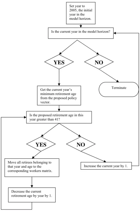
Figure 4: Retirement Age Constraint Implementation Algorithm
The matrices updated to take the retirement age constraint into account are used in calculating the additional changes to result from changes in CR and RR.
Is the current year in the model horizon?
YES
NO
Is the proposed retirement age in this year greater than 41?
YES
NO
Increase the current year by 1. Move all retirees belonging to
that year and age to the corresponding workers matrix.
Decrease the current retirement age by year by 1.
Terminate Set year to
2005, the initial year in the model horizon.
Get the current year’s minimum retirement age from the proposed policy vector.
3.2.b Work and Pension Income Elasticities of Labor Supply
Constraints
In the model, the disposable income of a worker is calculated by multiplying the real annual wage income of the worker by (1-CR), the percentage of income received by the worker net of contributions paid to the SSI. That is
,
(1 t) a t I = −CR rw .
Similarly, the pension income is calculated by multiplying the average real annual wage income of the pensioner over the working period by RR, the replacement rate: P=RR rwt a t, .
In the light of these definitions, we can consider the response of individuals who are between the statutory entitlement age and maximum working age to changes in CR and/or RR. Since these individuals have the option of continuing to work or taking their retirement depending upon the incentives, changes in CR and RR would affect the worker-retiree composition of this age group.
Now, let λ be the income elasticity of labor supply. Then,
, , , , ( ) ( ) (21) a t a t a t a t dW W dWI WI λ ⋅ ⋅ =
where work income is WIa t, = −(1 CR rwt) a t, and At ≤ ≤a mwa. Naturally,
0
λ> , and its definition can be rearranged to yield , ,
, , ( ) ( ) a t a t a t a t dW W dWI λ WI ⋅ ⋅ = . Note that , , , , ( ) ( ) a t a t t a t t a t dW dW dCR dWI dCR dWI ⋅ ⋅ ≡
, , ( ) a t t a t t dW dCR dWI dCR ⋅ ≡ , , ( ) a t t (22) a t dW dCR rw ⋅ ≡ −
Combining this with (21), we can write
, , , , , ( ) ( ) ( ) (23) (1 ) a t a t a t a t t a t t dW W rw W dCR λ WI λ CR ⋅ ⋅ ⋅ = − = − − , ( ) , ( ) (24) (1 ) a t a t t t dW W dCR CR λ ⋅ ⋅ = = − −
Equation 24 enabled us to convert income elasticity of labor supply into a contribution rate elasticity. This equation could alternatively be written as
, 1 , 1 , ( ) ( ) (25) ( ) (1 ) a t a t t t a t t W W CR CR W λ CR + ⋅ − ⋅ = − + − ⋅ −
with discrete changes in percentage terms on both sides, allowing us to interpret λ as net wage elasticity of labor supply. Corresponding to λ is an RR elasticity that allows us to capture the response of individuals aged a at time t to changes in RR. Let this elasticity be denoted by ρ and defined as
, , , , ( ) ( ) (26) a t a t a t a t dR R dPI PI ρ ⋅ ⋅ =
where PIt =RR rwt a t, and ρ >0. Then,
, , , , , , ( ) (27) ( ) a t a t a t t a t a t a t t dR dPI dRR rw R ρ PI ρ RR rw ⋅ = = ⋅
Thus, ρshows the percentage change in the number of retiree resulting from a one percent increase in the replacement rate. Equation 27 can be equivalently written as , 1 , 1 , ( ) ( ) (28) ( ) (1 ) a t a t t t a t t R R RR RR R ρ RR + ⋅ − ⋅ = − + − ⋅ −
Now, remembering that the population, p , for any particular year and age is a t, constant regardless of the policy changes, Ra t, ( )⋅ +Wa t, ( )⋅ =pa t,
, ( ) , , ( ) (29) a t a t a t t t t dW dp dR dRR dRR dRR ⋅ ⋅ = −
Since p is constant, we can write the following by keeping Equation 27 in a t, mind. , ( ) , ( ) a t a t t t dW dR dRR dRR ⋅ ⋅ = − , ( ) a t (30) t R RR ρ ⋅ = −
Equation 24 and Equation 30 together imply
, , , ( ) ( ) 2 ( ) 1 a t t a t t a t t t W dCR R dRR dW CR RR λ ⋅ ρ ⋅ ⎡ ⎤ ⋅ = −⎢ + ⎥ − ⎣ ⎦ or , , , ( ) ( ) 1 ( ) (31) 2 1 a t t a t t a t t t W dCR R dRR dW CR RR λ ⋅ ρ ⋅ ⎡ ⎤ ⋅ = − ⎢ + ⎥ − ⎣ ⎦
in which dWa t, may be positive or negative depending on the magnitudes of changes in CR and RR.
However, it should be noted that the changes that demand an increase in the number of workers (such as a reduction in CR) while keeping the registered population constant cannot be met. This is because the retirees who by definition have quit contributing to the system cannot be returned to the workforce. Then, increasing the number of workers without reducing the number of retirees would require increasing the projected number of people within the age group under consideration. Hence, we assume that transfers from projected workforce matrices to the projected retiree matrices are unidirectional in the sense that only workers can be transferred to the retiree matrices. Then, the change in the number of workers for any change in CR and RR would be
, , , ( ) , if ( ) 0 ( ) (32) 0 , else a t a t a t dW dW DW ⋅ = ⎨⎧ ⋅ ⋅ < ⎩
Projected numbers of workers and retirees are updated in response to changes in CR and RR as follows:
Initially, the worker and retiree projections that are based on the current values of contribution and replacement rates are manipulated to address minimum retirement age changes. From now on, the resulting matrices will be referred to as
, ( o, o, )
a t
W RR CR A and , ( o, o, ) a t
R RR CR A , where the replacement of A by A o
indicates that minimum retirement age modification is already completed on the matrix, whereas keeping o
RR and CRo indicates that no modifications on account
of changes in CR and RR have been introduced to matrices yet.
Once a change is introduced to the contribution and replacement rates in the first year of the model, 2005, the worker retiree matrices must be adjusted so as to obtain new matrices based on the new contribution and replacement rates for the year 2005. That is, ({ }τ' 2005= ,{ o}τ' 2060= ,{ }τ' 2005= ,{ o}τ' 2060= , )and
' 2005 ' 2060 ' 2005 ' 2060
, ({ '} ' 2005,{ '}' 2006,{ }' 2005,{ }' 2006, )
o o
a t
R RRτ ττ== RRτ ττ== CRτ ττ== CRτ ττ== A . This is achieved by applying the elasticity formula above to transfer some of the workers projected to stay in the workforce under old values of CR and RR to the projected retiree population for all of the remaining years in the model. After making the necessary worker transfers, the transferred workers are subtracted from the retiree matrix to keep the population constant.
: t , : 2005 2060 a A a mwa t t ∀ ≤ < ∀ ≤ ≤ ' 2005 ' 2060 2005 2060 , ' ' 2005 ' ' 2006 2005 2006 ({ } ,{ o} ,{ } ,{ o} , ) a t W RRτ ττ== RRτ ττ== CRτ ττ== CRτ ττ== A = , , W ( o, o, ) ( o, o, ) (33) a t RR CR A +DWa t RR CR A ' 2005 ' 2060 2005 2060 , ' ' 2005 ' ' 2006 2005 2006 R ({ } ,{ o} ,{ } ,{ o} , ) a t RR RR CR CR A τ τ τ τ τ τ== τ τ== τ τ== τ τ== = , , R ( o, o, ) ( o, o, ) (34) a t RR CR A +DWa t RR CR A
As a consequence, the change injected into the worker retiree projections becomes a once-and-for-all change affecting all present and future numbers of retirees.
Once the data is updated like this, the next year’s projections,
' 2006 ' 2060 2006 2060 , ({ '} ' 2005,{ '}' 2007,{ } 2005,{ } 2007, ) o o a t R RRτ ττ== RRτ ττ== CRτ ττ== CRτ ττ== A and ' 2006 ' 2060 2006 2060 , ({ '}' 2005,{ o'} ' 2007,{ } 2005,{ o} 2007, ) a t
W RRτ ττ== RRτ ττ== CRτ ττ== CRτ ττ== A , will be created similarly whenever there is a change in the policy. In general, for an arbitrary year τ in the horizon, in the case of a policy change, relevant projections are updated as follows. First of all, the process starts out by noting that current and future policies cannot affect the number of workers and retirees projected for the previous years. Hence, these values become natural elements of current matrices. Then, the change in current policy variables is applied to every age group in every
year for the remaining years in the horizon to update the matrices in accordance with the policy changes. The algorithm thus moves forward to cover all years in the model horizon. A general approach is presented below.
: t , , : 2005 2060, : 2006 2060 a A a mwa t τ t t τ τ ∀ ≤ < ∀ < ≤ ≤ ∀ ≤ ≤ ' ' 2060 ' ' 2060 , ({ '}' 2005,{ '} ' 1 ,{ } ' 2005,{ }' 1 , ) o o a t W RRτ ττ τ== RRτ τ ττ == + CRτ ττ τ== CRτ τ ττ== + A = ' 1 ' 2060 ' 1 ' 2060 , ' ' 2005 ' ' ' 2005 ' ({ } ,{ o} ,{ } ,{ o} , ) (35) a t W RRτ ττ τ== − RRτ τ ττ== CRτ ττ τ= −= CRτ τ ττ== A : t , , : 2005 2060, : 2006 2060 a A a mwa t τ t t τ τ ∀ ≤ < ∀ ≥ ≤ ≤ ∀ ≤ ≤ ' ' 2060 ' ' 2060 , ({ '}' 2005,{ '} ' 1 ,{ }' 2005,{ }' 1 , ) o o a t W RRτ ττ τ== RRτ τ ττ== + CRτ ττ τ== CRτ τ ττ== + A = ' 1 ' 2060 ' 1 ' 2060 , ' ' 2005 ' ' ' 2005 ' ({ } ,{ o} ,{ } ,{ o} , ) a t W RRτ ττ τ== − RRτ τ ττ== CRτ ττ τ= −= CRτ τ ττ == A + ' 1 ' 2060 ' 1 ' 2060 , ' ' 2005 ' ' ' 2005 ' ({ } ,{ o} ,{ } ,{ o} , ) (36) a t DW RRτ ττ τ== − RRτ τ ττ== CRτ ττ τ= −= CRτ τ ττ == A : t , , : 2005 2060, : 2006 2060 a A a mwa t τ t t τ τ ∀ ≤ < ∀ < ≤ ≤ ∀ ≤ ≤ ' ' 2060 ' ' 2060 , ' ' 2005 ' ' 1 ' 2005 ' 1 R ({ } ,{ o} ,{ } ,{ o} , ) a t RR RR CR CR A τ τ τ τ τ τ τ τ== τ τ τ== + τ τ== τ τ τ== + = ' 1 ' 2060 ' 1 ' 2060 , ' ' 2005 ' ' ' 2005 ' R ({ } ,{ o} ,{ } ,{ o} , ) (37) a t RR RR CR CR A τ τ τ τ τ τ τ τ= −= τ τ τ== τ τ= −= τ τ τ== : t , , : 2005 2060, : 2006 2060 a A a mwa t τ t t τ τ ∀ ≤ < ∀ ≥ ≤ ≤ ∀ ≤ ≤ ' ' 2060 ' ' 2060 , ({ '} ' 2005,{ '} ' 1 ,{ } ' 2005,{ } ' 1 , ) o o a t R RRτ ττ τ== RRτ τ ττ== + CRτ ττ τ== CRτ τ ττ == + A = ' 1 ' 2060 ' 1 ' 2060 , ' ' 2005 ' ' ' 2005 ' R ({ } ,{ o} ,{ } ,{ o} , ) a t RR RR CR CR A τ τ τ τ τ τ τ τ= −= τ τ τ== τ τ= −= τ τ τ== − ' 1 ' 2060 ' 1 ' 2060 , ' ' 2005 ' ' ' 2005 ' ({ } ,{ o} ,{ } ,{ o} , ) (38) a t DW RRτ ττ τ== − RRτ τ ττ== CRτ ττ τ= −= CRτ τ ττ == A
The data for the final year of the model horizon can also be calculated from the previous year’s data in a similar way.
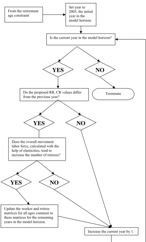
Figure 5: Elasticity Constraints Implementation Algorithm Is the current year in the model horizon?
YES
NO
Do the proposed RR, CR values differ from the previous year?
YES
NO
Increase the current year by 1. Does the overall movement
labor force, calculated with the help of elasticities, tend to increase the number of retirees?
YES
Update the worker and retiree matrices for all ages common to these matrices for the remaining years in the model horizon.
Terminate Set year to
2005, the initial year in the model horizon. From the retirement
age constraint
The program that translates the effects of changes in the minimum retirement age and contribution/replacement rates into the model becomes a part of the fitness calculating code to order the chromosomes according to their usefulness.