A network science approach to correlations between course achievement and community structure in school friendship networks

(1)

KADIR HAS UNIVERSITY

GRADUATE SCHOOL OF SCIENCE AND ENGINEERING

A Network Science Approach to

Correlations Between Course

Achievement and Community Structure

in School Friendship Networks

Kenan Kafkas

Supervisor: Assoc Prof. Mehmet Nafiz Aydın

Advisor: Asst. Prof. Nazım Ziya Perdahçı

This dissertation is submitted for the degree of

Master of Management Information Systems

(2)

(3)

Declaration

”I, Kenan Kafkas, confirm that the work presented in this thesis is my own. Where information has been derived from other sources, I confirm that this has been indicated in the thesis”.

Kenan Kafkas January 2017

(4)

Acknowledgements

I would like to thank the department of Management Information Systems in the faculty of Engineering and Natural Sciences at Kadir Has University for providing me this precious studying opportunity. I gratefully thank my academic advisor Dr. Mehmet Nafiz Aydın and co-advisor Dr. Nazım Ziya Perdahçı and also Dr. Ahmet Salih Biçakcı for their consistent support in my studies and research. They always did their best to provide help and encouragement. I also would like to thank fellow students in the MIS department for their helpful discussions.

(5)

(6)

Abstract

In this research we examine a secondary school social network. We apply social network analysis (SNA) techniques on the close friendship structure of the students. Our aim is to answer the following questions regarding the network. The first question is, what are the mixing values with respect to test achievement scores, gender and class. The second question is, how are the communities in the network structured. Such findings can be significant assets in understanding and improving the learning environment. They may be used to help teachers and school managers in deciding more workable and efficient student matchings. For this study, we conducted a survey to a group of 10th grade students and gathered the necessary information to construct the social network around the school. Our findings show that the friendship in overall network is neither assortative nor disassortative with respect to academic success, in other words the two attributes are not correlated. On the other hand, gender and class mixing measures are significantly high which not surprisingly suggests that the students prefer to bond with their classmates and also with the same gender friends. Finally, after examining the communities within each classroom, we observe similar community structures. In the light of these findings we propose a method for composing the classrooms to construct an efficient and successful learning environment.

(7)

List of figures

3.1 A simple network model showing nodes and links. . . 10

4.1 Graph of the SFN. Colors represent classes, the size indicates GPA. Commu-nities are grouped in the layout. . . 16

4.2 Graph of the SFN. Colors represent gender, size indicates GPA . . . 17

4.3 Histogram of Random Network Clustering Coefficients. . . 18

4.4 Histogram of Diameters of random graphs. . . 18

4.5 Average clustering coefficient of random networks (blue) over a range of wiring probability p. Average distances (red). Horizontal lines indicate clustering coefficient of SFN (purple) and average distance of SFN (orange). 19 4.6 Degree distributions of random Barabasi-Albert graph. . . 20

4.7 Degree distribution of SFN . . . 20

4.8 Number of communities in random graph models . . . 21

4.9 Sub-graphs of each class. Colors represent communities, size indicates GPA 23 4.10 Graph of overall SFN. Nodes marked in circles show isolated groups. . . . 25

4.11 A part of overall SFN. Green node between green and orange classes has a high betweenness centrality. . . 26

(11)

List of tables

3.1 Sample spreadsheet showing node attributes and closest friends. . . 9

3.2 Node list with three attributes . . . 9

3.3 Edge List . . . 9

4.1 Summary of the SFN characteristics . . . 15

4.2 Comparison between random graph models and SFN. . . 19

4.3 Assortativity coefficient based on academic achievement, gender and class. 22 4.4 Number of communities and assortativity coefficients within classes. . . 22

(12)

Nomenclature

Acronyms / Abbreviations

CC Clustering Coefficient

DDDM Data Driven Decision Making

GPA Grade Point Average

SFN Student Friendship Network

(13)

Chapter 1 Introduction

Social networks appear in different spots of our life. Clubs, Hospitals, Schools are presenting great opportunities to researchers to observe the social networks. Observing social structure of student networks in schools promises interesting and worthwhile results. Those results may help improve efficiency in education.

Composition of classes is one of the main issues in school management. The composition and the formation of classes play a crucial role in creating an efficient and successful classroom setting [1]. Although there has been substantial research on class formation and composition[2][3][1], there is little research focusing on network of friendship relations [4][5]. The common use of data in Data Driven Decision Making (DDDM) processes is mostly focused on achievement test scores [6]. This research aims to put an effort to add student social structure data to DDDM process.

Analyzing the friendship networks brings following questions to mind: What are the factors that play role on forming the friendships among students? What are the mixing structures in school networks? What type of communities do they form? Do classes have similar community structures? Answers of these questions may provide significant benefits for education managers, teachers and hopefully students.

In this research we explore a friendship network of a group of students. Following a survey which asks students their best friends, we cover all steps in a typical data analytic cycle from data collection to visualization, analytics and interpretation. We use Social Network Analysis (SNA) tools to examine the properties of the network. Our preferences for data cleaning and manipulation is Pandas which is a data analysis library of Python language.

(14)

2 Introduction

Gephi is the visualization software of our choice. Furthermore, for calculating network characteristics and implementing various algorithms we use igraph, which is a Network analysis library of R language.

Random networks are used in network science for several purposes. In this study we generate random graphs to test our network characteristics to see if they act randomly. In other words, we compared the observed network with random graphs to search non-random mechanisms acting inside.

We investigate the mixing behaviors in class to find correlations between course achieve-ment and the close friendship. Furthermore, we look at the number of communities not only in overall network, but also within subnetworks. In the light of the findings, we propose a method that can be utilized as an additional tool in decision making process for school managers and teachers.

1.1 Motivation and Challenges

Social network analysis studies have advanced in last 15 years. Having access to powerful analysis tools enabled researchers investigate different networks that appear in many fields. With the advance of SNA its examples in education emerged. Some researches used SNA findings to improve teaching practices, others used it to increase participation.

Understanding student networks in terms of mixing behaviors and community structures has a potential to present workable matches in student groupings. Finding methods to achieve this goal may have certain obstacles. Obtaining sufficient sample data might be difficult. We have to test our method to improve it further, however, having required authority in teaching environment might be difficult.

1.2 Summary of Contributions

(15)

1.3 Structure of the Thesis 3

• Presenting an overview of the network science and its implications on education.

• Investigating the correlation between student social relations and their academic achievement.

• Proposing a method for class composition depending on community structures.

1.3 Structure of the Thesis

The organizational structure of this thesis is as follows: Chapter 2 presents research back-ground information, and definitions on network science topics and its relevant implications in education science. Chapter 3 describes methods utilized in this study, furthermore, explains how and why the network metrics are used. Chapter 4 presents the findings and discussions. The last chapter contains the conclusion.

(16)

Chapter 2 Research Background

2.1 Network Science

The history of network science has roots going back to 18th century [7]. Euler, a Swiss mathematician was the first scientist to use the graph theory to solve the famous “Bridges of Königsberg” problem [8]. Until 1950s, the graph theory remained in the backseat of mathematics. A Hungarian mathematician Pál Erd˝os brought the graph theory to main stage with his study on random graphs [9]. Following that, in 1960s and 70s social scientists started to use graph theory to model the humans in groups. In this period, an American social psychologist Stanley Milgram introduced the small world network notion. This phenomenon captured interest of many scientists. It was interesting to see that individuals could reach one another with only few intermediaries in large human networks [8]. Another concept called betweenness centrality emerged in the same period. It is now playing important role in identifying high traffic nodes on the Internet [7].

Towards the end of the 20th century, Internet revolution caused a leap in the network science studies. In the past scientists lacked the tools to map large networks. Emergence of Internet brought numerous advantages including, development in computer technology, cheap digital storage, new methods to keep and process data. All these improvements helped researchers tackle the problem of analyzing real networks [7].

Networks appear in almost every branch of sciences. Many studies in modern scientific interest areas involve complex systems.The interactions among millions of cells or genes

(17)

2.1 Network Science 5

in biology, multitude of transactions in finance world, interaction of particles in physics, are in the domain of complex systems. All the components in these systems are highly interconnected. Because of their interlinked structure, a failure in one of these points can cause a substantial portion of the system to collapse. A small change can initiate a serious shift in collective behavior of the system. Scientists from different disciplines are visualizing and analyzing in order to understand the mechanisms working within these networks.

2.1.1 Networks

A network consists of two types of simple components, nodes and links. Nodes may represent an individual in a social network or an enzyme in a cell. The connections between nodes are called the links. They may represent kinship between individuals in social network or chemical interaction between enzymes in a cell. The term graph, refers to mathematical representation of a network. It is analogous to a wiring diagram. The terms network, node and link are mostly used for referring real world complex systems whereas the terms graph, vertices and edges are used when referring to a mathematical representation of the real world systems. These are only subtle differences and these terms are often used interchangeably [7].

A node can have more than one link. Total number of links of a node is called its degree. If links in a network has distinct direction from one node to another, this type of network is called a directed network. In an undirected network links do not have directions. There are two types of degrees in directed networks; in degree which is the number of links pointing towards a node, out degree which is the number of nodes pointing out from a node.

2.1.2 Random Networks

Random network is an artificial network which is generated by probabilistic mechanisms. Today random networks are called Erd˝os-Rényi Networks [9] referring to two Hungarian mathematicians who have great contributions to the graph theory especially, the random graph models. In a series of papers, they explained their method for creating a random graph. The steps to generate a random network is as follows. First step is creating a given number of nodes and the second step is connecting each pair of nodes only if a randomly generated number exceeds a given probability threshold. The network science uses random networks to

(18)

6 Research Background

mimic the properties of real networks. Furthermore, random networks are compared with observed networks in order to detect similarity or contrast.

2.2 Education Science

In the last decade in almost every field, data became abundant, more accessible, and more diverse. Educators quickly adapted this situation and began to involve data more often in their decision making processes. Thus, Data Driven Decision Making (DDDM) concept is introduced in education.

“DDDM in education refers to teachers, principals, and administrators systemat-ically collecting and analyzing various types of data, including input, process, outcome and satisfaction data, to guide a range of decisions to help improve the success of students and schools.” [6]

Achievement test score data is mostly used in education for DDDM. Non-achievement student outcome measures such as student attendance and graduation rates are also used in decision making [6]. However, friendship ties among students is a less studied issue in teaching environment. One of the main goals of this research is to find ways to include the data on the social structure of the school in order to broaden the abilities of DDDM. In education, schools are a way of organizing the system into functional units.

“a school is an organization engaged in a series of compositional transformations of its student population into grades, classes, and instructional groupings so that a workable match can be achieved among curriculum, instruction, and the ability of students” [1].

Establishing instructional groupings that have workable matches may be the definition of class composition. One of the useful outcomes of well-made class composition is that it enables teachers to make effective in-class groupings. Researchers have investigated various in-class grouping techniques and mentioned positive effects on achievement [10][11][12][13]. If classes are composed in an appropriate way, it is most likely that teachers can easily and accurately make grouping decisions.

(19)

2.2 Education Science 7

This is where applying SNA on friendship network may contribute substantial support to DDDM. Mapping the network visually that illustrates all the communities can help managers to establish appropriate compositions. In well-established classes forming groups can be achieved more effectively. Gathering group members from students who are more willing to collaborate with each other can result in successful education settings. One of the objectives of our study is to propose methods for composing such classes by using Social Network Analysis Tools.

(20)

Chapter 3 Methods

3.1 Data Acquisition and Preperation

The subject of this research is a student network which we refer to as Student Friendship Network (SFN). To construct its graph, we collected the data by conducting a simple survey. Since we needed to observe the friendship ties in school, we designed the survey that asks students to provide their best friends. The survey was voluntary and confidential. The students were assured that their right to privacy would be respected. To anonymize the data, we represented students with random numbers. None of the students refused to participate the study. Seven students out of 209 provided two close friends. We limited the maximum number of close friends to three to keep the data balanced. Additionally, we limited the scope of the survey to only 10th grade students. There were six 10th grade classes in the school. Students were not limited to their classes; they were free to provide their close friends across all 10th grade class.

Another type of data we collected was the course achievement data. We gathered this data from E-Okul which is an online platform of the Ministry of Education that keeps the information of all students. We used test achievement scores to calculate the course achievement data which is referred as GPA in this paper. We did not exclude any of the courses. After collecting, the data were entered in a spreadsheet. Table 3.1 shows a sample of that spreadsheet. We can see that class name, gender, GPA and the numbers representing the close friends displayed in the spreadsheet.

(21)

3.1 Data Acquisition and Preperation 9

Table 3.1 Sample spreadsheet showing node attributes and closest friends.

Id Class Name Gender GPA 1. 2. 3.

5 Class A F 71.93 23 106 54 6 Class A M 68.56 54 37 45

Both visualization tools and analysis tools require certain file formats for importing graph data. We used Gephi software for visualization and R programming language for SNA. They both accept csv file format to import graph data. We prepared two csv files that are called node list and edge list. The first one contained list of nodes along with their attributes, the second one contained list of edges that shows nodes are connected to each other. To create these files, we used Pandas which is a data analysis library for Python programming language. Table 3.2 shows sample from the node list whic has three attributes.Table 3.3 shows a portion of the edge list.

Table 3.2 Node list with three attributes

Id Class Name Gender GPA

5 10-A F 71.93 6 10-A M 68.56

Table 3.3 Edge List

Source Target 5 23 5 106 5 54 6 54 6 37 6 45

(22)

10 Methods

3.2 Network Model

In our research we modeled the Student Friendship Network in such a way that the vertices represented students. The edges between two vertices represented close friendship relation. To put it in another way, if student A claimed that student B is his or her close friend, then we connected them in the graph by an arrow pointing from node A to node B. Figure 3.1 shows the simple model of the graph. If we look at the model, we can see student A accepts student B as a close friend, student B however, does not perceive him or her as close friend. In these kind of networks edges have directions. By definition they are called directed networks. There are 209 nodes in this graph. We requested three of their best friends from the students in the survey. The resulting graph had 620 edges instead of 627 (3 * 209) due to the fact that seven of these students provided only two close friends. We did not use weighted edges which means that we did not quantify the degree of closeness of the friendship between two students.

Fig. 3.1 A simple network model showing nodes and links.

.

3.3 Small World Network

Small world network, also known as six degrees of separation, is a phenomenon which occurs when a network displays high clustering yet smaller average distance. The network of social

(23)

3.4 Network Metrics Used 11

relations among people in the world can be presented as a small world where average shortest path is calculated as 6 [14].

The classical random graph model could not produce small world networks. In a classical random graph clustering is generally lower and average distances are greater. A method for modeling Small World Networks was introduced in 1998 by Watts and Strogatz [15]. They noticed that real world networks showed high clustering coefficient yet small distances between nodes [16]. In their paper Watts and Strogatz suggested a mechanism that generates random small world graphs. In order to achieve this, the model started with given number of nodes and connected them with their given number of neighbors which forms a lattice. After that, every node is reconnected with another random node depending on a given probability which is called rewiring probability. The result is a random graph with high clustering and small average path length which are the indications of small world network. In igraph library there is a function that implements this method called watts.strogatz.game. Using this function, we generated 100 random networks for every rewiring probability in the range from %0.01 to %30. we calculated the clustering coefficient and average distance of these random graphs.

3.4 Network Metrics Used

3.4.1 Network Density

The density of a network is the ratio of total number of existing links to number of maximum possible links in the network. In other words, it shows how dense a network is relative to its maximum possible density. It is a measure that indicates the degree of connectedness of a given network. In this case study we utilized this measure in finding how the network is clustered (3.2.2) and also we used this metric to demonstrate the characteristics of the network (4.1.1).

The density of a directed network G is calculated as follows [16];

den(G) =

|E

G

|

|V

_G

|(|V

_G

|−1)

(3.1)

(24)

12 Methods

|EG| is the number of edges in the network.

|VG| is the number of vertices in the network.

3.4.2 Clustering Coefficient

The clustering coefficient of a node is the ratio of number of links between neighbors of a node and total possible number of links among neighbors. In other words, it is the degree of density that shows how much the neighbors of a given node is linked to each other [7]. This gives us local clustering coefficient (CC). For CC of a whole network we calculate the average of the CC of all nodes. For friendship networks this statistical measure has intuitive meanings: it reflects the extent to which friends of a student are also friends with each other [15].

The transitivity function in igraph calculates clustering coefficient however it is only useful for undirected graphs. Our graph is directed therefore, we use the equation specified in [17] is as follows;

cl(v) =

(A+A

T

)

3

2[d

v

(d

v

−1)−2(A

2

)]

(3.2) where:

Ais the adjacency matrix.

d_vis the total degree of vertex v which is sum of in-degree and out-degree.

The R function that applies this method [16] can be found in appendix A. We used this metric for two purposes firstly, to see whether our graph differs from random network models. Secondly, to identify if it is a small world network.

3.4.3 Assortativity

"Selective linking among vertices, according to a certain characteristic(s), is termed assor-tative mixing in the social network literature" [16]. In other words, if nodes in a network

(25)

3.4 Network Metrics Used 13

tend to link to nodes that have similar attributes with them, then we say that the network is assortative. In disassortative networks, nodes prefer to link to dissimilar nodes. For instance, marriage network is a highly disassortative network since mostly people choose to marry opposite sex. If a network is neither assortative nor disasortative then the network is called neutral. Therefore, assortative mixing or homophily property in networks shows the correlation between attributes of nodes across edges. The metric that shows assortativity is called assortativity coefficient and it is defined as follows [16];

r

_a

=

∑

i

f

ii

−∑

i

f

i+

f

+i

1−∑

i

f

i+

f

+i (3.3) where:

r_ais the assortativity coefficient. fi j is a fraction of edges in the graph that joins a vertex

in the ith category with a vertex in the jth category. f i+ is the sum ith marginal row. f +i is the sum ith marginal column.

Assortativity coefficientra(standard Pearson correlation coefficient) ranges between -1

and 1 with r = 1 indicating perfect Assortative mixing, r = 0 indicating no correlation, and r = 1 indicating perfect disassortative mixing.

We utilized assortative mixing coefficient to determine if the students have tendency to establish close friendship with similar students. We used three characteristics. The main characteristic is the test achievement score. The reason why we chose achievement scores is that this metric is widely used in Data Driven Decision Making [18]. The other characteristics are gender and class.

3.4.4 Community Detection by Modularity Analysis

Community detection is generally grouping the network in such a way that, the resulting groups have dense connections within and sparse connections between groups. In social networks communities can be any group of people that comes together for a purpose. Mem-bers of hobby clubs, families, employees in a company, they are all groups of people who are densely connected to each other. Detecting these communities may present critical information about the structure of a social network. In this research our objective is to use the community structure of the network to construct a method for class composition.

(26)

14 Methods

We used igraph library’s infomap function that implements community detection al-gorithm based on the study [19]. The corresponding R code is presented in Appendix A

(27)

Chapter 4 Findings and Discussions

4.1 Findings

This section presents a brief overview of the network structure then explains the findings of the SNA.

4.1.1 Network Characteristics

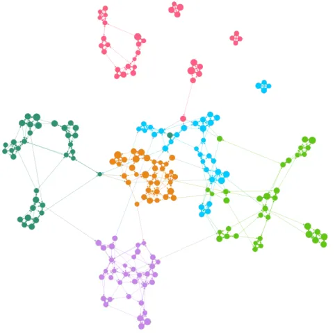
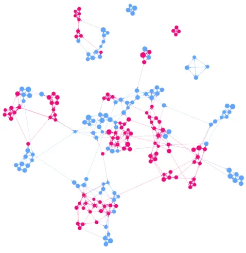
Table 4.1 demonstrates the main characteristics of the Student Friendship Network. Average degree of the network is approximately 6. This is an expected value since almost every node has 3 out-degrees. We observe quite low density of approximately 0.01 which is an expected value as well. Barabasi argues that “Real networks are sparse” [7] which fits in with our finding. Looking at the clustering coefficient we can observe a high clustering behavior which can be expected in a high school social environment. Figure 4.1 is an illustration of the network. Colors represent the six classes whereas size of the nodes represent GPA of the students. The layout of the nodes demonstrates the communities of the overall network. In figure 4.2 colors are blue and pink representing male and female students respectively.

Table 4.1 Summary of the SFN characteristics

Nodes Edges Av. Degree Density Av. Path Length Av. Clustering C. Directed

(28)

16 Findings and Discussions

Fig. 4.1 Graph of the SFN. Colors represent classes, the size indicates GPA. Communities are grouped in the layout.

(29)

4.1 Findings 17

Fig. 4.2 Graph of the SFN. Colors represent gender, size indicates GPA

4.1.2 Comparison with Random Graphs

To prove that the SFN is not random, we sampled 500 random graph models using igraph library. These random graph models had the same number of nodes and the same number of degree sequences with the SFN. Figure 4.3 shows histogram of the clustering coefficients of random graphs. In figure 4.4 we can see the histogram of diameters of random graph models. Clustering coefficient of the SFN is 0.386 whereas the random models have an average clustering coefficient of 0.021. Additionally, average network diameter of the random graph models is 9.870 whereas the diameter of the SFN is 29. These significant differences are a strong indication that our Student Friendship Network is not random.

(30)

Fig. 4.3 Histogram of Random Network Clustering Coefficients.

Fig. 4.4 Histogram of Diameters of random graphs.

4.1.3 Small World Property

In order to test if SFN shows small world behavior we need to look at the clustering coefficient and path length. And compare the results with random graph models that are generated based on a small world mechanism. After generating 100 random samples we observed that while average path length remained roughly the same, clustering was significantly higher than the clustering of the random models. This means that Student Friendship Network shows small world behavior.

(31)

4.1 Findings 19

Table 4.2 Comparison between random graph models and SFN.

Friendship Network Random Models

Clustering Coefficient 0.386 0.586

Diameter 29 25.560

Average Path Length 10.769 11.048

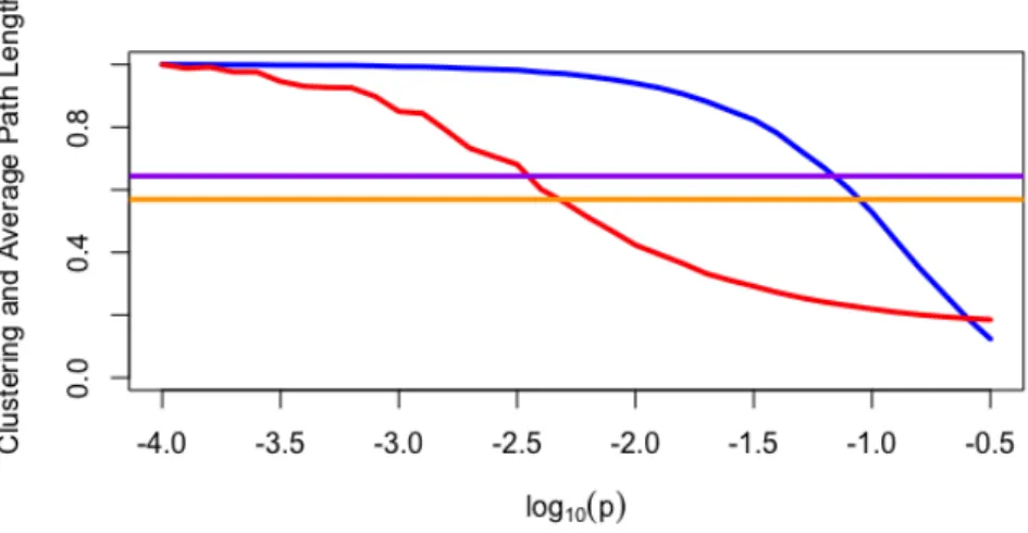
Figure 4.5 illustrates clustering coefficient (blue) and average distance (red) of random models over a range of rewiring probability p. The horizontal lines are the clustering coefficient (blue) and average distance (red) of SFN. All values are normalized for comparison purposes. We can see in the figure 4.5 that in a substantial range of p, SFN has higher clustering coefficient and smaller average distance compared to random graphs. Over this range from %7 to % 30 SFN has small network properties.

Fig. 4.5 Average clustering coefficient of random networks (blue) over a range of wiring probability p. Average distances (red). Horizontal lines indicate clustering coefficient of SFN (purple) and average distance of SFN (orange).

4.1.4 Preferential Attachment

Another type of mechanism-based random graph model is Barabasi-Albert model [20]. In this model, as the graph evolves, new nodes prefer to attach to high degree nodes. As a result of this preferential attachment degree distribution of this model tends to show a power-law

(32)

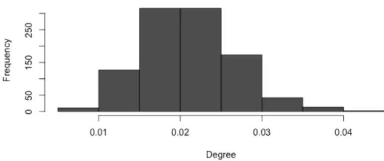
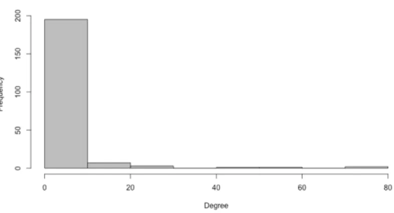
distribution [20]. Additionally, we expect fewer nodes between two vertex pairs and low clustering. In order to compare the degree distributions, we generated a random graph based on Barabasi-Albert model that has similar characteristics with our network. Then we plotted the degree distributions of both graphs. If we look at the distributions 4.7, we can see that, although distribution of the SFN is not exactly a power-law distribution it is notably close. It presents few high-degree nodes and great number of low-degree nodes. This shows that our graph has weak preferential attachment.

Fig. 4.6 Degree distributions of random Barabasi-Albert graph.

Fig. 4.7 Degree distribution of SFN

4.1.5 Number of Communities in Overall Network

The comparison between the numbers of communities in the networks can be used to assess whether there are different mechanisms working within the network. We utilized infomap

(33)

4.1 Findings 21

function of the igraph library to detect the communities in the network. It detected 35 communities. In order to test whether the fragmentation of the network is random we generated two types of random graphs. The first type was Erdos-Renyi random graph that had the same size with SFN. The second one was a random graph that had the same degree sequence. We generated 500 different realizations of each type. Figure 4.8 shows that random graphs have tendency to break into smaller number of communities, hence there are likely additional dynamics working in the SFN that are not random.

Fig. 4.8 Number of communities in random graph models

4.1.6 Assortative Mixing

Our objective is to see whether there is a correlation between friend selection and course achievement. To measure this phenomenon, we utilized assortativity coefficient of the network. In our case, we want to find out whether high GPA students tend make close friendship attachments with high GPA students and vice-versa. To assess mixing with respect to academic success, gender and class we computed assortativity coefficients respectively. Table 4.3 shows assortativity coefficients based on GPA, gender and classes. Assortativity coefficient with respect to student success is -0.004. This is strong evidence that forming of friendship does not have positive or negative correlation with course achievement. The

(34)

gender based assortativity coefficient is 0.699. This indicates that students mostly prefer same gender students as close friends. Lastly, The assortativity coefficient based on class is 0.936. As we expected this is a strong indication that sharing same classroom is an important factor in forming close friendship.

Table 4.3 Assortativity coefficient based on academic achievement, gender and class.

GPA Gender Class

Assortativity Coefficient ( r ) -0.004 0.699 0.936

4.1.7 Number of Communities within the Classes

Partitioning the network by classes produces sub-networks. Focusing on the sub-networks can be helpful to understand the structure of the classes independently. We partitioned the overall network into six sub-networks where each sub-network represents each class. Then we visualized the graphs in Gephi. The figure 4.9 shows six illustrations of each class sub-network. The colors represent the communities and the size of the nodes represent academic success based on achievement test scores.

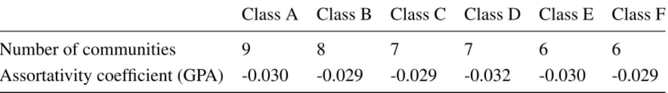
Looking at the number of communities in each class, it is approximately 7 on average and they show similar structure. The mixing behavior with respect to academic success can be observed by looking at the assortativity coefficients across classes. The values are almost the same for every class. These similarities are a good indication that there is a similar social interaction within every class. (This finding can be used to develop a method for class composition.) Although within class mixing values are similar to each other they differ from overall network assortativity. Average In-class mixing is -0.029 which demonstrates a higher degree of disassortativity relative to overall network’s mixing. This indicates that among students there is a small tendency to choose dissimilar peer. Table 4.4 shows the number of communities and the assortativity coefficients of the classes. Figures

Table 4.4 Number of communities and assortativity coefficients within classes.

Class A Class B Class C Class D Class E Class F

Number of communities 9 8 7 7 6 6

(35)

4.1 Findings 23

(a) Class A (b) Class B

(c) Class C (d) Class D

(e) Class E (f) Class F

(36)

4.2 Discussions

We have following observations based on the network analysis results. Our network is a low density network that has fair amount of clustering despite the three friend limitation. There are other limitations that need to be taken into consideration.These are mentioned in section 4.2.1.One of the key findings in this research is that achievement score based social mixing in overall network is neutral section 4.1.6. In other words, the behavior of the network in this context is not different than a random network’s behavior [16]. This result may show that in overall network students do not regard success as a positive or negative influence when it comes to bonding with peers. However, within classes we observed slight disassortativity relative to overall network value. This indicates, it is more likely that a low grade student preferred to socialize with a high grade classmate and vice versa. The difference between mixing behavior on overall network and in-class network can be linked to lack of information about achievement scores. Students obviously have more information about course achievements of their classmates. Most probably, they also lack the achievement information of students from other classes. Therefore, it is more likely that this network is slightly disassortative with respect to achievement scores.

We examined other assortativity behaviors based on two different attributes; gender and class. The results indicate that gender and class played an important role in forming friendships. These findings can be utilized by teachers and school managers to establish class composition.

The figure 4.9 shows the visualizations of sub-networks representing each class. In the figures we can clearly see that some classes are fully connected and some are fragmented. This may indicate a fragile or robust structure depending on the connectedness and also fragments can be detected for further inspection.

The community detection algorithm detects on average 7 communities within every class. This finding can be useful for composition decisions. These tight friendship circles may be used by decision makers as a unit of exchange between subsequent compositions. Remixing the classes in order to establish new compositions may have negative effects. For example, separating some communities may be useful yet, class compositions that have excessive fragmentation might form unhappy classrooms. Visually inspecting community structure of the network can potentially prevent such mistakes.

(37)

4.2 Discussions 25

Managers in education frequently use test achievement scores when establishing class compositions. The observed friendship communities can be mixed in different combinations for class composition. In this network, there are 7 communities on average in every class. As a method for establishing new compositions, this number can used in such a way that each new class consists of 7 communities. These groups may be used as a whole or they may be divided. Dividing these communities can be an effective option however, the resulting combinations need to be observed. Although these divided communities may result in forming rich social connections in the network, it may cause a less social environment as well. For both situations decision maker has an advantage of controlling the result and reconfiguring the decisions.

As an additional observation, from the student advisor point of view, visualization of the network may help to notice certain fragmented structures that are severely isolated from the rest of the network. Investigating these groups might produce vital information in detecting socially isolated students. In the figure 4.10 we can see isolated small groups which are candidates for further inspection.

Fig. 4.10 Graph of overall SFN. Nodes marked in circles show isolated groups.

In the figure 4.11 the green node between two large communities that has high between-ness centrality. Students that have high betweenbetween-ness values can be used as an alternative channel for efficiently conducting messages across communities.

(38)

Fig. 4.11 A part of overall SFN. Green node between green and orange classes has a high betweenness centrality.

4.2.1 Limitations

The scope of this research may be somewhat limited by a few factors. These limitations must be taken into consideration before establishing conclusions. These limitations are the following;

• This network consists of only 10th grade students.

• There is only one school covered in the survey.

• Number of close friends is limited by three.

(39)

Chapter 5 Conclusion

One of the main issues in education is establishing an appropriate setting which consists of elements such as, teachers, managers, physical environment and of course, students. Test achievement scores and attendance data are often used as criteria in distributing students into classes. Generally network data is not included in making the composition decisions. Lack of such data may be the reason why it is not included in the process. As the network science evolves and the Social Network Analysis tools develop, the information of social structure becomes more accessible. Integrating such data into the Data Driven Decision Making processes may contribute to improvement in education.

In this research we analyzed a student network focusing on their friendship relations. We have started from data collection and followed the data analytic cycle steps. We visualized the network in order to provide deeper comprehension of the social structure in the school. Visually inspecting the communities, we were able to realize the state of connectedness in the network. We observed that some classes were connected and yet a few were highly fragmented. Furthermore, we utilized SNA tools to investigate the network through its characteristics and inner structure. First findings have shown that the network exhibits low density and high clustering characteristics which is typical in a real world social network. We conducted experiments with random networks that have the same characteristics such as same size and same degree sequence. These experiments confirmed that our network is non-random.

High clustering together with small average path length suggests a small world network. The investigation of average distance and clustering coefficient has shown that over a wide

(40)

28 Conclusion

range of probability, our network has small world properties. We have compared the student friendship network with random networks that are generated by certain mechanisms. One of them is the Barabasi-Albert model which is based on preferential attachment. Findings showed weak resemblance which was understandable since this behavior leads to giant hubs in the network. In a school environment, this can be interpreted as having students who have star degree popularity. Although we have identified some popular students, they did not have enough popularity to be accepted as giant components.

The main purpose of this study was to examine the correlations between the community structure and the achievement scores. We have calculated the assortativity coefficient with respect to academic success. The findings suggest that assortative mixing in this regard considering overall network is neutral. However, we have observed a slight tendency towards disassortativity in within-class partitions of the network. In other words, some of the students preferred to establish close friendship with students who have dissimilar success level. This small negative correlation might be due to lack of test score information among different student groups. Additionally, we examined the mixing behaviors on gender and class. Not surprisingly, this showed strong assortativity for both characteristics which suggests that most of the students preferred bonding with the same gender and friends from the same class.

Another essential aspect of a social network is the community structure. Communities corresponds to close friend groups in our student network. We have utilized modularity community detection algorithms in order to find friendship groups. Our focus has been not only on overall network but also on within-class communities. We have compared the number of communities and found similar structures. The visual and numerical data of communities in the school may be used in composing classes.

Our investigation of the network communities is an attempt to assist the decision making process in education. We suggested using communities as units of exchange for deciding new combinations. These units can be evaluated as a whole or they can be divided into smaller groups. Both decisions have their own advantages and disadvantages. Our research results may be used as a more effective method if class compositions are renewed periodically. In a sense that new compositions are analyzed to test the previous compositions and to establish next ones. In this way we hope that the process iteratively advances to desired compositions. Unfortunately, we could not test this method due to the fact that we did not have the authority to change the compositions in the school.

Student advisors fill an important gap in social and psychological issues in the school. The research results, both visual and numeric, may have a supporting role in discovering

(41)

29

problem spots in the school. Some problem areas which can not be detected by traditional methods can be detected via SNA. In the graph visualization, some small groups of students can be detected which may indicate socially isolated individuals. Moreover, students who have high betweenness centrality values can be more efficient in conducting messages across the communities.

In this research we have used static data in the network analysis. Further work is needed to observe the network in different time intervals in order to examine the changes in friendship relations. Needless to say, covering the whole school is necessary to obtain a broader understanding instead of sampling the dataset. Additionally, a deeper approach may be carried out such as increasing the number of close friends from three to six or more. This difference could result in a more complex network which may yield richer results. Furthermore, an information system can be developed that automates the entire process from data collection to visualization and analysis in order to facilitate an efficient data driven decision making process for improving education.

(42)

References

[1] Dreeben, R. and Barr, R. (1988) Sociology of education pp. 129–142.

[2] Bosworth, R. (2014) Education Economics 22(2), 141–165.

[3] Burns, R. B. and Mason, D. A. (1998) American Educational Research Journal 35(4), 739–772.

[4] Grunspan, D. Z., Wiggins, B. L., and Goodreau, S. M. (2014) CBE-Life Sciences Education13(2), 167–178.

[5] Brewe, E., Kramer, L., and Sawtelle, V. (2012) Physical Review Special Topics-Physics Education Research8(1), 010101.

[6] Marsh, J. A., Pane, J. F., and Hamilton, L. S. (2006).

[7] Barabási, A.-L. (2016) Network science, Cambridge University Press, .

[8] Lewis, T. G. (2011) Network science: Theory and applications, John Wiley & Sons, .

[9] Erdös, P. and Rényi, A. (1959) Publicationes Mathematicae (Debrecen) 6, 290–297.

[10] Slavin, R. E. (1990) Review of educational research 60(3), 471–499.

[11] Lou, Y., Abrami, P. C., and Spence, J. C. (2000) The Journal of Educational Research 94(2), 101–112.

[12] Blatchford, P., Baines, E., Kutnick, P., and Martin, C. (2001) British Journal of Educa-tional Psychology71(2), 283–302.

[13] Fertig, M. (2003).

[14] Milgram, S. (1967) Psychology today 2(1), 60–67.

[15] Watts, D. J. and Strogatz, S. H. (1998) nature 393(6684), 440–442.

[16] Kolaczyk, E. D. and Csárdi, G. (2014) Statistical analysis of network data with R, Springer, .

(43)

References 31

[18] Hamilton, L., Halverson, R., Jackson, S. S., Mandinach, E., Supovitz, J. A., Wayman, J. C., Pickens, C., Martin, E. S., and Steele, J. L. (2009).

[19] Rosvall, M. and Bergstrom, C. T. (2008) Proceedings of the National Academy of Sciences105(4), 1118–1123.

(44)

Appendix A

Appendix

R codes

# Load gml file library(’igraph’)

friendship.g <- read.graph(file = "friendhip_graph.gml", format = "gml")

in.sequence <- degree(friendship.g, mode = "in") out.sequence <- degree(friendship.g, mode = "out")

summary(friendship.g)

# This function calculates clust. coe. for directed networks. clust.coef.dir <- function(graph) {

A <- as.matrix(get.adjacency(graph)) S <- A + t(A)

deg <- degree(graph, mode=c("total")) num <- diag(S %*% S %*% S)

denom <- diag(A %*% A)

denom <- 2 * (deg * (deg - 1) - 2 * denom) cl <- mean(num / denom)

return(cl) }

# Network characteristics

sum(in.sequence) # sum of in degrees sum(out.sequence)

length(out.sequence)

average.path.length(friendship.g) clust.coef.dir(friendship.g) sum(degree(friendship.g))

(45)

33

graph.density(friendship.g,loop=FALSE)

out.sequence[which(out.sequence != 3)] # List of nodes that have don’t have 3 edges.

# Assortativity

GPA.coef <- assortativity.nominal(friendship.g, as.numeric(as.factor(V(friendship.g)$GPA)), directed = TRUE) Gender.coef <- assortativity.nominal(friendship.g, as.numeric(as.factor(V(friendship.g)$Gender)), directed = TRUE) Class.coef <- assortativity.nominal(friendship.g, as.numeric(as.factor(V(friendship.g)$Class)), directed = TRUE)

GPA.coef Gender.coef Class.coef

# Number of communities in subgraphs

classes <- unique(unlist(V(friendship.g)$Class, use.names = FALSE)) multilevel.vector <- vector(mode="numeric", length=0)

infomap.vector <- vector(mode="numeric", length=0)

for (class in classes){ print(class)

subgraph <- induced.subgraph(friendship.g, which(V(friendship.g)$Class==class))

print(assortativity.nominal(subgraph, as.numeric(as.factor(V(subgraph)$GPA)), directed = TRUE)) summary(subgraph)

undirectedfriendship.g <- as.undirected(subgraph, mode = ’collapse’)

multilevel.vector <- append(multilevel.vector, length(multilevel.community(undirectedfriendship.g))) infomap.vector <- append(infomap.vector, length(infomap.community(subgraph)))

} classes multilevel.vector infomap.vector mean(multilevel.vector) mean(infomap.vector)

barplot(multilevel.vector, names.arg = classes)

# Comparison wit random networks ntrials <- 100

clustering.vector <- vector(mode="numeric", length=0) diameter.vector <- vector(mode="numeric", length=0)

for (i in 1:ntrials){

random.g <- degree.sequence.game(out.deg=out.sequence, in.deg=in.sequence, method=c("simple")) clustering.vector[i] <- clust.coef.dir(random.g)

diameter.vector[i] <- diameter(random.g) }

hist(clustering.vector, col="grey60", xlab="Clustering Coefficient", ylab="Frequency", main="") hist(diameter.vector, col="grey60", xlab="Diameter", ylab="Frequency", main="")

(46)

34 Appendix

clust.coef.dir(friendship.g) diameter(friendship.g) mean(clustering.vector) mean(diameter.vector)

# number of communities in overall network ntrials <- 500 nv <- vcount(friendship.g) ne <- ecount(friendship.g) num.comm.rg <- numeric(ntrials) num.comm.grg <- numeric(ntrials) for(i in (1:ntrials)){

g.rg <- erdos.renyi.game(nv, ne, type="gnm") c.rg <- infomap.community(g.rg)

num.comm.rg[i] <- length(c.rg) }

for(i in (1:ntrials)){

g.grg <- degree.sequence.game(out.deg=out.sequence, in.deg=in.sequence, method=c("simple")) c.grg <- infomap.community(g.grg)

num.comm.grg[i] <- length(c.grg) }

rslts <- c(num.comm.rg,num.comm.grg) indx <- c(rep(0, ntrials), rep(1, ntrials)) counts <- table(indx, rslts)/ntrials

barplot(counts, beside=TRUE, col=c("black", "grey"), xlab="Number of Communities"

, ylab="Relative Frequency", legend=c("Fixed Size", "Fixed Deg. Sequence"), args.legend = list(bty="n"))

length(infomap.community(friendship.g))

# Preferantial attachment

degrees <- degree(friendship.g, mode=’in’) g.ba <- barabasi.game(209, directed = TRUE, m = 3)

hist(degree(g.ba, mode = ’in’), col="grey60", xlab="Degree", ylab="Frequency", main="") hist(degrees, col="grey60", xlab="Degree", ylab="Frequency", main="")

average.path.length(g.ba) diameter(g.ba)

transitivity(g.ba)

# Small World 1

steps <- seq(-4, -0.5, 0.1) # 0.1 olacak len <- length(steps)

cl <- numeric(len) apl <- numeric(len) ntrials <- 100

(47)

35 for (i in (1:len)) { cltemp <- numeric(ntrials) apltemp <- numeric(ntrials) for (j in (1:ntrials)) { g <- watts.strogatz.game(1, 209, 3, 10^steps[i]) cltemp[j] <- transitivity(g) apltemp[j] <- average.path.length(g) } cl[i] <- mean(cltemp) apl[i] <- mean(apltemp) }

plot(steps, cl/max(cl), ylim=c(0, 1), lwd=3, type="l", col="blue", xlab=expression(log[10](p)), ylab="Clustering and Average Path Length") lines(steps, apl/max(apl), lwd=3, col="red")

abline(h=0.386/max(cl), lwd=3, col="purple") abline(h=10/max(apl), lwd=3, col="orange") # Small world 2 ntrials <- 100 transitivty.vector <- numeric(ntrials) diameter.vector <- numeric(ntrials) pathlength.vector <- numeric(ntrials) for(i in (1:ntrials)){ watts.g <- watts.strogatz.game(1, 209, 3, 0.004) transitivty.vector[i] <- transitivity(watts.g) diameter.vector[i] <- diameter(watts.g) pathlength.vector[i] <- average.path.length(watts.g) } clust.coef.dir(friendship.g) diameter(friendship.g)

average.path.length(friendship.g, directed = TRUE)

mean(transitivty.vector) mean(diameter.vector) mean(pathlength.vector)

Python codes

import pandas

# Load excel file with pandas.ExcelFile and parse it to a pandas dataframe. # Use u’ ’ for unicode names.

grades_df = pandas.ExcelFile(u’başarı listesi.xlsx’).parse(’Sayfa1’, index_column=0)

(48)

36 Appendix

# Read csv files into dataframes grades_df = pandas.read_csv(’’)

# Create an edge list as a dataframe one for each student’s close friend. edgelist = []

for i, r in friendship_df.iterrows(): for c in [r[’1.’], r[’2.’], r[’3.’]]: lst = [r[’OKUL NO’], c]

edgelist.append(lst)

edgelist_df = pandas.DataFrame(edgelist, columns=[’Source’, ’Target’]) # node_list = grades_df[[’OKUL NO’, ’AD SOYAD’]]

node_list = grades_df.rename(columns={u’OKUL NO’ : ’Id’, u’AD SOYAD’ : ’Label’})

# Output dataframe to csv file suppressing index numbers of the dataframe. edgelist_df.to_csv(’edges.csv’, sep=’\t’, encoding=’utf-8’,index=False)

node_list[[’Id’, ’Label’]].to_csv(’nodes.csv’, sep=’\t’, encoding=’utf-8’,index=False)

# convert non numeric data to numeric ( only for classes). grades_df.ix[:, 3:].convert_objects(convert_numeric=True).dtypes

# First interpolate missing values then find the mean of each row. grades_df[’MEANOFGRADES’] = grades_df.ix[:, 3:].interpolate().mean(1)

# merge two data frames into one, as node attributes. meanofgrades = grades_df[[’OKUL NO’, ’MEANOFGRADES’]]

attributes = pandas.merge(df_friendship, meanofgrades, on=’OKUL NO’, how=’left’) attributes.info()

# find missing values if any.

(grades_df[u’MEANOFGRADES’]).notnull().count()

A network science approach to correlations between course achievement and community structure in school friendship networks

KADIR HAS UNIVERSITY

GRADUATE SCHOOL OF SCIENCE AND ENGINEERING