DATA MINING TECHNIQUES IN EMBOLI DETECTION
TÜRKALP KUCUR
DATA MINING TECHNIQUES IN EMBOLI DETECTION
A THESIS SUBMITTED TO THE GRADUATE SCHOOL
OF
THE UNIVERSITY of BAHCESEHIR BY
TÜRKALP KUCUR
IN PARTIAL FULFILLMENT OF THE REQUIREMENTS FOR THE DEGREE OF MASTER OF SCIENCE
IN
THE DEPARTMENT OF COMPUTER ENGINEERING
Approval of the INSTITUTE OF SCIENCE
Assoc.Prof.Dr. Irini Dimitriyadis
Director
I certify that this thesis satisfies all the requirements as a thesis for the degree of Master of Science
This is to certify that we have read this thesis and that in our opinion it is fully adequate, in scope and quality, as a thesis for the degree of Master of Science.
Prof.Dr. Nizamettin Aydın Asst.Prof.Dr. Adem Karahoca
Co-Supervisor Supervisor
Examining Committee Members
Nizamettin Aydın _____________________
Adem Karahoca _____________________
ABSTRACT
DATA MINING TECHNIQUES IN EMBOLI DETECTION
Kucur, Türkalp
M.S. Department of Computer Engineering
Supervisor: Asst.Prof.Dr. Adem Karahoca
Co-Supervisor: Prof.Dr. Nizamettin Aydın
JANUARY 2007, 77 Pages
Asymptomatic circulating cerebral emboli, which are particles bigger than blood cells, can be detected by transcranial Doppler ultrasound. In certain conditions asymptomatic embolic signals (ES) appear to be markers of increased stroke risk. A major problem with clinical implementation of the technique is the lack of a reliable automated system of ES detection. Recordings in patients may need to be hours in duration and analyzing the spectra visually is time consuming and subject to observer fatigue and error. ES, reflected by an embolus, has some distinctive characteristics. They have usually larger amplitude than the signals from normal blood flow (Doppler speckle) and show a transient characteristic. They are finite oscillating signals and resemble wavelets. Unlike many artifacts such as caused by probe movement or speech, ES are unidirectional and usually contained within the flow spectrum. A number of methods to detect cerebral emboli have been studied in the literature. In this study, data mining techniques have
been used in order to increase sensitivity and
specificity of an embolic signal detection system previously described by Aydin, et all, 2004.
ÖZET
EMBOLİ TESBİTİNDE VERİ MADENCİLİĞİ YÖNTEMLERİNİN KULLANIMI
Kucur, Türkalp
Yüksek Lisans, Bilgisayar Mühendisliği Bölümü
Tez Yöneticisi: Yrd.Doç.Dr. Adem Karahoca
Tez Yöneticisi: Prof.Dr. Nizamettin Aydın
JANUARY 2007, 77 Sayfa
Dolaşım sistemindeki kan hücrelerinden biraz daha büyükçe olan asimptomatik beyinsel emboli, transcranial Doppler ultrasound kullanılarak tespit edilebilir. Birçok durumda asimptomatik embolik sinyaller (ES) yüksek seviyedeki felç riskine işaret eder. Klinik uygulama olarak bu teknik ES deteksiyonunda güvenilir otomatik sistemin azlığından dolayı problem olur. Hastalardan elde edilen kayıtlar saatlerce sürebilir. Spektral görüntünün analiz edilmesi zaman kaybıdır ve bu gözlemcinin yorulmasına dolayısıyla hatalara neden olur. Embolus tarafından oluşturulan ES’nin kendine özgü özellikleri vardır. Bu
sinyaller, kan akışı tarafından meydana getirilen
sinyallerden (DS) daha büyük genliğe sahiptirler ve geçici karakteristik özellik taşırlar. Bu sinyaller
kısıtlı osilasyonlu sinyallerdir ve wavelet’lere
benzerler. Artifakt denen prob hareketinden veya
konuşmadan oluşan birçok AR sinyalinden farklı olarak ES tek yönlüdür ve çoğunlukla akış spektrumunda yer alır. Literatürde beyinsel emboliyi ayırmak için bir çok metod çalışılmıştır. Bu çalışmada, önceki çalışmada yapılan embolik sinyal deteksiyonu sisteminin (Aydin, et all, 2004) hassasiyeti ve doğruluğunu arttırmak için veri madenciliği teknikleri kullanılmıştır.
ACKNOWLEDGEMENTS
TABLE OF CONTENTS ABSTRACT ...iv ÖZET ...v ACKNOWLEDGEMENTS ... vii 1. INTRODUCTION ...1 1.1. Aim ...1 2. BACKGROUND ...4 2.1. Naive Bayes ...8
2.2. Naive Bayes Tree (NBTree) ...10
2.3. Logistic Model Trees (LMT) ...10
2.4. Ripple Down Rules (Ridor) ...12
2.5. Nearest Neighbor with Generalization (Nnge) ...14
2.6. Voting Feature Interval (VFI) ...15
2.7. Bootstrap Aggregating (Bagging) ...17
2.8. Disjoint Aggregating (Dagging)...19
2.9. Diverse Ensemble Creation by Oppositional Relabeling of Artificial Training Examples (Decorate)...20
2.10. Ada Boost M1 ...22
2.11. Sequential Minimal Optimization (SMO) ...23
2.12. Classification via Regression ...24
2.13. Locally Weighted Learning (LWL)...25
2.14. Simple Logistic ...27
2.15. Back Propagation ...28
2.16. Multilayer Perceptron ...29
2.17. Radial Basis Function Neural Network (RBF NN)...31
3. Adaptive Neuro Fuzzy Inference System (ANFIS) ...33
4. METHODS...37
4.1. Comparison of Data Mining Techniques...51
4.2. Receiver Operating Characteristics Curve...52
5. RESULTS & DISCUSSION ...54
6. CONCLUSION...60
7. REFERENCES ...62
8. VITA ...66
LIST OF FIGURES Figure 1. Specific Constructed Wavelet Scale Containing an ES and Quantities to Calculate Parameters...7
Figure 2. Representation of Ripple Down Rules...14
Figure 3. Architecture of a Multilayer Perceptron Network. ...29
Figure 4. One Node of Multilayer Perceptron, an Artificial Neuron...30
Figure 5. RBF Network with three Layers...31
Figure 6. ANFIS Architecture. ...34
Figure 7. Data Set 2. ...37
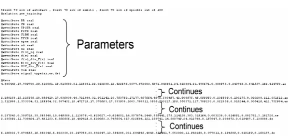
Figure 8. Weka Training Data Set. ...38
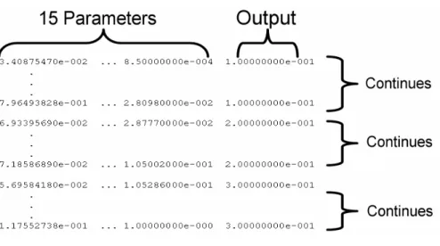
Figure 10. ANFIS Training Data Set. ...39
Figure 11. ANFIS Testing Data Set...39
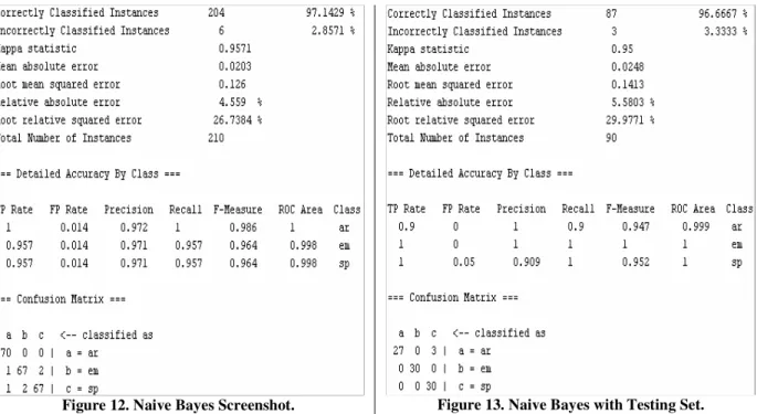
Figure 12. Naive Bayes Screenshot. ...40
Figure 13. Naive Bayes with Testing Set...40
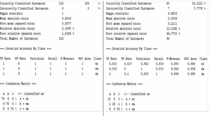
Figure 14. NBTree Screenshot. ...41
Figure 15. NBTree with Testing Set...41
Figure 16. LMT Screenshot. ...41
Figure 17. LMT with Testing Set. ...41
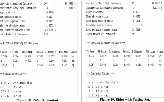
Figure 18. Ridor Screenshot...42
Figure 19. Ridor with Testing Set...42
Figure 20. Nnge Screenshot. ...42
Figure 21. Nnge with Testing Set. ...42
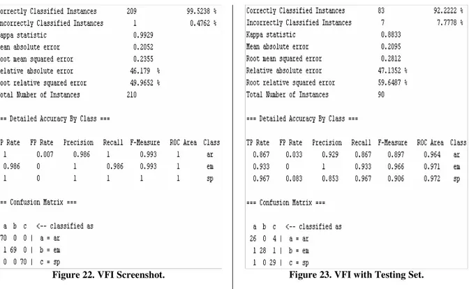
Figure 22. VFI Screenshot. ...43
Figure 23. VFI with Testing Set. ...43
Figure 24. Bagging Screenshot...43
Figure 25. Bagging with Testing Set. ...43
Figure 26. Dagging Screenshot. ...44
Figure 27. Dagging with Testing Set. ...44
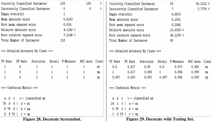
Figure 28. Decorate Screenshot...44
Figure 29. Decorate with Testing Set. ...44
Figure 30. Ada Boost M1 Screenshot. ...45
Figure 31. Ada Boost M1 with Testing Set...45
Figure 32. SMO Screenshot. ...45
Figure 33. SMO with Testing Set. ...45
Figure 34. Classification Via Regression Screenshot...46
Figure 35. Classification Via Regression with Testing Set...46
Figure 36. LWL Screenshot. ...46
Figure 37. LWL with Testing Set. ...46
Figure 38. Simple Logistic Screenshot. ...47
Figure 39. Simple Logistic with Testing Set...47
Figure 40. Multilayer Perceptron Screenshot...47
Figure 41. Multilayer Perceptron with Testing Set. ...47
Figure 42. RBF Network Screenshot...48
Figure 43. RBF Network with Testing Set...48
Figure 44. ANFIS Classification of Training Data...49
Figure 45. ANFIS Classification of Testing Data. ...49
Figure 46. Fuzzy Inference Diagram. ...50
Figure 47. Fuzzy Inference Diagram (continued). ...50
Figure 48. FIS Structure of the System...51
Figure 49. ROC Curve for Naive Bayes, ClassificationVia Regression, LWL, RBF Network, Multilayer Perceptron, and ANFIS. ...53
Figure 50. RMSE, Precision and Correctness Chart, sorted by ascending order of RMSE...56
Figure 51. RMSE, Precision and Correctness Chart, sorted by descending order of Precision...57
Figure 52. RMSE, Precision and Correctness Chart, sorted by descending order of Correctness. ...57
Figure 53. Sensitivity and Specificity Measures, sorted by descending order of Training Sensitivity...58
Figure 54. Sensitivity and Specificity Measures, sorted by descending order of
Training Specificity. ...58
Figure 55. Sensitivity and Specificity Measures, sorted by descending order of Testing Sensitivity. ...59
Figure 56. Sensitivity and Specificity Measures, sorted by descending order of Testing Specificity. ...59
LIST OF ALGORITHMS Algorithm 1. The Process of naive Bayes Method. ...10
Algorithm 2. The Process of Logit Boost Method. ...11
Algorithm 3. Ridor Algorithm...13
Algorithm 4. The Training Process of VFI Method. ...16
Algorithm 5. The Classification Phase of VFI Method. ...17
Algorithm 6. Bagging Algorithm. ...18
Algorithm 7. Decorate Algorithm...21
Algorithm 8. The Process of Ada Boost M1 Method. ...22
Algorithm 9. SMO Algorithm. ...23
Algorithm 10. Locally Weighted Regression Algorithm...26
Algorithm 11. The Process of RBF Network. ...32
Algorithm 12. ANFIS Algorithm. ...34
Algorithm 13. Cross Model Validation...36
LIST OF TABLES Table 1. Twelve Parameters with Threshold Values. ...6
Table 2. Average test Results of the Used Methods sorted as ascending order of RMSE...54
Table 3. Evaluation of Testing Specificity...55
LIST OF ABBREVIATIONS AR : Artifact Signal.
EM & ES : Embolic Signal.
SP & DS : Doppler Speckle Signal. DWT : Discrete Wavelet Transform.
DM : Data Mining.
VM : Veri Madenciliği.
NBTree : Naïve Bayes Tree. LMT : Logistic Model Trees. Ridor : Ripple Down Rules.
Nnge : Nearest Neighbor with Generalization. VFI : Voting Feature Interval.
Bagging : Bootstrap Aggregating. Dagging : Disjoint Aggregating.
Decorate : Diverse Ensemble Creation by Oppositional Relabeling of Artificial Training Examples.
SMO : Sequential Minimal Optimization. LWL : Locally Weighted Learning.
RBF Network : Radial Basis Function Neural Network. ANFIS : Adaptive Neuro Fuzzy Inference System.
1. INTRODUCTION
Asymptomatic circulating cerebral emboli, which are particles bigger than blood cells, can be detected by transcranial Doppler ultrasound. In certain conditions asymptomatic embolic signals (ES) appear to be markers of increased stroke risk . ES, reflected by an embolus, has some distinctive characteristics. They have usually larger amplitude than the signals from normal blood flow (Doppler speckle) and show a transient characteristic. They are finite oscillating signals and resemble wavelets. Unlike many artifacts such as caused by probe movement or speech, ES are unidirectional and usually contained within the flow spectrum. A number of methods to detect cerebral emboli have been studied in the literature. In Nebuya, et all, 2005, a phantom was constructed to simulate the electrical properties of the neck. A range of possible electrode configurations was then examined in order to improve the sensitivity of the impedance measurement method for the in vivo detection of air emboli. In Demchuk, et all, 2006, angiographically validated criteria for circle-of-Willis occlusion and thrombolysis in brain ischemia classification of residual flow have set the stage for the further development of Transcranial Doppler technique. In Chung, et all, 2005, the purpose of study was to improve reliability in the identification of Doppler embolic signals by determining the decibel threshold for reproducible detection of simulated "emboli" as a function of signal duration, frequency and cardiac-cycle position. In Okamura, et all, 2005, it has investigated that embolic particles could be detected as high-intensity transient signals with a Doppler guide wire during percutaneous coronary intervention in patients with acute myocardial infarction. In Girault, et all, 2006, in order to detect embolus, simple "off-line" synchronous detector has considered. In Kouame, et all, 2006, for
detection of microemboli with an expert knowledge, an autoregressive modeling associated with an abrupt change detection technique was used. In Palanchon, et all, 2005, instead of using Doppler techniques for emboli detection, a new technique has presented. This new technique consists of a multi-frequency transducer with two independent transmitting elements and a separate receiving part with a wide frequency band. In Mackinnon, et all, 2005, to determine patterns of embolization in two conditions and optimal recording protocols, ambulatory Transcranial Doppler system has applied to patients who have symptomatic and asymptomatic carotid stenosis. In Cowe, et all, 2005, Artifacts generated by healthy volunteers and embolic signals recorded from a flow phantom were used to characterize the appearance of two types of event. In Kilicarslan, et all, 2006, the relationship between microembolic signals, microbubble detection, and neurological outcome has discussed. In Rodriguez, et all, 2006, the effect of choosing different thresholds on the sensitivity and specificity of detecting high-intensity transient signals during cardiopulmonary bypass has investigated. In Dittrich, et all, 2006, the aim was installing primary and secondary quality control measures in clopidogrel and aspirin for reduction of emboli in symptomatic carotid stenosis. This is because microembolic signals evaluation relies on subjective judgment by human experts. In Chen, et all, 2006, main goal was to use multi-frequency transcranial Doppler to initially characterize emboli which is detected during carotid stenting with distal protection. In Rosenkranz, et all, 2006, the association of the number of solid cerebral microemboli during unprotected Carotid artery stent placement with the frequency of silent cerebral lesions which have detected by diffusion-weighted MR imaging has prospectively evaluated. In this study, data mining techniques have been used in order to increase sensitivity and specificity of an embolic signal detection
system previously described by Aydin, et all, 2004. Data mining techniques have been used in order to increase sensitivity and specificity of an embolic signal detection system. Similarly to the fuzzy approach, ANFIS has been used. Using sixteen methods in Weka and ANFIS, some results have been obtained. For the comparison purpose, testing specificity has been considered as the classification result of signals. Finally it has seen that these results were close or more accurate than the previous results in Aydin, et all, 2004.
1.1. Aim
In (Aydin, et all, 2004), main motivation was to detect asymptomatic emboli in arteries which may be an indication of stroke risk. For detecting asymptomatic emboli by using transcranial Doppler ultrasound signals, ES caused by emboli, DS caused by blood flow, and AR caused by other elements have been classified by fuzzy logic principle. The recorded signals from the patients consist of ES DS and AR. To distinguish ES from the others, a system consisting of DWT was developed (Aydin, et all, 2004). In this study, instead of using the fuzzy logic method, data mining techniques which is expected to enhance sensitivity and specificity of the previous system have been used.
2. BACKGROUND
A number of methods for detecting cerebral emboli using Doppler ultrasound have been studied in the literature. These include improving the sensitivity of the impedance measurement method for the in vivo detection of air emboli (Nebuya, et all, 2005), setting “Angiographically validated criteria for circle-of-Willis occlusion and thrombolysis in brain ischemia classification of residual flow” as stage for improvement of development of Transcranial Doppler technique (Demchuk, et all, 2006), improving reliability in the identification of Doppler embolic signals by determining the decibel threshold for reproducible detection of simulated "emboli" as a function of signal duration, frequency and cardiac-cycle position (Chung, et all, 2005), investigating whether embolic particles could be detected as high-intensity transient signals with a Doppler guide wire during percutaneous coronary intervention in patients with acute myocardial infarction (Okamura, et all, 2005), and considering a simple "off-line" synchronous detector to detect embolus (Girault, et all, 2006). The previous work (Aydin, et all, 2004) was about detection of asymptomatic emboli in arteries that could have been an evidence of stroke risk. To be able to detect emboli, fuzzy logic detection system was used. However, there are other kind of signals. Those are DS and AR and which are mixed with ES. In order to distinguish ES, these three signals must be analyzed. ES is a high intensity signal resulted from emboli particles. AR is produced by tissue movement, speaking, probe tapping, etc. DS is caused by blood flow. Usually, the bandwidth of ES is narrower than DS. Briefly, the process of the data preparation and fuzzy detection are given as follows:
1) The signals from 35 patients having symptomatic carotid stenosis were recorded by using a transcranial Doppler ultrasound system (Pioneer TC4040).
2) These recorded quadrature audio Doppler signals including ES were exported to a PC.
3) In order to evaluate feasibility of these signals, two independent data sets each including 100 ES, 100 AR and 100 DS were used.
4) After applying 8 order DWT to the exported data, 15 parameters which have ES, AR and DS each, were evaluated. In Table 1, 12 of these 15 parameters are shown.
5) Then, threshold values which are identified before were applied to each of the fifteen parameters.
6) At last; using output which was resulted from fuzzy logic, another fuzzy logic detection has been performed as well. Therefore, ES, AR and DS were classified. From the first data set, while ES has been detected as 98%, from the second data set, ES has been detected as 95%. In this study, the second result is considered and compared with results of used DM methods. Although the DWT coefficients of scales 5-6-7-8 were dominated by AR, the DWT coefficients of scales 1-2-3-4 were dominated by ES and DS.
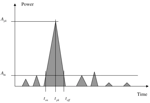
P2TR means the scale with maximum peak to threshold ratio. TP2TR indicates the total power to the threshold ratio. RR is the ES rise rate; FR is the ES fall rate. F2RM indicates peak forward to reverse power ratio. TF2R means total forward to reverse power ratio. Ts2 is time spreading term and
2 s
B is the frequency spreading term. VIE and VIF are algorithm variances as instantaneous envelope of signals and
instantaneous frequency of signals, respectively. ts is the average time of the signal
and fs is the average frequency of the signal, respectively. s(t) is the probability
distribution.S( f)is the Fourier transform of s(t).
Table 1. Twelve Parameters with Threshold Values.
th1 th2 th3 th4 (dB) 2TR P 6 12 14 20 (dB) 2TR TP 17 23 26 38 (dB) 2RM F 10 20 22 26 TF2R(dB) 4 8 10 20 (ms) RR 0.6 1.4 2 5 (ms) FR 0.6 1.4 2 6 (ms) s t 10 20 60 120 ) unit ( / s s F f 0.01 0.035 0.08 0.1 ) (ms2 2 s T 6 18 40 100 (unit) / 2 s s F B 0.03 0.06 0.1 0.4 (unit) VIE 12 60 100 140 (unit) /Fs VIF 0.008 0.016 0.021 0.04
The thresholds are obtained by statistical evaluation of the ES, DS and AR (Aydin, et all, 2004). These thresholds are used in fuzzy logic.
Figure 1. A Representative Constructed Wavelet Scale Containing an ES and Quantities to Calculate Parameters.
In (1) and (2), the mathematical representations of the parameters are given. Af(k) and Ar(k) are instantaneous power (IP) of forward and reverse signals, respectively.
) ( log 10 2 dB A A TR P th pk
= where Apkand Athare IP forward and reverse signals, respectively. ) ( ) ( log 10 log 10 2 db A k A A A TR TP th t t k f th tot off on
∑
= = = ) / ( 2 log 10 ms dB t t TR P t t A A RR on pk on pk th pk − = − = ) / ( 2 log 10 ms dB t t TR P t t A A FR pk off pk off th pk − = − = ) ( ) ( ) ( log 10 2 dB k A k A R TF off ın off on t t k r t t k f∑
∑
= = = (1) In (2), it is continued. pk t toff on t Time Power pk A th Adt t s t E t s s 2 ) ( 1
∫
∞ ∞ −= where ts is the average time of the signal. s(t) is the probability distribution. df f S f E f s s 2 ) ( 1
∫
∞ ∞ −= where S(f) is the fourier transform of s(t). S(f) is the average frequency of the signal.
dt t s t t E T s s s 2 2 2 ) ( ) ( 1
∫
∞ ∞ − − =( )
f df S f f E B s s s 2 2 2 ) ( 1∫
∞ ∞ − − = where =∫
<∞ ∞ ∞ − dt t s Es 2 ) ( (2)Data mining is a multidisciplinary field of research and development of algorithms and software environments to support this activity in the context of real-life problems where often huge amounts of data are available for mining. Data mining is sometimes considered as just a step in an overall process called Knowledge
Discovery in Databases, KDD. Data mining includes a large set of technologies,
including data warehousing, database management, data analysis algorithms and visualization (Apte, et all, 1997), (Mullins, et all, 2006). In this study, seventeen data mining methods have been used. By using DM methods in detection of emboli, it is expected to increase the sensitivity and specificity of the system in previous work. The detailed descriptions of these seventeen methods have been given as below.
2.1. Naive Bayes
Bayesian networks are a popular medium for graphically representing and manipulating attribute interdependencies and represent a joint probability distribution over a set of discrete, stochastic variables. Bayesian classification has been widely used in many machine learning applications, also in medical diagnosis. The Bayesian approach searches in a model space for the “best” class descriptions. A best classification optimally trades off predictive accuracy against the complexity of the
classes, and so does not overfit the data. Such classes are also fuzzy, instead of each case being assigned to a class, a case has a probability of being a member of each of the different classes.
Bayesian networks have several advantages for data analysis. Firstly, since the model encodes dependencies among all variables, it readily handles situations where some data entries are missing. Secondly, a Bayesian network can be used to learn causal relationships and hence can be used to gain understanding about a problem domain and to predict the consequences. Thirdly, because the model includes both causal and probabilistic semantics, it is an ideal representation for combining prior knowledge, which often comes in causal form and data. Fourthly, bayesian statistical methods in conjunction with bayesian networks offer an efficient and widely recognized approach for avoiding the over-fitting of data. Finally, it is found that diagnostic performance with Bayesian networks is often surprisingly insensitive to imprecision in the numerical probabilities. Bayesian networks are directed acyclic graphs that allow for efficient and effective representation of joint probability distributions over a set of random variables.
The Naive Bayesian Classifier is one of the most computationally efficient algorithm for machine learning and data mining. The naive Bayesian classifier is a bayesian network, used for classification. It is a probabilistic approach to classification. Compared with neural networks, decision trees, clustering and regression, the naive bayesian classifier is a simple and, effective classifier. For example, in medical area, mineral potential mapping is used as naive bayesian classifier. Belonging to the bayesian network classifier, bayesian classifier predicts a class C for a pattern x. The expression of the Bayesian Classification is shown in equation (3) (Ouali,et all, 2005).
(
)
(
)
( )
(
X x)
p C P C x X p x X C P = • = = = (3)2.2. Naive Bayes Tree (NBTree)
Naive Bayes Tree (NBTree) algorithm is a hybrid approach when many attributes are likely to be relevant for a classification task. NBTree is similar to the classical recursive partitioning schemes, except that the leaf nodes created are Naive Bayes categorizers instead of nodes predicting a single class. A threshold for continious attributes is chosen using the standard entorpy minimizatioin technique, for decision trees. NBTree uses decision tree techniques to partititon the whole instance space (root node) into many subspaces (leaf nodes) then trains Naïve Bayes classifier for each leaf node. NBTree produces highly accurate classifiers. In Algorithm 1, the process of Naive Bayes Tree is shown (Kohavi, et all, 1996), (Fonseca, et all, 2003), (Xie, et all,2004).
Algorithm 1. The Process of naive Bayes Method. 1) For each attribute
x
i, evaluate u(xi) of a split on attribute xi.2) Let j=argmax(ui) (The attribute with highest value).
3) If uj is significantly not better than the utility of the current node, create a Naive Bayes Classifier for the current node and return.
4) Partition T according to the test on xj. If xj is continuous, a threshold split is used ; if xj is discrete, a multi-way split is made for all possible values.
5) For each child, call the algorithm recursively on the portion of T that leads to the child.
2.3. Logistic Model Trees (LMT)
Model trees predict a numeric value which is defined over a stationary set of numeric or nominal attributes. Unlike regression trees, model trees produces piecewise linear approximation to the destination function. At the end, the final model tree includes a
decision tree with linear regression models at leaves also the prediction of instance is gathered with using the prediction of the linear model that is associated with the leaf. Unsimilarly with model trees, Logistic Model Trees or LMT employs an efficient and flexible approach for building logistic models using the well-known CART algorithm for pruning. The process of LMT starts by building a logistic model at the root using LogitBoost algorithm. The pseudocode for LogitBoost algorithm is shown in Algorithm 2.
Algorithm 2. The Process of Logit Boost Method. 1. Start with weights
wij =1/N, i =1,K,N ,j=1,K,J ,Fj(x)=0andpj(x)=1/J 2. Repeat for ∑ = = + ← − − ← − = − − = = =
∑
= J k k x F e m j F e x x Fit c x f x F x F x f J x f J J x b ii x p x p x p x p x p y a M m mj j J k mk j mj i j i j i j i j i j ij 1 ( ) ) ( ) ( j p Update Set ij w hts with weig i x to ij z of regression squares least weighted a by ) ( mj f function the class jth in weights and responses working Compare ) ) ( ) ( ) ( )), ( 1 ) ( ( 1 ) ( f ) . )) ( 1 )( ( w , )) ( 1 )( ( ) ( z i. : J , 1, j for Repeat ) : , , 1 1 mj ij ij K K3. Output the classifier argmaxjFj(x).
The iterations are determined by using five fold cross validation. The data is split into training and test as five times. Logit Boost algorithm is run to a maximum number of iterations. Next, the error rates on test set are gathered then summed up over different folds. After that, the number of iterations with the lowest sum of errors
is used to train the LogitBoost algorithm. This process is called the logistic regression model, at the root of the tree. The formulation of linear logistic regression is
∑
∑
= = = = = = J 1 k 1 ) ( ) ( , 0 ) ( , ) | Pr( F x e e x X j G J k k x F x F k j (4)where Pr(G=j|X=x) is the pasterior class probability for J classes with functions x and Fj(x)=βjT.x. Therefore, considering binary splits on numerical attributes and multiway splits, on nominal attributes, by using C4.5 algorithm, a split of the data at the root is constructed. The LogitBoost algorithm is run on child node by starting with the committee Fj(x), weights wij and probability estimates pij of the last
iteration. The splitting continues as long as 15 instances are at a node. Finaly, the tree is pruned using CART pruning algorithm (Landwehr, et all, 2003).
2.4. Ripple Down Rules (Ridor)
RIpple-DOwn Rule or Ridor is a knowledge acquisition technique. The major
feature of ripple down rules is, first, they can be added to a knowledge base faster than relational rules since the rules are added without modification. Secondly, since ridor is only used in context, they have less impact in damaging the knowledge base. With ridor, redundancy is the major problem because since knowledge is entered in context, the similar rule may end up being repeated in multiple contexts. Ripple Down Rules create exceptions to existing rules so changes are bounded in the context of the rule and will not affect other rules. Ripple Down Rules look like decision lists which are in the form if-then-else as new RDR rules are added by creating except or else branches to the existing rules. If a rule fires but produces an incorrect conclusion
then for the new rule, an except branch is created. If no rule fires then an else branch is created for the new rule. The simplest Ridor pseudocode is shown in Algorithm 3.
Algorithm 3. Ridor Algorithm. 1) If a^b then c
2) except if d then e 3) else if f^g then h
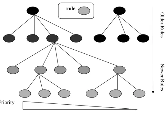
The rule is implemented as, if a and b are true then we conclude c unless d is false. If d is false, we conclude e. If a and b are not true we continue with other rules that if f and g true then we conclude h. In order to create an exception to a rule, the algorithm should recover the word which caused the rule fired. In Figure 2, we can see the process of Ridor. The two black ellipses at the root are LAST_FIRED(0) rules. The process is considered one by one, left to right. To implement the fire, the prediction for either of these rules is “no other rule has fired”. The rule on the left is considered first. If it doesn’t fire, the next oldest LAST_FIRED(0) is considered. If a LAST_FIRED(0) rule does fire then in the next level, only the rules connected to it are applicants to fire. The newest against the oldest is added. Once one of these child rule is added then the only rules connected to it are net ones to fire (Compton, et all, 1990).
Figure 2. Representation of Ripple Down Rules.
In Industry, the variation of Ridor rules such as Multiple Classification of Ripple
Down Rules (MCRDR) is developed. MCRDR incrementally and rapidly acquires
and validates the knowledge which is on case by case criteria. Cases are used to validate the acquired knowledge (Richards, et all, 2002).
2.5. Nearest Neighbor with Generalization (Nnge)
Nearest Neighbor with Generalization (Nnge) is the Nearest Neighbor like algorithm, using non-nested generalized attributes. If the data is randomly spreaded, the algorithm employs the ratio “R” to the mean expected distance. This ratio R can be used for the three moments of the expected distance: the mean expected distance, the standard deviation of expected distance and the skewness of the frequency distribution of these distances. In k dimensional space, these three moments can be
rule O lde r R ul es N ew er R ul es Older Rules Newer Rules Priority
derived for a random dispersion of individuals. As the spherical volume of the sphere is given by ) 1 ) 2 / (( 2 / + Γ = k r V k k sp π (5)
the probability of sphere that doesn’t contain no other individual is
) 1 ) 2 / (( 3 / + Γ −
∏
k r e k k ρ (6)where ρ is the density of the population. This equation is also called the amount of distances to nearest neighbor, greater than r. Instead of nearest neighbor algorithm, Nnge obtains outputs from regular exemplars (Clark, et all, 1979). In (Pignotti, et all, 2004), Service Predictor and Alert System predicts the next service and checks whether time and user’s location are appropriate or not. For the system, sequence rules do not provide time and location information to the user. By using NNGE, proximity rules which have time and location information to the user is generated.
2.6. Voting Feature Interval (VFI)
Voting Feature Interval (VFI) is the method for implementing the Voting Feature Interval classifier. VFI is faster than NaiveBayes algorithm. For VFI, each training example is represented as a vector of feature values with a label representing the class of the example. From the training examples, VFI constructs feature intervals for each feature. A feature interval represents a set of values of a given feature where the same subset of class values is observed. Two neighboring intervals contain different sets of intervals. The training process of VFI is given in Algorithm 4. In the training phase of VFI, the feature intervals for each feature dimension are constructed. The procedure find_end_points(TrainingSet,f,c) finds the lowest and the highest values
for linear feature f from the examples of class c and each observed value for nominal feature f from the examples in TrainingSet. For each linear feature, 2k values are found. k is the number of classes. Next, the list of 2k end-points is sorted and each consecutive pair of points selects a fair interval. Each interval is represented by a vector of lower,count1,K,countk where lower is the lower bound of that interval and counti is the number of training instances of class i falling into that interval. The count values are computed by count_instances(i,c). i
Algorithm 4. The Training Process of VFI Method. train(TrainingSet):
begin
for each feature f for each class c
EndPoints[f]=EndPoints[f]∪find_end_points(TrainingSet,f,c); sort(EndPoints[f]);
for each class c
interval_class_count[f,i,c]=count_instances(f,i,c); end
The classification phase of the VFI algorithm is given in Algorithm 5. The process starts by initializing the votes for each class by zero. ef is the f value of the test
example e. For each feature f, the interval on feature dimension f which ef falls into, is searched. If ef is missing, the corresponding feature gives a vote zero for each class. Thus, the features containing missing values are simply ignored. If ef is known, the interval i which ef falls into, is found. For each class c, feature f gives a
vote equal to
[
]
[
]
[ ]
c count _ class c , i , f lass_count interval_c c , f vote _ feature = (7)where interval_class_count[f,i,c] is the number of examples of class c which fall into interval i of feature dimension f. Each feature f collects its votes in an individual vote vector votef,1,K,votef,k , where votef,c is the individual vote of feature f for class c. k is the number of classes. Then, the individual vote vectors are summed up to get a total vote vector vote1,K,votek . At last, the class with the highest total vote is predicted to be the class of the test instance (Demiroz, et all, 1997). In industry, VFI can be used for signal analysis such as noise analysis of network problems (Kalapanidas, et all, 2003).
Algorithm 5. The Classification Phase of VFI Method. classify(e):
begin
for each class c vote[c]=0 for each feature f
for each class c
feature_vote[f,c]=0 if efvalue is known i=find_interval(f,ef)
[ ]
[
]
[ ]
c count _ class c , i , f count _ class _ interval c , f vote _ eature f = normalize_feature_votes(f); for each class cvote[c]=vote[c]+feature_vote[f,c]; return class c with highest vote[c];
end
2.7. Bootstrap Aggregating (Bagging)
Bootstrap Aggregating (Bagging) is the method of stacked generalization in combining models derived from different subsets of a training dataset by a single learning algorithm. Given a training dataset T of size N, standard batch bagging
creates M base models. Each model is trained by calling the batch learning algorithm
b
L on a bootstrap sample of size N which is created by drawing random samples with replacement from original data set. The pseudocode of bagging is given in Algorithm 6 (Oza, et all, 2005).
Algorithm 6. Bagging Algorithm. Bagging(T,Lb,M) For each m ∈ {1,2,...,M}, m T = Sample_With_Replacement(T,|T|) m h =Lb(Tm) Return{h1,h2,...,hm}
In order to combine predictions from different models derived from a single learning algorithm, majority vote is used. Bootstrap samples are randomly sampling L with replacement into K subsets of size N. Bootstrap samples are used in order to deliver training subsets. Let us we have a learning set L=
{
(
yn,xn)
,n=1,K,N}
where y’sare either class labels or numeric response. And let us call ϕ
(
x,L)
a predictor. If the input is x, we predict y by ϕ(
x,L)
. Now, let us we are given a sequence of learning sets{ }
Lk , each including of N independent observations from the same underlying distribution as L. Our aim is to use the Lk to get a better predictor than the single learning set predictor ϕ(
x,L)
. If y is numerical, then we can replace ϕ(
x,L)
by the average of ϕ(
x,Lk)
over k. If ϕ( Lx, ) predicts a class j∈{
1 K, ,J}
, then we can gather ϕ(
x,Lk)
by voting. Let Nj =#{
k;ϕ(
x,Lk)
= j}
and takeϕA(x)=argmaxj Nj. Let us take repeated bootstrap samples( )
{ }
B L from L then form{
(
( )B)
}
L x, ϕ . If y is numerical, we take ϕ as B ( )(
, ( )B)
. B B x av ϕ x L ϕ = . If y is aclass label, let
{
( )B}
L x,
(
ϕ vote to form ϕB
( )
x . This procedure is called “Bootstrap Aggregating” or Bagging (Breiman,et all., 1996).2.8. Disjoint Aggregating (Dagging)
Dagging stands for Disjoint Aggregating. In Dagging, similar to bagging, it uses majority vote to combine multiple models, obtained from a single learning algorithm. Unlike bagging, dagging uses disjoint samples, rather than bootstrapping. The training set is partitioned into k subsets. A base classifier generates a hypothesis for each subset. The final prediction is done by plurality vote as same in bagging. Another difference is, dagging doesn’t use extra resources since the same amount of examples are used as the training set (Tate, et all, 2005). Let us we have I output classes and let pki(x) denote the probability that the kth model assigns to the ith
class that is given the test instance x. The vector
( )
( )
( )
(
n n n)
kn pk x pki x pkI x
P = 1 ,K, ,K, (8)
gives the k model’s class probabilities for the th n instance. At the end of the th
testing, data evaluated from the output of the K models is
(
)
{
y p p p n N}
L~= n, 1n,K, kn,K, Kn , =1,K, ′ (9)
This is called level-1 data. Using a learning algorithm that is called level-1 generalizer, we obtain a model M~ called level-1 model that predicts the class from
this level-1 data. In order to classify a new instance, the level-0 models Mk are used to produce a vector
(
p11,K,p1I,K,pk1,K,pkI,K,pK1,K,pKI)
that is input to theM~ and the output M~ is the final classification result of it. Depending on the sampling strategy used to produce the data derived from level-0 models, we call thisimplementation Stacked Generalization Bag Stacking or Dag Stacking (Ting, et all, 1997).
2.9. Diverse Ensemble Creation by Oppositional Relabeling
of Artificial Training Examples (Decorate)
Decorate, stands for Diverse Ensemble Creation by Oppositional Relabeling of Artificial Training Examples. The combination of the output of several classifiers is useful if they disagree on some inputs. This disagreement is referred as diversity of the ensemble. For regression problems, generally, mean squared error is used to measure accuracy while the variance is used to measure diversity. The generalization error E of the ensemble can be expressed as E =E −D where E and D are mean error and diversity of the ensemble, respectively. Let us call Ci(x) as the prediction of the ithclassifier for the label of x. And let us call *( )
x
C as the prediction of the
entire ensemble. The diversity of the i-th classifier is evaluated on example x as
(10)
To compute the diversity of an ensemble of size n on a training set of size m, the above term is averaged:
∑∑
= = = n i m j j i x d nm 1 1 ) ( 1 (11) In Decorate algorithm, an ensemble is generated iteratively. First, learning a classifier then adding it to the current ensemble is performed. In Algorithm 7, Decorate algorithm is shown. The classifiers in each successive iteration are trained on the original training data. In each iteration, artificial training examples are generated from the data distribution. Rsize is the number of examples to be generated.= ) (x di Otherwise : 1 ) ( C ) ( C If : 0 * i x = x
Decorate has much more accurate than Bagging and Boosting algorithms (Merville, et all, 2004).
Algorithm 7. Decorate Algorithm.
(
)
(
)
{ }
1 trials trials 19) } C { * C * C 18) otherwise, 17) 16) 1 i i 15) e If 14) 5 step in as * C of e error training Compute 13) data artificial the remove , R T T 12) } C { * C * C 11) T) BaseLearn( C 10) R T T 9) * C of s prediction to al proportion inversely labels class of y probabilit with R in examples Label 8) data training of on distributi on based R examples training T size R Generate 7) max I trials and size C i While 6) m j y ) j (x * C T, xj 1 error ensemble Compute 5) i C * C ensemble Initialize 4) T) BaseLearn( i C 3) 1 trials 2) 1 i 1) . generation for examples artificial of number determines t Factor tha : size R . ensemble an build to iterations of number Maximum : max I size. ensemble Desired : size C Y j y labels with m y , m x , , 1 y , 1 x examples training m of Set : T algorithm. Learning Base : BaseLearn : Input + = ′ − = ′ = + = ≤ ′ ′ − = ′ ∪ = = ′ ∪ = × < < ∑ ∈ ≠ ∈= = = = = ∈ e e e K2.10. Ada Boost M1
In order to improve the classification accuracy, AdaBoost algorithm has been theoretically proved to be an effective method. It focuses on minimization of training errors. However, when data is noisy, AdaBoost might have problem with overfitting (Jin, et all, 2003). AdaBoost.M1, which is the variation of AdaBoost algorithm can be used to improve the performance of a learning algorithm. Or it can be used to reduce the error of a classifier. The boosting algorithm AdaBoost.M1 takes a training set of m examples
(
)
(
)
{
x
y
x
my
m}
S
=
1,
1,
K
,
,
(12)as input. xi is an instance drawn from some space x and it is a vector of attribute values. yi∈ is the class label, associated with Y xi. The boosting algorithm calls a
learning algorithm, called WeakLearn, in many times. The aim of the weak learn algorithm is to find a value h which minimizes the training error. The disadvantage t of AdaBoostM1 is, when the training error is greater than 0.5, algorithm cannot handle with weak values of ht. In Algorithm 8, the process of AdaBoostM1 is shown (Freund,et all, 1996).
Algorithm 8. The Process of Ada Boost M1 Method. 1) Call weakLearn, providing distribution Dt, 2) Get back hypothesis ht X→Y, 3) Calculate the error of ht,
2.11. Sequential Minimal Optimization (SMO)
The Support Vector Machine (SVM) algorithm is a classification technique. Given training vectors xi∈Rn,i=1,K,l in two classes and a vector y∈Rl like ∈
{
1 −, 1}
i
y ,
SVM gives the following problem
0 , , , 1 , 0 2 1 min i = = ≤ ≤ − α α α α α T T T y l i C e Q K (13)
where e is the vector of all ones, C is the upper bound of all variables and Q is an l by l positive semi definite matrix (Lin,et all, 2000). Before we understand the Sequential Minimal Optimization (SMO) algorithm, let us examine the Support Vector Machine Quadratic Programming or SVM QP. SVM QP is known as chunking. The chunking algorithm uses the fact that if you remove the rows and the columns of the matrix corresponding to zero multipliers, the value of the quadratic form is the same. Thus, the large QP problem can be broken down into series of small QP problems whose main goal is to detect all of the non zero Lagrange multipliers and discard all of the zero Lagrange multipliers. Sequential Minimal Optimization is the simple algorithm that can rapidly solve the SVM QP problem without any extra matrix storage and without using numerical QP optimization steps at all. In Algorithm 9, the SMO algorithm is shown.
Algorithm 9. SMO Algorithm. 1) Divide QP problem into partitions,
2) Choose and solve smallest optimization on at every step,
3) Choose two Lagrange multipliers, find optimal values for these multipliers, 4) Update SVM.
SMO divides the overall QP problem into QP sub problems. Unlike other methods, SMO chooses to solve the smallest possible optimization problem at every step. At every step, SMO chooses two Lagrange multipliers to optimize and finds optimal values for these multipliers then updates the SVM to reflect the new optimal values. The advantage of SMO comes from easily solving two Lagrange problems, analytically. In addition, SMO does not require no extra matrix storage at all. SMO can be changed to solve fixed threshold SVM’s. SMO updates individual Lagrange multipliers to be the minimum value of function Ψ along the corresponding dimension. The update rule is
(
1 1)
1 1 1 1 x x K E y new r r + =α α (14)where α is the Lagrange multiplier, Ei is the training error in ithexample K is the kernel x is input and y is the target. This update equation forces the output of SVM to be y (Platt,et all,1998). In some areas, the implementation of SMO algorithm such 1
as SMOBR which is written in C++ is used to work with data sets such as with data sets on hyperplanes (Kornienko, et all, 2005). In test results, SMOBR has shown better performance than other SVM methods.
2.12. Classification via Regression
This method uses regression methods C5.0, M5.0 and LR to perform classification. At the leaves, model trees execute the process of predicting continuous numeric values by using function approximation. For better understanding, let us consider we have a model at a leaf involved two attributes x and y with linear coefficients a and b and the model at the parent node involved two attributes y and z are
by ax
p= + (15)
dz cy
q= + (16)
In Classification via Regression, these two models are come together with formula z k n kd y k n kc nb x k n na p + + + + + + = ′ (17)
where p′ is the prediction passed up to the next higher node. p is the prediction passed to this node. q is the value predicted by the model at this node. n is the number of training instances which reach the node below and k is the constant. It continues until root gives a single smoothed linear model that will be used for the prediction (Frank, et all, 1998). Classification via Regression is used in biological areas for example in Langdon, et all, 2003, it is used in genetic programming to investigate the biochemical interactions with human P450 2D6 enzyme.
2.13. Locally Weighted Learning (LWL)
LWL stands for Locally Weighted Learning. In LWL, linear regression model is fit to the data that is based on a weighting function and centered on the instance where a prediction is about to be generated. The resulting estimation is linear. To illustrate how locally weighted learning works, let us consider distance weighted averaging. Equation (18) is locally weighted regression because the local model is constant. A prediction yˆ can be based on an average of n training values
{
y1,y2,K,yn}
isn y
yˆ=
∑
i (18)this estimate minimizes a criterion:
(
)
2 ˆ∑
− = i i y y C (19)In the case where the training values
{
y1,y2,K,yn}
are taken under differentfit to nearby data. LWR can be derived by either weighting the training criterion for the local model or by directly weighting the data (Atkenson, et all,1997). Training of LWR is fast. It just requires adding new training data to the memory. When a prediction is needed for a query point x , the following weighted regression analysis q
is performed:
Algorithm 10. Locally Weighted Regression Algorithm. Given:
A query point qX and p training points
{
xi,yi}
in memory. Compute Prediction:a)Compute diagonal weight matrix W where
(
) (
)
− − − = xi xq TDxi xq 2 1 exp ii wb)Build matrix X and vector y such that
(
)
[
(
)
T]
T q x i x i x where T p x , , 2 x , 1 x X= ~ ~ K ~ ~ = −(
)
T p y , , 2 y , 1 y y= Kc)Compute locally linear model
(
XTWX)
1XTWyβ= −
d)The prediction for xq is thus 1 n β q y = + ˆ 1 + n β denotes th n 1)
( + element of the regression vector β (Schaal,et all,2002). Locally weighted learning is critically dependent on the distance function. The three distance functions are Global Distance Functions, Query-based Local Distance Functions and Point- based local distance functions. Global distance functions are used in input space. For Query based local distance functions, the distance function, d() parameters are set on each query by an optimization process which typically minimizes the cross validation error. In point based local distance functions, the training criterion uses a different d() for each point xi:
(
)
(
(
)
)
[
]
∑
− = i i i i i y K d x q x f q C( ) ( ,β )2 , (20)the di() can be selected either by a direct computation or by minimizing cross validation error. In locally weighted learning, it is possible to estimate the prediction error and gather confidence bounds in the predictions. LWL shows robust effects according to its most important parameter, the neighborhood size (Atkenson, et all, 1997).
2.14. Simple Logistic
Simple Logistic is the class for building a logistic regression model, using LogitBoost. The Logistic Regression Model Boosting is performed by applying a classification algorithm to reweighted type of training data and then giving a weighted majority vote of the sequence of classifiers. LogitBoost performs classification using a regression scheme as the base learner using additive logistic regression. The additive logistic regression has the form
∑
==
p j j jx
f
x
F
1)
(
)
(
(21)each component of fj is a function belonging to small subset of variables xj. The logistic regression model is used when the response variable of interest takes on two values (Friedman, et all, 2000). Let us define a response variable as y and denote event as y=1 when the subject has the characteristic of interest and y=0 when the subject does not. Also let us suppose the subject has a single predictor x that could be related to the response. The logistic regression defines the probability P(y=1) as,
(
)
(
x)
x y P 1 0 1 0 exp 1 ) exp( 1 β β β β + + + = = (22)(
)
) exp( ) 0 ( ) 1 ( ) 1 ( 1x y P y P y odds = β +β = = = = (23)
meaning that the odds is simply the linear function β +0 β1x. This model has two parameters (Anderson, et all, 2002).
2.15. Back Propagation
Many neural network algorithms aim to adjust the weights to get better results in the performance. The gradient is evaluated using the technique, back propagation. The back propagation updates network weights and biases in the direction of performance function that decreases more rapidly.
k k k
k
X
g
X
+1=
−
α
(24)In equation (24), X is a vector of current weights and biases, k g is the current k gradient and αk is the learning rate. The gradient is evaluated as
e
J
g
=
T (25)In equation (25), g is gradient, J is jacobian matrix which has the derivatives of network errors with respect to weights and biases, e is a vector of network errors. And the hessian matrix is shown as
J
J
H
=
T (26)Moreover, similar approach to evaluate weights and biases;
[
J
J
I
]
J
e
X
X
k+1=
k−
T+
µ
−1 T (27)When µ is zero, the gradient descent reduces with a small step size (Yan,et all, 2003).
2.16. Multilayer Perceptron
Multilayer Perceptron is a method which uses backpropagation to classify instances. Except for when the class is numeric, the nodes in this network are all sigmoid. In this case the output nodes become unthresholded linear units. The architecture of Multilayer Perceptron is given in Figure 3.
Perceptrons
A typical multilayer perceptron network consists of three or more layers of processing nodes; an input layer that receives external inputs, one or more hidden
layers, and an output layer.
Figure 3. Architecture of a Multilayer Perceptron Network.
Process of Multilayer Perceptron
In the input layer, no process is done. When data are presented at the input layer, the network nodes perform calculations in the successive layers until an output value is obtained at each of the output nodes. This output signal should be able to indicate the
...
...
...
Hidden Layer(s) Input Layer Output LayerOutput Classes yi Level
j
k
i
Input Pattern Feature Value xi Connection Weights
appropriate class for the input data. That is, one can expect to have a high output value on the correct class node and low output values on all the rest. On Figure 4, a node in multilayer perceptron can be modeled as an artificial neuron which computes the weighted sum of the inputs at the presence of the bias, and passes this sum through the activation function as equation (28)
Figure 4. One Node of Multilayer Perceptron; an Artificial Neuron.
∑
==
+
=
p i j j j i ji jw
x
f
v
v
1 j(
)
y
θ
(28)where
v
j is the linear combination of inputsx
1,
x
2,...,
x
p,
θ
j is the bias,w
ji is the connection weight between the inputx
i and the neuron j, and fj( )
vj is theactivation function of the
j
th neuron, and yj is the output. The sigmoid function isa common choice of the activation function (Yan, et all, 2003);
a
e
a
f
−+
=
1
1
)
(
(29)∑
f(.
) 1 x 2 x 3 x p x 1 j w 2 j w 3 j w jp w...
Bias (qj)=1 i y2.17. Radial Basis Function Neural Network (RBF NN)
Radial Basis Function Neural Network or RBF Neural Network is developed by using stochastic gradient descent method and a supervised clustering method. Unsupervised learning algorithms of RBF NN appear naturally suited. The structure of RBF Neural Networks is modular and can be easily implemented to hardware. RBF NN method is a normalized Gaussian Radial Basis Function Network. RBF Network uses the k-means clustering algorithm to provide the basis functions and learns either a logistic regression for discrete class problems or linear regression for numeric class problems. RBF Network standardizes all numeric attributes to zero mean and unit variance. The RBF network has three layers: an input layer, a single layer for nonlinear processing of neurons and output layer (Tan, et all, 2001). In Figure 5, RBF Network with three layers is shown. For every input, every gaussian unit in hidden layer evaluates its output as a function of its center and width (variance).
Figure 5. RBF Network with three Layers.
The input for RBF network is
0 G G1 G2
...
Gg−1...
...
X0 X1 X2 X(n) y0 y1 y(n) Input Layer Single Layer Output Layerj k b c x j j e b x G 2 2 2 2 1 ) ( − − = π (30)
where x are inputs, Gj(x) is the output of the j unit, th cj is the center of the unit j and bj2 is the variance of the
th
j unit. The overall output is calculated as weighted sum of outputs of hidden units
m , 1,2, i , ) c x ( φ w ) c (x, φ w (x) f y N 1 k N 1 k 2 k k ik k k ik i i = =
∑
=∑
− = K = = (31) where ×1 ∈ n Rx is input vector, φkis the function from +
R and . denotes the 2 euclidean norm, wik are the weights of output layer, N is the number of neurons in the hidden layer and ∈ n×1
k R
c are RBF centers in input space. The process of RBF Network is given in Algorithm 11. The process starts by initializing the weights. For each neuron in hidden layer, the euclidean distance between its associated center and input to the network is computed. At last, the output of the network is computed as a weighted sum of hidden layer outputs. In addition, the weights are updated (Isa, et all, 2005).
Algorithm 11. The Process of RBF Network. 1) Initialize weigths,
2) For each neuron in hidden layer evaluate its euclidean distance, 3) Evaluate weighted sum of hidden layers,
4) Update weights, 5) Go to step 5.
3. Adaptive Neuro Fuzzy Inference System (ANFIS)
ANFIS stands for Adaptive Neuro Fuzzy Inference System. It is a fuzzy modeling procedure to learn about a data set and its aim is in order to compute the membership function parameters that best allow the corresponding fuzzy inference system to follow the given input - output data. Using a given input - output data set, ANFIS constructs a fuzzy inference system, FIS. Its membership function parameters are tuned using a backpropagation algorithm. This algorithm is single or with combination of least squares type of method. This allows fuzzy systems to learn the data they are modeling. In ANFIS, first, you hypothesize a parameterized model structure, relating inputs to membership functions, and to rules. Next, for training, you collect input - output data, that is in usable format by ANFIS. At last, the data which is delivered by modifying membership parameters, is trained by ANFIS. ANFIS is not available for all of the fuzzy inference system options. ANFIS only supports sugeno - type systems, having the following properties: First, it has the first order or zeroth order sugeno type systems. Second, it has a single output, obtained by weighted average defuzzification. All output functions must be in the same type or linear & constant. Third, it has no rule sharing. Different rules cannot share the same output membership function. And finally, ANFIS has unity weight for each rule. If any of these four rules is not accomplished, ANFIS gives errors. Similar to the neural network structure, a network structure mapping inputs to outputs through input membership functions and associated parameters, and then through output membership functions and associated parameters, can be used to implement the input - output map. A gradient vector measures how well the Fuzzy Inference System is modeling the input-output data for a set of parameters also reduces some error
measure. ANFIS uses combination of least squares estimation or backpropagation for membership function parameter estimation. ANFIS can be expressed if – then rules like: ) , ( z THEN B y & A x : ) , ( z THEN B y & : 2 2 2 2 2 1 1 1 1 1 y x f IF R y x f A x IF R = = = = = = (32)
where A and B are fuzzy sets, f is crisp function. The resulting network is shown in i Figure 6. Each wi is the output of each node in second layer. ANFIS algorithm is given in Algorithm 12 (Jang, et all, 1993), (Hernandez, et all, 2004), (Tang, et all, 2005).
Figure 6. ANFIS Architecture.
Algorithm 12. ANFIS Algorithm.
1) Insert inputs to Fuzzy Procedure, 2) Multiply Incoming Signals, 3) Calculate Weights,
4) Apply Crisp Function to Weights, 5) Add final Weights.
A1 A2 B2 B1 ∏ ∏ N N x y y x y 2 w x 1 w 1 w 2 w 1 1f w 2 2f w f