Intellegent question classification for e-learning environments by data mining techniques

(1)

T.C

INSTITUTE OF SCIENCE COMPUTER ENGINEERING

INTELLIGENT QUESTION CLASSIFICATION FOR

E-LEARNING ENVIRONMENTS BY DATA MINING

TECHNIQUES

(2)

T.C

INTELLIGENT QUESTION CLASSIFICATION FOR

E-LEARNING ENVIRONMENTS BY DATA MINING

TECHNIQUES

Master Thesis

(3)

T.C

Name of the thesis: Intelligent Question Classification For E-Learning Environments By Data Mining Techniques

Name/Last Name of the Student: Date of Thesis Defense: Feb.25. 2008

The thesis has been approved by the Institute of Science. Director

___________________

I certify that this thesis meets all the requirements as a thesis for the degree of Master of Science.

Assoc. Prof. Dr. Adem KARAHOCA Program Coordinator

____________________

This is to certify that we have read this thesis and that we find it fully adequate in scope, quality and content, as a thesis for the degree of Master of Science.

Examining Committee Members Signature

Assoc. Prof. Dr. Adem KARAHOCA ____________________ Prof. Dr. Nizamettin AYDIN ____________________ ____________________

(4)

ACKNOWLEDGMENTS

This thesis is dedicated to my parents for their patience and understanding during my master’s study and the writing of this thesis.

I would like to express my gratitude to Assoc. Prof. Dr. Adem Karahoca for his great contribution to my career by admitting me as a research assistant and then make me do many researches on various topics and make me feel that I can accomplish everything if I really want and work patiently.

I also wish to thank instructor Dilek Karahoca, who helped me on various topics in the area of e-learning, content preparing and project maintaining.

(5)

ABSTRACT

INTELLIGENT QUESTION CLASSIFICATION FOR E-LEARNING ENVIRONMENTS BY DATA MINING TECHNIQUES

M.S. Department of Computer Engineering Supervisor: Assoc. Prof. Dr. Adem Karahoca

February 2008, 56 pages

In this thesis, three favorite artificial intelligence methods: ANN, SVM, and ANFIS are proposed as a means to achieve accurate question level diagnosis, intelligent question classification and updates of the question model in intelligent learning environments such as E-Learning or distance education platforms. This thesis reports the investigation of the effectiveness and performances of three favorite artificial intelligence methods: ANN, SVM, and ANFIS within a web-based environment (E-Learning) in the testing part of an undergraduate course that is “History of Human Civilizations” to observe their question classification abilities depending on the item responses of students, item difficulties of questions and question levels that are determined by putting the item difficulties to Gaussian Normal Curve. The effectivenesses of ANN, SVM and ANFIS methods were evaluated by comparing the performances and class correctnesses of the sample questions (n=13) using the same 3 inputs as: item responses, item difficulties, question levels to 5018 rows of data that are the item responses of students in a test composed of 13 questions. The comparative test performance analysis conducted using the classification correctness revealed that the Adaptive-Network-Based Fuzzy Inference System (ANFIS) yielded better performances than the Artificial Neural Network (ANN) and Support Vector Machine (SVM).

Keywords: E-Learning, Computer Adaptive Testing (CAT), Intelligent Question Classification, Artificial Neural Network (ANN), Support Vector Machine (SVM), Adaptive-Network-Based Fuzzy Inference System (ANFIS)

(6)

ÖZET

VER

E-AKILLI SORU SINIFLANDIRMASI

Yüksek Lisa

Tez Yöneticisi: Doç. Dr. Adem Karahoca

, 56 sayfa

an ve bilinen üç yapay zeka metodu: ANN (Yapay

-

(E-raporlamakta

(7)

LIST OF TABLES

Table 3.1 : Item Difficulties of Questions………...………...………...….12

Table 3.2 : Numerical Representations of Nominal Question Levels………....14

Table 3.3 : Item Difficulty versus initial classes………....14

Table 4.1 : Outputs of ANN, SVM and ANFIS………....…….32

Table 4.2 : Correctnesses of ANN, SVM and ANFIS…...33

Table 4.3 : Error Rates of Classification Methods………...…..…36

Table 4.4 : Error Rates in Prediction………..……...……….37

Table 4.5 : ROC Curve Analysis of ANN………..42

Table 4.6 : ROC Curve Analysis of SVM………..………44

(9)

LIST OF FIGURES

Figure 3.1 : Simplified Neuron Model………...…………....17

Figure 3.2 : Basic Structure of Feed Forward Network………...………..18

Figure 3.3 : Sigmoid Function……….…………..20

Figure 3.4 : Anfis Architecture………..…27

Figure 4.1 : Class Values in Gaussian Curve……….35

Figure 4.2 : ROC Curve of ANN………...………43

Figure 4.3 : ROC Curve of SVM………...……45

(10)

LIST OF ABBREVIATIONS

Computer Assisted Assessment : CAA

Computer Adaptive Testing : CAT

Artificial Neural Network : ANN

Support Vector Machines : SVM

Adaptive-Network-Based Fuzzy Inference System : ANFIS

Item Difficulty : ID

Minimum sum of correct answers : MSCA Sum of correct answers of each question : SCAE

Backward error propagation : BEP

Fuzzy Logic System : FLS

(11)

1. INTRODUCTION AND PROBLEM DEFINITION

By the development of technology, in today’s world; e-learning gained a great deal of importance in education. Internet is being used almost in anywhere in life, education as well. Since education is consist of instruction and learning, instructors are trying to reveal new strategies and learning methods to enhance learning in learners’ side. By constructive approach of teaching, that is education has to be learner centered and learning occurs in a cognitive manner in learners’ mind by means of past experiences gained and active learning “ learning by doing in nature.” Each student has its own learning style, and this yields a result that each student’s performance in learning can not be assessed and evaluated in an unique and simple way. Therefore, teachers can have the best technology, they can do the best applications, best schools, best facilities, but they can not transfer their information to a learner explicitly even if they use best technology because learning occurs in learner’s mind with cognitive steps. As a consequence of this fact, instructional technologies must be developed by considering this regard. If it is conducted with E-Learning project that is the research issue of this thesis, a student’s performance can not be evaluated and assessed in a web based application only by measuring the test results depending on the number of right and wrong answers. Hence, testing must be intelligent. It must behave as if a teacher asks questions to a student in real class environment. If student can not answer the question, teacher must ask easier question about similar subject and if student answer this time, then, again more difficult question must be asked. (Dalziel,2000) pointed out that one of the advantages of computer assisted

(12)

assessment ( CAA) is “the networked nature of approach, which provides for distribution of formative or summative assessment directly to multiple client computers with little or no additional hardware or software installation needed apart from standard access to the Web.” This is the behavior of a real teacher in class and hence system must simulate this real environment in regarding e-learning platform. The regard is the testing part and the concern is to develop an intelligent testing application that will produce intelligent questions depending on the student’s responses and performance during testing session. This kind of testing is called as Computer Adaptive Testing (CAT).

CAT is a methodology of testing which adapts to the examinee’s level. CAT selects questions in order to maximize the performance of examinee by observing the past success (Success in previous questions) throughout the test.

A computer-adaptive testing (CAT) is a method for administering tests that adapts to the examinee's ability level. For this reason, it has also been called tailored testing. In computerized adaptive test (CAT), a special case of computer-based testing, each examinee takes a unique test that is tailored to his/her ability level. As an alternative of giving each examinee the same fixed test, CAT item selection adapts to the ability level of individual examinees and after each response, the ability estimate is updated and the next item is selected to have optimal properties at the new estimate (Linden,Glas,2003). Therefore, the difficulty of test depends on the examinee’s performance and level of ability. For instance, if an examinee responds well on an item which is in medium difficulty level, he or she will then

(13)

be asked with more difficult question. Or, if he or she behaves un-successively, then CAT System must ask simpler question. TOEFL, GRE and similar tests have this kind of methodology in their selves and many intelligent testing systems use this methodology somehow.

In this regard, the question levels must be determined somehow. In research project, item difficulties of questions were estimated using item responses ( Answers of students to each question ) and then they were put to Gaussian Normal Curve in order to grade their level of difficulty. Initial levels were found in order to teach these levels to computer software at first time only, and then make software run classification automatically after learning. In order to train the software for classification; ANN, SVM and ANFIS methodologies were used. As a result; ANFIS learned at approximately 99 % correctness while ANN was at 98 % and SVM was at 97 % roughly. All three algorithms found rough values but ANFIS was the best with respect to the others because it was so fast to classify and found the nearest class values.

(14)

2. LITERATURE AND BACKGROUND

At the past, many scientists made researches on the topic of question classification by artificial intelligence methods. List of literature is listed below as follows:

2.1. QUESTION CLASSIFICATION FOR E-LEARNING BY

ARTIFICIAL NEURAL NETWORK

In (Fei, Heng, Toh, Qi, 2003), they made a research on question classification by using artificial neural network (ANN) methodology and reported the regarding results as a journal in IEEE. They developed a project that is related to an e-learning web site has many questions in a question bank and they tried to classify them into classes with respect to the text of questions. However, each text has many properties in its own such as difficulty level, area of curriculum, type of skill being tested such as vocabulary, comprehension, analysis and application. For priority, they found the item difficulties of each question by using some inputs for the system. They tried to classify the questions into three categories as: hard, medium and easy. Inputs were the length of question, the passing number of answer in question text, the number of questions answered correctly by students. And at the end, the system they developed achieved 78% performance in classification.

(15)

2.2. PARSING AND QUESTION CLASSIFICATION FOR QUESTION ANSWERING

In (Hermjakob, 2001), he described machine learning based parsing and question classification for question answering. In his work, he used parse trees and claimed that they must be more oriented towards semantics. Question tree banks were used and questions were parsed for orienting them into tree. Then with a machine learning algorithm, they achieved the matching questions with appropriate answers.

2.3. QUESTION CLASSIFICATION WITH SUPPORT VECTOR

MACHINES AND ERROR CORRECTING CODES

In (Hacioglu & Ward, 2003), they considered a machine learning technique for question classification. They used Support Vector Machines (SVM) methodology for classification and they used question and answer inputs for classification.

2.4. QUESTION CLASSIFICATION BY USING MULTIPLE

CLASSIFIERS

In (Xin, Xuan-Jing & Li-de, 2005), they studied question classification through machine learning approaches, namely, different classifiers and multiple classifier combination method. By using compositive statistic and rule classifiers, and by introducing dependency structure from Minipar and linguistic knowledge from Wordnet into question representation, their research showed high accuracy in

(16)

question classification. Each question was used as a boolean vector such as: Bag of word, Wordnet Synsets, N-gram and Dependency Structure and multiple classifying methods were used in this regard such as: Support Vector Machine (SVM) and SVM-TBL QC Algorithm.

2.5. SUBTREE MINING FOR QUESTION CLASSIFICATION

PROBLEM

In (Nguyen & Shimazu, 2007), they introduced a new application of using subtree mining for question classification problem. First, they formulated the problem as classifying a tree to a certain label among a set of labels. Then, they presented a use of subtrees in the forest created by the training data to the tree classification problem in which maximum entropy and a boosting model are used as classifiers. Experiments on standard question classification data showed that the uses of subtrees along with either maximum entropy or boosting models are promising. The results indicated that their method achieved a comparable or even better performance than kernel methods and also improved testing efficiency.

2.6. QUESTION CLASSIFICATION USING SUPPORT VECTOR

MACHINES

In (Zhang & Lee, 2003), they presented a research work on automatic question classification through machine learning approaches. They experimented with five machine learning algorithms: Nearest Neighbors (NN), Naïve Bayes (NB),

(17)

Decision Tree (DT), Sparse Network of Winnows (SNoW), and Support Vector Machines (SVM) using two kinds of features: bag-of-words and bag-ofngrams. The experiment results showed that with only surface text features the SVM outperforms the other four methods for this task. Further, they proposed to use a special kernel function called the tree kernel to enable the SVM to take advantage of the syntactic structures of questions. They described how the tree kernel can be computed efficiently by dynamic programming. The performance of their approach is promising, when tested on the questions from the TREC QA (Question-Answering) track.

2.7. QUESTION CLASSIFICATION IN ENGLISH-CHINESE CROSS-LANGUAGE QUESTION ANSWERING: AN INTEGRATED GENETIC ALGORITHM AND MACHINE LEARNING APPROACH

In (Day, Ong & Hsu, 2007) they proposed an integrated Genetic Algorithm (GA) and Machine Learning (ML) approach for question classification in English-Chinese cross-language question answering. To enhance question informer prediction, they used a hybrid method that integrates GA and Conditional Random Fields (CRF) to optimize feature subset selection in a CRF-based question informer prediction model. The proposed approach extended cross-language question classification by using the GA-CRF question informer feature with Support Vector Machines (SVM). The results of evaluations on the NTCIR-6 CLQA (Cross-Language Question Answering) question sets demonstrated the efficiency of the approach in improving the accuracy of question classification in English-Chinese cross-language question answering.

(18)

2.8. QUESTION CLASSIFICATION BY STRUCTURE INDUCTION

In (Zaanen, Pizzato & Mollá, 2005), they introduced a new approach to the task of question classification. The approach extracted structural information using machine learning techniques and the patterns found were used to classify the questions. The approach made appropriate in between the machine learning and handcrafting of regular expressions (as it was done in the past) and combined the best of both: classifiers can be generated automatically and the output can be investigated and manually optimized if needed. In their research, they used two different classifier as: Alignment-Based Learning Classifier and Trie Classifier. The results showed that the POS (Part of Speech) information helps the performance of the ABL (Alignment Based Learning) method but not of the trie-based method. Overall, the trie-trie-based approach outperformed the ABL implementations. They obtained similar results with the fine-grained data as well. Their best results fall close to the best-performing system in the bag-of-words and bag-of-grams versions of (Zhang, Lee, 2003). Their results ranged from 75.6% (Nearest Neighbors on words) to 87.4% (SVM on-grams). Given the simplicity of their methods and their potential for further improvement, this is encouraging.

2.9. QUESTION CLASSIFICATION USING LANGUAGE MODELING

In (Li, 2002), he presented two approaches: the traditional regular expression model, which is both efficient and effective for some questions but insufficient when dealing with others; and the language model, a probabilistic approach to

(19)

solving the problem. Two types of language models have been constructed: unigram models and bigram models. Several issues were explored, such as how to smooth the probabilities and how to combine the two types of models. The language model outperformed the regular expression model. As a result, he investigated two approaches for question classification: regular expression model and language modeling. The regular expression model is a simplistic approach and has been put into practice in many systems. Language modeling was a probabilistic approach imported from IR systems. The models were constructed in a more flexible and automatic way. He built two types of models: a linear combination of unigram and bigram models with an absolute-discount smoothing technique; and a Back-Off bigram model with Good-Turing estimate. The test result showed that the language model outperformed the regular expression model. And he claimed that an even better result can be achieved when the two models were combined together and although Good-Turing and Back-Off models have been proved effective in practice, the second language model didn’t improve the performance over the first one.

(20)

3. METHODOLOGIES

What this research is trying to solve as a problem is that E-Learning System has thousands of questions from different topics in a question pool but the difficulty levels are not determined. The aim is to classify them into 5 classes as: Very Easy, Easy, Middle, Hard, Very Hard. And these questions are composed of text-formatted and they are multiple-choice questions. They are multiple question questions because this type of questions are commonly used in electronic testing environments.

By intelligent question classification :

• Instructors will be able to assign different questions to different students. This kind of instructional methodology can develop education quality and efficiency.

• Intelligent question classification will be operated in Run-Time of our educational testing software ( Web Based Application), hence; this will provide instantaneous automated classification during testing session.

• A good database integrity with question classification engine will provide us synchronized classification.

(21)

The intelligent question classification involves 5 parts as: Data Pre-Processing, Item Difficulty, Initial Leveling according to Gaussian Normal Curve, Classification using ANN, SVM and ANFIS filters.

3.1. DATA GATHERING AND PREPROCESSING

There were 13 different questions in experimental test and there were 5018 item responses ( Answer to each question ) at all. Therefore, the number of examinees were 5018/13=386. In data pre-processing part, following operations have been done listed below:

• If item responses were correct, then; they were graded by 1. If item response were wrong, it was graded by 0. If no item response existed, then; it was graded by 0 as well.

• Some students took the test more than once due to some problems, therefore, the best scored test were taken into account.

3.2. ITEM DIFFICULTY

In order to classify questions into difficulty levels, item difficulty of each questions had to be found one by one. This was necessary for initial leveling in training part of artificial intelligence philosophy.

(22)

The most reasonable point to use in defining the item difficulty for an item in the multidimensional space is the point where the item is most discriminating. This is the point where the item provides the most information about the person being measured (Reckase, 1985).

Item difficulty is used for most testing purposes. What is being focused on item difficulty is that it is being tried to find out how each item affects a student’s overall success throughout the test in terms of difficulty. Because it is being tried to group questions according to their difficulty level, item difficulties of each question were found in this part.

Traditionally, item difficulty is scaled in a range from 0.00 to 1.00. Actually, it is inversely proportional with the number of correct answers of each question. This means that if any question have the least amount of correct answer is the hardest question in test. From this point of view, we can generate a formula that is:

ID= SCAE MSCA

ID: Item Difficulty

MSCA: Minimum Sum of Correct Answers

SCAE : Sum of Correct Answers of Each Question

(23)

Table 3.1: Item Difficulties Of Questions

Question ID

SCAE

MSCA Item Difficulty (ID)

1 141/205 0,687805 2 141/200 0,705 3 141/249 0,566265 4 141/194 0,726804 5 141/217 0,64977 6 141/227 0,621145 7 141/174 0,810345 8 141/155 0,909677 9 141/218 0,646789 10 141/185 0,762162 11 141/208 0,677885 12 141/165 0,854545 13 141/141 1

Item difficulties were found and the hardest question is 13th question as seen above.

(24)

3.3. INITIAL LEVELING ACCORDING TO GAUSSIAN NORMAL CURVE

It was planned to classify questions into 5 class from easier to harder. In order to show in numeric format, the range interval was set as [-1,1].

The range was taken into this interval to use these inputs in latter operations. For instance, the domain of sigmoid function (tanh) is between -1 and 1, and the range of class representers were set between -1 and 1.

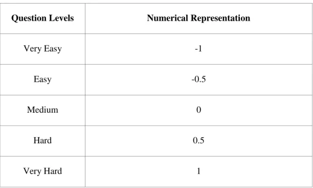
Table 3.2: Numerical Representations of Nominal Question Levels

Question Levels Numerical Representation

Very Easy -1

Easy -0.5

Medium 0

Hard 0.5

(25)

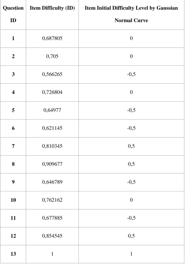
Table 3.3: Item Difficulty versus initial classes

Question ID

Item Difficulty (ID) Item Initial Difficulty Level by Gaussian Normal Curve 1 0,687805 0 2 0,705 0 3 0,566265 -0,5 4 0,726804 0 5 0,64977 -0,5 6 0,621145 -0,5 7 0,810345 0,5 8 0,909677 0,5 9 0,646789 -0,5 10 0,762162 0 11 0,677885 -0,5 12 0,854545 0,5 13 1 1

(26)

As seen above, there is no question in Class -1. This is something related to Gaussian Normal Distribution. Therefore, it can be declared that there are 4 classes of questions in Gaussian Normal Curve. What will be done is that this type of classification will be taught to software by ANN, SVM and ANFIS. Firstly, system will be trained with a training set of data classifed according to above classifcation and then expect them to predict latter set of data called test data properly.

3.4. CLASSIFICATION BY ANN

Three techniques were used to classify 13 questions into 4 categories. First technique that has been used to classify was ANN (Artificial Neural Network).

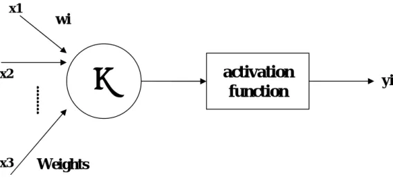
ANN is mostly used technique that is used in artificial intelligence related works. It uses such a neuron model that is the most basic component of a neural network. It is so important in classification as well. It is used to distinguish multiple broad classes of models. Figure 1 shows an example of a simplified neuron model (Haykin,1999). The neuron takes a set of input values, xi each of which is

multiplied by a weighting factor, wi . All of the weighted input signals are added

up to produce n, the net input to the neuron (Haykin,1999). An activation function, F, transforms the net input of the neuron into an output signal which is transmitted to other neurons.

(27)

Figure 3.1: Simplified Neuron Model (Haykin,1999)

Three inputs were used as follows: • Item Difficulty

• Item Response

• Initial Gaussian Item Level

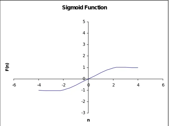
And it’s been tried to compute what question belongs to what class of Gaussian Normal Curve. Sigmoid function (tanh) was used as an activation function in regarding research because it works in the domain range between -1 and 1 that is the domain borders of our inputs (Haykin,1999). The sigmoid function is described by the following equation:

n

e

n

F

₋

+

=

1

1 )

(

(3.2) x3 x2 x1

Weights

...

..

.

activation

function

wi

yi

(28)

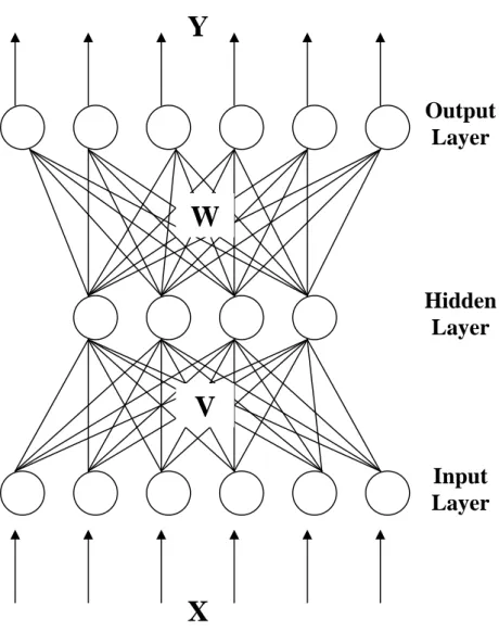
Figure 3.3 shows the sigmoid activation function. There are two important properties of sigmoid function which should be noted. The first one is that the function is highly non-linear. For large values of activation, the output of the neuron is restricted by the activation function. The second important feature is that the sigmoid function is continuous and continuously differentiable. Both this feature and the non-linearity feature have important implications in the network learning procedure (Haykin,1999). The basic structure of a feed forward neural network model is as follows:

Figure 3.2: Basic Structure of Feed Forward Network (Haykin,1999)

X

Y

W

V

Output

Layer

Hidden

Layer

Input

Layer

(29)

This neural network type that is multilayer feedforward neural network distinguishes itself by the presence of one or more hidden layers, whose computation nodes are correspondingly called as hidden neurons or hidden units. The function of hidden neurons is to intervene between the external input and the network output in some useful manner (Haykin,1999). By adding one or more hidden layers, the network is enabled to extract higher order statistics. In a rather loose sense the network acquires a global perspective despite its local connectivity due to the extra set of synaptic connections and the extra dimension of neural interactions. (Churchland and Sejnowski, 1992). The ability of hidden neurons to extract higher-order statistics is particularly valuable when the size of the input layer is large (Haykin,1999). Learning happens depending on the activation function as well. Sigmoid function was used and here is the graph of a sigmoid function sample as follows:

(30)

Sigmoid Function -3 -2 -1 0 1 2 3 4 5 -6 -4 -2 0 2 4 6 n F (n )

Figure 3.3: Sigmoid Function (Haykin,1999)

And here are the parameters that ANN used in regarding research as follows: • Percentage of Data in Training Part: 50%

• Percentage of Data in Validation Part: 25% • Percentage of Data in Testing Part: 25% • Number of Inputs: 3

• Number of Patterns: 13 • Num of Hidden Layers: 4 • Number of Epochs: 500

After executing the ANN filter, 4 classes of questions were obtained. In other words, ANN found the correct classes of Gaussian Normal Curve. Because Gaussian Normal Curve classified questions into 4 classes, ANN yielded 4

(31)

classes. This means that ANN learned Gaussian Normal Curve classification logic correctly.

3.5. CLASSIFICATION BY SVM

The second technique that was used for classification was SVM (Support Vector Machine). Same inputs of ANN and same percentages of data for training, validation and testing were used, however; SVM was not better than ANN in classification. Results will be evaluated in further sections of this thesis.

SUPPORT VECTOR machines (SVMs) (Genov, 2003 ; Boser, Guyon & Vapnik, 1992) offer a principled approach to machine learning combining many of the advantages of artificial intelligence and neural-network approaches. Underlying the success of SVMs are mathematical foundations of statistical learning theory (Genov, 2003 ; Vapnik, 1995). Rather than minimizing training error (empirical risk), SVMs minimize structural risk which expresses an upper bound on the generalization error, i.e., the probability of erroneous classification on yet-to-be-seen examples.

From a machine learning theoretical perspective (Genov, 2003 ; Vapnik, 1995), the appealing characteristics of SVMs are as follows:

(32)

• The learning technique generalizes well even with relatively few data points in the training set, and bounds on the generalization error can be directly estimated from the training data.

• The only parameter that needs tuning is a penalty term for misclassification which acts as a regularizer (Genov, 2003 ; Girosi, Jones & Poggio,1995) and determines a tradeoff between resolution and generalization performance (Genov, 2003 ; Pontil & Verri, 1998).

• The algorithm finds, under general conditions, a unique separating decision surface that maximizes the margin of the classified training data for best out-of-sample performance.

SVMs express the classification or regression output in terms of a linear combination of examples in the training data, in which only a fraction of the data points, called “support vectors,” have nonzero coefficients. The support vectors thus capture all the relevant data contained in the training set. In its basic form, a SVM classifies a pattern vector X into class y {-1,1} based on the support vectors Xm and corresponding classes ym as:

) ) , ( ( 1 b X X K sign y m m M m m

y

− =

∑

=

α

(3.3)

(33)

where K(.,.) is a symmetric positive-definite kernel function which can be freely chosen subject to fairly mild constraints (Genov, 2003 ; Boser, Guyon, Vapnik, 1992). The parameters and are determined by a linearly constrained quadratic programming (QP) problem (Genov, 2003 ; Vapnik, 1995 ; Burges,1998), which can be efficiently implemented by means of a sequence of smaller scale, subproblem optimizations (Genov, 2003), (Osuna, Freund, Girosi, 1997), or an incremental scheme that adjusts the solution one training point at a time (Genov, 2003 ; Cauwenberghs, Poggio, 2001). Most of the training data Xm have zero coefficients ; the nonzero coefficients returned by the constrained QP optimization define the support vector set. In what follows we assume that the set of support vectors and coefficients are given, and we concentrate on efficient run-time implementation of the classifier.

Several widely used classifier architectures reduce to special valid forms of kernels K(.,.),like polynomial classifiers, multilayer perceptrons,1 and radial basis functions (Genov, 2003 ; Schölkopf, et al. , 1997). The following forms are frequently used:

1) inner-product based kernels (e.g., polynomial; sigmoidal connectionist):

) ( ) . ( ) , ( 1

X

n N n mn m m f X X f X X K

∑

= = = (3.4)

(34)

2) radial basis functions (L2 norm distance based) ) ) | | (( ||) (|| ) , ( 2 / 1 2 1 n N n mn m m X X f X X f X X K − = − =

∑

= (3.5)

where f(.) is a monotonically nondecreasing scalar function subject to the Mercer condition on K(.,.) (Genov, 2003 ; Vapnik, 1995 ; Girosi, Jones & Poggio, 1995).

With no loss of generality, we concentrate on kernels of the inner product type (4), and devise an efficient scheme of computing a large number of high-dimensional inner-products in parallel.

Computationally, the inner-products comprise the most intensive part in evaluating kernels of both types (4) and (5). Indeed, radial basis functions (5) can be expressed in inner-product form as:

) ) || || || || . 2 (( ||) (|| X X f X X X 2 x 2 1/2 f m − = − m + m + (3.6)

Radial basis function was used in SVM and here are the statistical parameters and outputs of SVM in regarding research as follows:

• Percentage of Data in Training Part: 50% • Percentage of Data in Validation Part: 25%

(35)

• Percentage of Data in Testing Part: 25% • Average loss: 0.022227167

• Avg. loss positive: 0.0070014833 (965 occurences) • Avg. loss negative: 0.073067253 (289 occurences) • Mean absolute error: 0.022227167

• Mean squared error: 0.0033937631

SVM classified 13 questions into 4 categories as ANN did as well. However, ANN was better for learning of Gaussian Normal Curve Distribution.

3.6. CLASSIFICATION BY ANFIS

Finally, ANFIS method was used for classification of 13 questions. the same inputs were used and same classes of questions were obtained. However, performance was really great. ANFIS learned Gaussian Normal Curve Distribution very well and was the best among other two techniques: ANN and SVM. In order to understand why ANFIS was the best, the logic of ANFIS should be known firstly.

A Fuzzy Logic System (FLS) can be seen as a non-linear mapping from the input space to the output space. The mapping mechanism is based on the conversion of inputs from numerical domain to fuzzy domain with the use of fuzzy sets and fuzzifiers, and then applying fuzzy rules and fuzzy inference engine to perform

(36)

the necessary operations in the fuzzy domain (Estevez, Held U & Perez, 2006 ; Jang,1992).

The result is transformed back to the arithmetical domain using defuzzifiers. In this thesis, Adaptive Neuro-fuzzy Inference System (ANFIS) structure and optimization processes are used. The ANFIS approach uses Gaussian functions for fuzzy sets and linear functions for the rule outputs. The parameters of the network are the mean and standard deviation of the membership functions (antecedent parameters) and the coefficients of the output linear functions (consequent parameters).

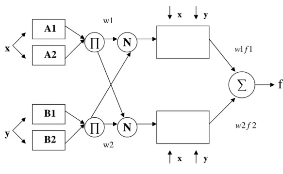
Figure 3.4: Anfis Architecture

The ANFIS learning algorithm is used to obtain these parameters. This learning algorithm is a hybrid algorithm consisting of the gradient descent and the least-squares estimate. Using this hybrid algorithm, the rule parameters are recursively updated until an acceptable error is reached. Iterations have two steps, one

x

y

A1

A2

B1

B2

N

x y y x w1 w2 1 1 f w 2 2 f w

f

(37)

fixed, and the consequent parameters are obtained using the linear least-squares estimate. In the backward pass, the consequent parameters are fixed, and the output error is back-propagated through this network, and the antecedent parameters are accordingly updated using the gradient descent method.

Takagi and Sugeno’s fuzzy if-then rules are used in the model. The output of each rule is a linear combination of input variables and a constant term. The final output is the weighted average of each rule’s output. The basic learning rule of the proposed network is based on the gradient descent and the chain rule (Riverol & Sanctis,2005).

In the designing of ANFIS model, the number of membership functions, the number of fuzzy rules, and the number of training epochs are important factors to be considered. If they were not selected appropriately, the system will over-fit the data or will not be able to fit the data. Adjusting mechanism works using a hybrid algorithm combining the least squares method and the gradient descent method with a mean square error method.

The aim of the training process is to minimize the training error between the ANFIS output and the actual objective. This allows a fuzzy system to train its features from the data it observes, and implements these features in the system rules.

(38)

As a Type III Fuzzy Control System, ANFIS has the following layers as represented in Fig. 5. The brief explanation of these layers and functions used within each layer is as follows;

Layer 0: It consists of plain input variable set.

Layer 1: Every node in this layer is a square node with a node function as

seen on Equation 5; i i b i i A

a

c

x























 −

+

=

2

1

1 )

(

µ

(3.7)

where A is a generalized bell fuzzy set defined by the parameters {a,b,c} , where c is the middle point, b is the slope and a is the deviation.

Layer 2: The function is a T-norm operator that performs the firing strength of the

rule, e.g., fuzzy AND and OR. The simplest implementation just calculates the product of all incoming signals.

Layer 3: Every node in this layer is fixed and determines a normalized firing

(39)

Layer 4: The nodes in this layer are adaptive and are connected with the input

nodes (of layer 0) and the preceding node of layer 3. The result is the weighted output of the rule j.

Layer 5: This layer consists of one single node which computes the overall output

as the summation of all incoming signals.

The model was used in regarding research for question classification. As mentioned before, according to the feature extraction process, 3 inputs are fed into ANFIS model and one variable output is obtained at the end. The last node (rightmost one) calculates the summation of all outputs (Jang,1993).

And here are the parameters that were used in ANFIS as follows: • Percentage of Data in Training Part: 50%

• Percentage of Data in Validation Part: 25% • Percentage of Data in Testing Part: 25% • Type of Fuzzy System: TSK

• Dimensions of the fuzzy system: • Number of Inputs: 2

• Number of Rules: 9 • Number of Outputs: 1

• A TSK system has only fuzzy sets for the inputs. • Fuzzy system type: TSK by ANFIS.

• Number of fuzzy sets for input variables: 7 • Number of fuzzy sets for output variables: 7

(40)

• I used Gaussian form of fuzzy sets for input and output variables.

• Initialization for output parameters of a TSK fuzzy system, the coefficients are randomly chosen from [-0.01,+0.01].

• In order to set all learning rates to an identical value, I used the sigma command as sigma 0,01.

(41)

4. TEST RESULTS

So far, three favourite artificial intellegence methods: ANN, SVM, and ANFIS are proposed as a means to achieve accurate question level diagnosis, intelligent question for E-Learning or distance education platforms.

In order to observe their question classification abilities depending on the item responses of students, item difficulties of questions and question levels that are determined by putting the item difficulties to Gaussian Normal Curve, the effectivenesses of ANN, SVM and ANFIS methods were evaluated by comparing the performances and class correctnesses of the sample questions (n=13) using the same 3 inputs as: item responses, item difficulties, question levels to 5018 rows of data that are the item responses of students in a test composed of 13 questions.

What has been done up to here is that we put the inputs to filters. At first, inputs were as follows:

Inputs that entered to ANN, SVM and ANFIS commonly:

• Item Difficulty • Item Response

• Initial Gaussian Item Level

Those inputs were put into three filters one by one and outputs were yielded as follows shown below:

(42)

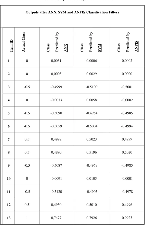
Table 4.1: Outputs of ANN, SVM and ANFIS

Outputs after ANN, SVM and ANFIS Classification Filters

It em I D A ct u a l C la ss C la ss P re d ic te d b y A N N C la ss P re d ic te d b y S V M C la ss P re d ic te d b y A N F IS 1 0 0,0031 0.0006 0,0002 2 0 0,0003 0.0029 0,0000 3 -0.5 -0,4999 -0.5100 -0,5001 4 0 -0,0033 0.0058 -0,0002 5 -0.5 -0,5090 -0.4954 -0,4985 6 -0.5 -0,5059 -0.5004 -0,4994 7 0.5 0,4998 0.5023 0,4999 8 0.5 0,4890 0.5196 0,5020 9 -0.5 -0,5087 -0.4959 -0,4985 10 0 -0,0091 0.0105 -0,0001 11 -0.5 -0,5120 -0.4905 -0,4978 12 0.5 0,4950 0.5010 0,4996 13 1 0,7477 0.7926 0,9923

(43)

If actual class values and predicted class values are benchmarked with respect to correctness parameter, following results are obtained. However, while calculating correctness values, all 13 questions were taken into account and average correctness values of 13 questions were obtained as in the table below.

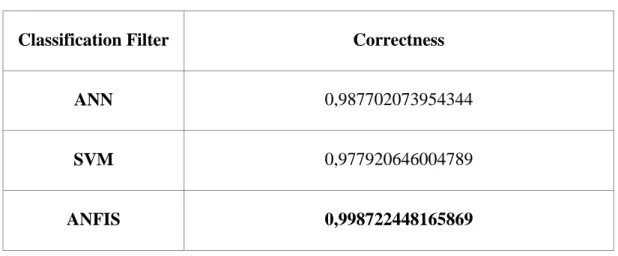
Table 4.2: Correctnesses of ANN, SVM and ANFIS

Classification Filter Correctness

ANN 0,987702073954344

SVM 0,977920646004789

ANFIS 0,998722448165869

As seen above, ANFIS found the best results and predicted the nearest values with respect to actual class values. In order to understand how ANN, SVM and ANFIS classified 13 number of questions with respect to what rule, the Gaussian Normal Curve logic have to be known and it must be seen that system learned Gaussian Normal Distribution at the training parts of 3 methodologies. What the Gaussian Normal Distribution is that the normal distribution, also called the Gaussian distribution, is an important family of continuous probability distributions, applicable in many fields. Each member of the family may be defined by two parameters, location and scale: the me

It is often called as bell curve because the graph of its probability density resembles a bell. In addition, the normal distribution maximizes information entropy among all distributions with known mean and

(44)

variance, which makes it the natural choice of underlying distribution for data summarized in terms of sample mean and variance. The normal distribution is the most widely used family of distributions in statistics and many statistical tests are based on the assumption of normality. In probability theory, normal distributions arise as the limiting distributions of several continuous and discrete families of distributions. This means that the area under the Gaussian curve is 1; that is the integration of Gaussian Curve function. From this probabilistic approach, normal distribution is used at classification as well. In this thesis, classification was done with respect to normal distribution and this provided equal deviations from the mean of class values. Gaussian Normal Curve and the class values is shown as seen below:

(45)

CLASS VALUES PREDICTED BY ANN,SVM and ANFIS -0,6 -0,4 -0,2 0 0,2 0,4 0,6 0,8 1 1,2 0 2 4 6 8 10 12 14 Question ID [1,13] C la s s V a lu e [ -1 ,1 ]

Actual Class Class Predicted by ANN Class Predicted by SVM Class Predicted by ANFIS

Figure 4.1: Class Values in Gaussian Curve

4.1. ERROR RATES OF CLASSIFICATION METHODS

As it is known that supervised learning is a machine learning technique for creating a function from training data and in artificial intelligence (AI) concept, an error rating table is an indicator that is generally used in supervised learning. Each column of the table represents the classifier filter instance, while each row represents the error rates in a predicted class. It is beneficial for benchmarking multiple classes in a system. In fact, an error rating table contains information about actual and predicted class values done by a classification system.

(46)

Table 4.3: Error Rates of Classification Methods

ANN SVM ANFIS

Error Rates Error Rates Error Rates

-1 0 0 0

-0,5 0,0142 0,00312 0,00228

0 0,00395 0,00495 0,000125

0,5 0,0108 0,01526667 0,001

1 0,2523 0,2074 0,0077

As seen above in the error rating table, the class named -1 has no error rates in all three ANN, SVM and ANFIS classifier because all three filters couldn’t find any class of data in the domain of -1. At first, according to Gaussian Normal Curve, system learned the classifying system and there were no class as -1. Therefore, all error rates in class -1 are zero above. The other indicators show that ANFIS has the least amount of error in classification depending on the error rates shown above.

4.2. RELATIVE IMAGINARY CLASSIFICATION RESULTS

DEPENDING ON THE ERROR RATES

In previous section, the error rates of classifiers were found and now it is the time to find how much data were classified correctly and wrongly. It will be more accurete to handle True and False classification results at each class done by three classifiers. Why this methodology is needed is that confusion matrices are

(47)

difficult or meaningless to use because classification results are so close to eachother, therefore, it has been planned to show the classification accuracies by giving relative values depending on the error rates handled in previous section and the number of rows of data the system includes at first. The relative imaginary classification results depending on the error rates are as follows shown below:

Table 4.4: Error Rates in Prediction

ANN SVM ANFIS T F T F T F -1 0 0 0 0 0 0 -0,5 1902,594 27,406 1923,978 6,0216 1925,599 4,400 0 1537,901 6,0988 1536,357 7,6428 1543,807 0,193 0,5 1145,494 12,506 1140,321 17,678 1156,842 1,158 1 288,6122 97,387 305,9436 80,056 383,0278 2,972

Since the classification results are so close to eachother, confusion matrices were not used to check the classifiers. Instead, the table above relatively shows the Accuracy, True-Positive, False-Positive, True-Negative, False-Negative and Precision values by relative imaginary true and false classification results. Again, it is seen that in all classes, ANFIS has the greatest deal of True Findings and the least amount of wrong matching with actual classes.

(48)

4.3. RECEIVER OPERATING CHARACTERISTIC CURVE ANALYSIS

ROC graphs are another way in addition to confusion matrices to analyze the performance of classifiers. A ROC graph is a plot with the false positive rate on the X axis and the true positive rate on the Y axis. The point (0,1) is the perfect classifier because it classifies all positive cases and negative cases correctly. It is (0,1) because the false positive rate is 0 (none), and the true positive rate is 1 (all). The point (0,0) represents a classifier that predicts all cases to be negative, while the point (1,1) corresponds to a classifier that predicts every case to be positive. Point (1,0) is the classifier that is incorrect for all classifications.

In many cases, a classifier has a parameter that can be adjusted to increase TP at the cost of an increased FP or decrease FP at the cost of a decrease in TP. Each parameter setting provides a (FP, TP) pair and a series of such pairs can be used to plot an ROC curve. A non-parametric classifier is represented by a single ROC point, corresponding to its (FP,TP) pair. A ROC Curve yields also a rate between TP and FP. The rate of approaching the point (1,1) yields the performance of classification system. This means that, the more graph approaches to point (1,1) rapidly, the more system is successful in classification. In the following pages, ROC Curves of ANN, SVM and ANFIS will be indicated and performance analysis will be done as well.

(49)

4.3.1. ROC Curve Analysis (ANN)

ROC Curve Analysis will be done depending on such parameters listed below:

TPR and FPR: True-Positive Rate and False-Positive Rate are the two axis: x

and y; that are the actual class and the predicted class representers. Those terms are also used in confusion matrix terminology and it is so beneficial to learn them before analyzing the ROC Curve in latter sections. Firstly; as it is known that supervised learning is a machine learning technique for creating a function from training data and in artificial intelligence (AI) concept, a confusion matrix is an indicator that is generally used in supervised learning. Each column of the matrix represents the instances in a predicted class, while each row represents the instances in an actual class. It is beneficial for benchmarking two classes in a system. In fact, a confusion matrix contains information about actual and predicted class values done by a classification system. Performance of such systems is commonly evaluated using the data in the matrix. The following table indicates the confusion matrix for a two class classifier.

• a is the number of correct predictions that an instance is negative,

• b is the number of incorrect predictions that an instance is positive,

• c is the number of incorrect of predictions that an instance negative,

• d is the number of correct predictions that an instance is positive.

Predicted

Negative Positive Negative a b Actual

(50)

By using this confusion matrix, several attributes are used to analyze the performance of classification. Those are as follows:

• Accuracy (AC) : is the proportion of the total number of predictions that

were correct. It is determined by using the equation:

d c b a d a AC + + + + = (4.1)

• True-Positive rate (TP) : is the proportion of positive cases that were

correctly identified, as calculated by using the equation:

d c d TP + = (4.2)

• False-Positive rate (FP) : is the proportion of negatives cases that were

incorrectly classified as positive, as calculated by using the equation:

b a b FP + = (4.3)

• True-Negative rate (TN) : is defined as the proportion of negatives cases

that were classified correctly, as calculated by using the equation:

b a a TN + = (4.4)

• False-Negative rate (FN) : is the proportion of positives cases that were

incorrectly classified as negative, as calculated by using the equation:

d c c FN + = (4.5)

(51)

• Precision (P) : is the proportion of the predicted positive cases that were

correct, as calculated by using the equation:

d b d P + = (4.6)

According to this terminology, ROC Curve uses these two parameters as its axises and the ROC Curve shows the relationship between TP and FP axises and this yields the performance and accuracy of classification.

AUC : is the abbreviation of ‘Area Under Curve’ and it is a so beneficial measure

of similarity between two classes measuring area under "Receiver Operating Characteristic" or ROC curve. In case of data with no ties all sections of ROC curve are either horizontal or vertical, in case of data with ties diagonal sections can also occur. AUC is always in between 0.5 and 1.0 values (Hand & Till, 2001).

SE(w): Standard error estimate under the area of ROC Curve. This shows the

average deviation from the findings of ROC resulting data.

Confidence Interval: The criterion commonly used to measure the ranking

quality of a classification algorithm is the area under the ROC curve (AUC). To handle it properly, it is important to determine an interval of confidence for its value. Confidence interval yields how the ROC curve is confidential with its results. Therefore, the higher confidence interval, the higher correctness in the results of classification.

(52)

Table 4.5: ROC Curve Analysis of ANN Class TPR FPR Area -1 1,0000 1,0000 ,0000 -0,5 1,0000 1,0000 ,3530 0 ,8089 ,6097 ,2485 0,5 ,7664 ,2942 ,1698 1 ,6791 ,0592 ,0201 AUC ,7914 SE(w) ,0227 Confidence Interval ,747 ,836

As seen in Table 4.5 above, classes with their TPR and FPR and the area under the each step of TP and FP axises are handled with software. Area means that at each step, the distance between ROC Curve point and the diagonal line changes depending on the values of TP and FP values. And also SE(w) that is standard error and the confidence error are the indicators of accuracy of classification. Necessary values to benchmark ANN with other filters are as follows with their values found by ANN below:

• AUC: 0,7914 • SE(w): 0,227

(53)

4.3.2. ROC Curve of ANN

AUC is the total area under the curve and it means that how much less amount of AUC exist, then, the classification is more accurate and has more performance. Therefore, in order to compare ANN with other filters, the parameter to be checked is AUC parameter. The less amount of AUC, the less amount of error in classification. AUC of ANN is 0,7914. Now, next step is to check SVM’s ROC Curve.

ROC Curve

,0 ,2 ,4 ,6 ,8 1,0 ,0 ,2 ,4 ,6 ,8 1,0

False Positive Rate

T

r

u

e

P

o

s

i

t

i

v

e

R

a

t

e

(54)

4.3.3. ROC Curve Analysis (SVM)

As seen in Table 4.6 below, classes with their TPR and FPR and the area under the each step of TP and FP axises are handled with software. Area means that at each step, the distance between ROC Curve point and the diagonal line changes depending on the values of TP and FP values. Necessary values to benchmark SVM with other filters are as follows with their values found by SVM below:

• AUC: 0,8748 • SE(w): 0,215

• Confidence Interval: 0,917

Table 4.6: ROC Curve Analysis of SVM

Class TPR FPR Area -1 1,0000 1,0000 ,0000 -0,5 1,0000 1,0000 ,3815 0 ,9459 ,6079 ,2855 0,5 ,8773 ,2948 ,1855 1 ,7186 ,0624 ,0224 AUC ,8748 SE(w) ,0215 Confidence Interval ,833 ,917

(55)

4.3.4. ROC Curve of SVM

AUC is the total area under the curve and it means that how much less amount of AUC exist, then, the classification is more accurate and has more performance. Therefore, in order to compare SVM with other filters, the parameter to be checked is AUC parameter. The less amount of AUC, the less amount of error in classification. AUC of SVM is 0,8748. This is greater than the ANN’s AUC and this means that ANN is better than SVM in classification. Now, next step is to check ANFIS’ ROC Curve.

ROC Curve

,0 ,2 ,4 ,6 ,8 1,0 ,0 ,2 ,4 ,6 ,8 1,0

False Positive Rate

T

r

u

e

P

o

s

i

t

i

v

e

R

a

t

e

(56)

4.3.5. ROC Curve Analysis (ANFIS)

As seen in Table 4.7 below, classes with their TPR and FPR and the area under the each step of TP and FP axises are handled with software. Area means that at each step, the distance between ROC Curve point and the diagonal line changes depending on the values of TP and FP values. Necessary values to benchmark ANFIS with other filters are as follows with their values found by ANFIS below:

• AUC: 0,5438 • SE(w): 0,1002

• Confidence Interval: 0,740

Table 4.7: ROC Curve Analysis of ANFIS

Class TPR FPR Area -1 1,0000 1,0000 ,0000 -0,5 1,0000 1,0000 ,2875 0 ,4956 ,6156 ,1493 0,5 ,4735 ,3074 ,0940 1 ,3407 ,0765 ,0130 AUC ,5438 SE(w) ,1002 Confidence Interval ,347 ,740

(57)

4.3.6. ROC Curve of ANFIS

AUC is the total area under the curve and it means that how much less amount of AUC exist, then, the classification is more accurate and has more performance. The less amount of AUC, the less amount of error in classification. AUC of ANFIS is 0,5438. This is the least amount of AUC and this means that ANFIS is the best classifier among other two other classifiers: ANN and SVM. Hence, ANFIS is better than ANN and ANN is better than SVM in classification.

ROC Curve

,0 ,2 ,4 ,6 ,8 1,0 ,0 ,2 ,4 ,6 ,8 1,0

False Positive Rate

T

r

u

e

P

o

s

i

t

i

v

e

R

a

t

e

(58)

5. DISCUSSIONS

As seen above, classification was done according to Gaussian Normal Curve and

ANFIS predicted the nearest class values. As seen on figures, all three filters drew

approximately the same parabola but there is a big difference at 13th question in prediction. ANFIS predicted it as 0,9923 while ANN predicted as 0,7477 and SVM predicted as 0,7926. ANN and SVM predicted approximately same but ANFIS found the nearest class value as 0,9923 while actual class value was 1. As it is seen in ROC Curves of ANN, SVM and ANFIS, it seems that the least error rates belong to ANFIS, and the most error rates belong to SVM. And also, if ROC Curves are analyzed one by one, it can be declared that ANFIS approaches to normal line that has angle of 45 with base faster than the others. ROC Curves shows at what rate each method approaches to correct classification. The closer path to normal line means that closer values predicted for classification and if a path drawn in ROC Curve comes closer to normal line and goes to the end point of normal line somehow finally, then; it means that that method has better performance, has better rate of finding true classification and has less amount of error of correctness in classification. ANFIS has the closest path to normal at overall and approaches to normal more quickly than the others. After ANFIS, if ROC Curves are analyzed again, ANN has a distance to normal line less than the SVM. The more drawn path gets far away from normal line, the least amount of correctness is yielded. Therefore, ANN is better than SVM. If we analyze all 3 methods with respect to the performance and correctness depending on the ROC Curves and other statistical data that mentioned before, it can be declared that

(59)

ANFIS is the best method among two others to classify the levels. Why ANFIS predicted the best class values is that ANFIS uses fuzzy-logic methodology while using ANN methodology additionally.

(60)

6. CONCLUSIONS AND FUTURE WORK

In this thesis, a classification model based on the three popular filter: ANN, SVM and ANFIS were proposed for the multiple choice question classification. Experiments were done in order to classify questions into 5 levels that are defined before entering filters by Gaussian Normal Curve. The effectivenesses of ANN, SVM and ANFIS methods were evaluated by comparing the performances and class correctnesses of the sample questions (n=13) using the same 3 inputs as: item responses, item difficulties, question levels to 5018 rows of data that are the item responses of students in a test composed of 13 questions. The comparative test performance analysis conducted using the classification correctness revealed that the Adaptive-Network-Based Fuzzy Inference System (ANFIS) yielded better performances than the Artificial Neural Network (ANN) and Support Vector Machine (SVM). This thesis provides an impetus for research on machine learning and artificial intelligence of question classification. Future research directions are as follows:

a) One of the shortcomings of the statistical method used in this project is that it

lacks semantic analysis. To strengthen the “semantic understanding” ability, the supplemental method, natural language processing such as expression normalization, and sentence understanding should be used during the text preprocessing. This requires the fact that questions will not be evaluated only with respect to their item difficulties and but also length of questions, the answer-question relation, similarity among answer-questions, semantic analysis etc.

(61)

b) To further test the effectiveness of the proposed model and to increase the

generality of the empirical study, more extensive experiments should be conducted by using larger training and test sets.

c) To find the most efficient classifier, additional machine learning or data mining

(62)

REFERENCES

Books

Haykin, S., 1999. Neural Networks: A Comprehensive Foundation, 2nd edn., Prentice Hall International, Inc.

Churchland P.S. and Sejnowski T.J., 1992. The Computational Brain, Cambridge, MA: MIT Press.

Periodical Publications

Genov R., Member, IEEE, and Gert Cauwenberghs, 2003. “Kerneltron:

Support Vector “Machine” in Silicon”, IEEE TRANSACTIONS ON

NEURAL NETWORKS, 14(5).

Jang J.- Jang S.R., 1992. “Self-learning fuzzy controllers based on temporal back propagation”, IEEE Trans. Neural Networks, 3(5), pp.714–723.

Jang J.- Jang S.R., 1993. “ANFIS: adaptive-network-based fuzzy inference system”, IEEE Trans. Syst. Man Cybernet, 23(3), pp.665–685.

Riverol C. and Di Sanctis C., 2005. “Improving Adaptive-network-based Fuzzy Inference Systems (ANFIS): A Practical Approach”, Asian Journal of Information Technology, 4(12), pp.1208-1212.

Schölkopf B., Sung K., Burges C., Girosi F., Niyogi P., Poggio T., and Vapnik V., 1997. “Comparing support vector machines with Gaussian kernels to radial basis functions classifiers,” IEEE Trans. Signal Processing, 45, pp. 2758–2765.

Vapnik V., 1995. The Nature of Statistical Learning Theory. New York: Springer-Verlag.

Intellegent question classification for e-learning environments by data mining techniques

INTELLIGENT QUESTION CLASSIFICATION FOR

E-LEARNING ENVIRONMENTS BY DATA MINING

TECHNIQUES

INTELLIGENT QUESTION CLASSIFICATION FOR

E-LEARNING ENVIRONMENTS BY DATA MINING

TECHNIQUES

ABSTRACT

ÖZET

TABLE OF CONTENTS

LIST OF TABLES

LIST OF FIGURES

LIST OF ABBREVIATIONS

1. INTRODUCTION AND PROBLEM DEFINITION

2. LITERATURE AND BACKGROUND

3. METHODOLOGIES

e

n

F

+

=

1

1

)

(

Weights

...

...

..

.

activation

function

wi

yi

X

Y

W

V

Output

Layer

Hidden

Layer

Input

Layer

y

∑

α

X

X

∑

∑

x

y

A1

A2

B1

B2

N

N

f

a

c

x

x



























 −

+

=