Informed feature regularization in voxelwise modeling for naturalistic fMRI experiments

3394

|

1

|

INTRODUCTION

Voxelwise modeling (VM) is a powerful framework to model single-voxel functional selectivity for the multi-tude of stimulus features that exist in natural stimuli (Kay, Naselaris, Prenger, & Gallant,  2008; Naselaris, Prenger, Kay, Oliver, & Gallant,  2009). Previous studies have

used this approach to sensitively model a broad range of representations from low-level spatiotemporal fea-tures to high-level object and action categories (Çukur, Nishimoto, Huth, & Gallant, 2013; Huth, Nishimoto, Vu, & Gallant,  2012; Lescroart, Stansbury, & Gallant,  2015; Nishimoto et al., 2011). In VM, an encoding model is con-structed that contains stimulus features hypothesized to

R E S E A R C H R E P O R T

Informed feature regularization in voxelwise modeling for

naturalistic fMRI experiments

Özgür Yılmaz

_|

_Emin Çelik

_|

_{Tolga Çukur}

© 2020 Federation of European Neuroscience Societies and John Wiley & Sons Ltd Edited by Christoph M. Michel

The peer review history for this article is available at https://publo ns.com/publo n/10.1111/ejn.14760

Abbreviations: BOLD, blood-oxygen-level-dependent; FI-VM, feature-informed voxelwise modeling; FMRI, functional magnetic resonance imaging;

JI-VM, jointly informed voxelwise modeling; ROI, region of interest; SI-VM, spatially informed voxelwise modeling; VM, voxelwise modeling. 1_{National Magnetic Resonance Research}

Center, Bilkent University, Ankara, Turkey 2_{Department of Electrical and Electronics} Engineering, Bilkent University, Ankara, Turkey

3_{Neuroscience Program, Sabuncu Brain} Research Center, Bilkent University, Ankara, Turkey

Correspondence

Tolga Çukur, Department of Electrical and Electronics Engineering, Bilkent University, Ankara TR-06800, Turkey.

Email: cukur@ee.bilkent.edu.tr

Funding information

National Eye Institute Grant, Grant/Award Number: EY019684; Marie Curie Action Career Integration Grant, Grant/Award Number: PCIG13-GA-2013-618101; European Molecular Biology Organization Installation Grant, Grant/Award Number: IG 3028; TUBA GEBIP 2015 fellowship; BAGEP 2017 fellowship; ASELSAN PhD scholarship; TUBITAK-BIDEB 2211 scholarship; NVIDIA GPU Grant

Abstract

Voxelwise modeling is a powerful framework to predict single-voxel functional se-lectivity for the stimulus features that exist in complex natural stimuli. Yet, because VM disregards potential correlations across stimulus features or neighboring voxels, it may yield suboptimal sensitivity in measuring functional selectivity in the presence of high levels of measurement noise. Here, we introduce a novel voxelwise modeling approach that simultaneously utilizes stimulus correlations in model features and response correlations among voxel neighborhoods. The proposed method performs feature and spatial regularization while still generating single-voxel response predic-tions. We demonstrated the performance of our approach on a functional magnetic resonance imaging dataset from a natural vision experiment. Compared to VM, the proposed method yields clear improvements in prediction performance, together with increased feature coherence and spatial coherence of voxelwise models. Overall, the proposed method can offer improved sensitivity in modeling of single voxels in natu-ralistic functional magnetic resonance imaging experiments.

K E Y W O R D S

elicit blood-oxygen-level-dependent (BOLD) responses in cortical voxels. For each voxel, a weighted linear combi-nation of model features that best explain measured BOLD responses is computed via regularized regression. To avoid over-fitting and ensure generalizability to new data, it is common to perform L2-norm regularization over model features with a uniform prior to penalize large model weights (Bishop,  2013). The regularization parameter is separately selected for each voxel based on a cross-valida-tion procedure. Following parameter seleccross-valida-tion, the result-ing model weights characterize the functional selectivity of single voxels.

Classical VM performs independent modeling to maxi-mize sensitivity to single voxels, yet it disregards potential response correlations among neighboring voxels across cortex (Erwin, Obermayer, & Schulten,  1995; Zarahn, Aguirre, & D’Esposito, 1997) as well as potential stimulus correlations among model features (Nunez-Elizalde, Huth, & Gallant, 2018). This in turn might reduce the sensitivity of VM in capturing functional selectivity in the presence of high levels of measurement noise. To better utilize response correlations, we recently proposed a spatial regularization term for VM via a graph Laplacian approach where neigh-borhoods were defined in volumetric brain space (Çelik, Dar, Yılmaz, Keleş, & Çukur,  2019). Spatially regularized VM models were found to improve model performance broadly across cerebral cortex. Yet, the proposed approach still uses L2-norm regularization over model features—a uniform Gaussian prior—that reflects the assumption that model features are uncorrelated (Hoerl & Kennard, 1970). This as-sumption might be suboptimal for models of natural stimuli. For example, in a category model that contains distinct ob-ject and action categories within natural scenes, the stimulus time courses for similar categories are correlated (e.g., “hu-man”-“hand,” “kid”-“run,” “building”-“road” and “park”-“tree”; Huth et  al.,  2012). Moreover, a voxel selective for humans will typically yield elevated responses to body parts, animate categories or human-related tools compared to unre-lated categories (Huth et al., 2012). As voxelwise functional selectivity profiles for related categories are expected to be similar, model weights are not truly uncorrelated (Nunez-Elizalde et al., 2018).

In this study, we propose a new VM approach to increase sensitivity in modeling functional selectivity (Figure  1). First, we introduce an informed feature regularization that takes into account correlations among model features. This is accomplished by enforcing similarity of model weights among features that are correlated to each other. To further boost model performance, we introduce a new spatial regu-larization term. We had previously proposed to define voxel neighborhoods based on Euclidean distances in volumetric brain space (Çelik et al., 2019). Yet, distances along the cor-tical surface are more likely to capture functional similarities

among neighboring voxels (Tucholka, Fritsch, Poline, & Thirion,  2012; Van Essen, Drury, Joshi, & Miller,  1998). Therefore, here we select voxel neighborhoods using geode-sic distances on the cortical surface. To achieve this goal, we measured intervoxel distances using inflated cortical spaces (Gao, Huth, Lescroart, & Gallant, 2015).

To independently evaluate improvements enabled by in-formed feature regularization and spatial regularization, we implemented three variants of VM together with Classical VM: a method that only uses informed feature regularization (feature-informed voxelwise modeling, FI-VM), a method that only uses spatial regularization (spatially informed vox-elwise modeling, SI-VM) and a method that simultaneously uses feature and spatial regularizations (jointly informed vox-elwise modeling, JI-VM). Demonstrations were performed on a category model fit to whole-brain BOLD responses re-corded while subjects watched natural movies. To measure correlations among 1,705 object and action category features in the model, we evaluated the pairwise similarities of the categories in a word embedding space obtained from a large text corpus. These similarities were then input to a graph Laplacian term, to form the feature and spatial regularization terms. The VM variants were compared in terms of their pre-diction scores and spatial and feature coherence of the result-ing model weights.

2

|

MATERIALS AND METHODS

2.1

|

MRI protocols

Magnetic resonance imaging (MRI) data were collected on a 3T Siemens Tim Trio scanner at the University of California, Berkeley, using a 32-channel Siemens volume coil. Functional scans were collected using a gradient EPI se-quence with repetition time = 2.00 s, echo time = 31 ms, flip angle = 70°, voxel size = 2.24 × 2.24 × 4.1 mm3_{, slice}

thick-ness = 3.5 mm with 18% slice gap, matrix size 100 × 100, and field of view = 224 × 224 mm2 _{and 32 axial slices.}

Anatomical data for three subjects were collected using a T1-weighted multi-echo MP-RAGE sequence on the same

3T scanner. Anatomical data for the other two subjects were collected on a 1.5T Philips Eclipse scanner.

2.2

|

Subjects

Functional data were collected from five healthy male subjects: S1 (age 25), S2 (age 25), S3 (age 25), S4 (age 32) and S5 (age 29). All subjects had normal or cor-rected-to-normal vision. The experimental protocol was approved by the Committee for the Protection of Human Subjects at the University of California, Berkeley. Prior

to scanning, written informed consent was obtained from all subjects.

2.3

|

Experimental procedure

The movie stimulus was identical to the set used in Nishimoto et al. (2011). The stimulus contained short clips (10–20 s) of color natural movies taken either from Apple QuickTime gallery (http://trail ers.apple.com/) or from YouTube (http:// www.youtu be.com/). The list of selected movies is as follows: “Artbeats HD,” “Australia,” “Bolt,” “BBC Motion Gallery,” “Bride Wars,” “Changeling,” “Duplicity,” “Fuel,” “Hotel for Dogs,” “IGN Game of the Year 2008,” “Ink Heart,” “JAL Boeing 747 landing Kai Tak,” “King Lines,” “Madagascar 2,” “Mall Cop,” “Mammoth HD,” “Pink Panther 2,” “Proud American,” “Role Models,” “Shark Water,” “Star Trek,” “The

American Recovery and Reinvestment Plan,” “The Macaulay Library,” “The Tale of Despereaux,” “Warren Miller Higher Ground,” “Where the hell is Matt?” and “Yes Man.” Original movie frames were cropped to square form and downsampled to 512 × 512 pixels. The stimulus was presented on 24°×24° degrees of visual angle. A fixation spot (0.16° square) was su-perimposed on the center of the screen and its color was al-ternated at 3 Hz, to make it continuously visible. For model estimation, 7,200 s (3,600 time samples, TR = 2 s) of mov-ies were presented to the subjects in 12 separate 10-min runs. For model validation, a different collection of 9 separate 1-min movie clips were selected. The selected clips were aggregated in randomized order to create in 9 separate 10-min runs. As such, each 1-min validation clip was presented to the subjects 10 times, and functional magnetic resonance imaging (fMRI) data were averaged across the 10 repeats to alleviate noise. These procedures resulted in 270 time samples of validation

FIGURE 1 Natural movie experiment and model fitting. (a) Whole-brain BOLD responses were acquired while subjects viewed natural movies. To estimate functional selectivity in single voxels, we fit voxelwise models that optimally predict measured BOLD responses in terms of the category features present in the movie stimuli (Huth et al., 2012). The resulting models describe how each of the 1,705 object and action categories in the movie stimulus evokes BOLD responses. (b) Classical voxelwise modeling (VM) ignores potential correlations in stimulus features and correlations among neighboring voxels. Feature-informed voxelwise modeling (FI-VM) takes into account correlations among model features to increase accuracy in predicting single-voxel selectivity. The resulting models have increased feature coherence. Jointly informed voxelwise modeling (JI-VM) further incorporates shared information between neighboring voxels. The resulting voxelwise models have both increased feature and spatial coherence [Colour figure can be viewed at wileyonlinelibrary.com]

data. To minimize the effects of hemodynamic transients, data obtained in the first 10 s of each run were omitted. Note that the same data were analyzed in several previous studies (Çelik et al., 2019; Çukur, Huth, Nishimoto, & Gallant, 2013; Çukur, Nishimoto, et al., 2013; Huth et al., 2012).

2.4

|

ROI abbreviations

Regions of interest (ROIs) used in our study are as follows: visual areas (V1–V4, V7), fusiform face area (FFA), extrastri-ate body area (EBA), occipital face area (OFA), parahippocam-pal place area (PPA), occipital place area (OPA), retrosplenial cortex (RSC), intraparietal sulcus (IPS), lateral occipital visual area (LO), frontal eye fields (FEF), supplementary eye fields (SEF), frontal operculum (FO), primary motor and somatosen-sory foot areas (M1F, S1F), primary motor and somatosensomatosen-sory hand areas (M1H, S1H), primary motor and somatosensory mouth areas (M1M, S1M), supplementary motor hand area (SMHA) and supplementary motor foot area (SMFA).

2.5

|

Functional localizers

For each subject, we defined boundaries of common functional ROIs by using three sets of functional localizers: a visual cat-egory localizer, a retinotopic localizer and a motor localizer.

In the visual category localizer, each subject was shown colored images of either places, faces, human body parts, animals, household objects or spatially scrambled household objects. The localization data were collected in 6 4.5-min runs. A single run consisted of 16 blocks, each 16 s long and separated with 500-ms interblock intervals. In each block, 20 images of either places, faces, human body parts, animals, household objects or spatially scrambled household objects were displayed. Each image was shown for 300 ms after a 500-ms interstimulus interval. Fusiform face area (FFA) and occipital face area (OFA) were defined using the faces ver-sus objects contrast (Kanwisher, McDermott, & Chun, 1997). Extrastriate body area (EBA) was defined using the human body parts versus objects contrast (Downing, Jiang, Shuman, & Kanwisher, 2001). Parahippocampal place area (PPA), ret-rosplenial cortex (RSC) and occipital place area (OPA) were defined using the scenes versus objects contrast (Epstein & Kanwisher, 1998; Nakamura, 2000).

Retinotopic mapping data were collected in four 9-min scans. The subjects were shown clockwise and counterclockwise rotat-ing wedges in two scans, expandrotat-ing and contractrotat-ing rrotat-ings in the remaining two scans. V1, V2, V3, V4, V7 and LO were defined based on visual angle and eccentricity maps. Using V1, V2 and V3, a broad retinotopic area (RET) was defined.

Motor localizer data were collected in a single 10-min scan. Each subject performed 6 separate motor tasks in random

blocks of 20 s. During the “hand” cue, the subject made small finger-drumming movements with both hands. During the “foot” cue, the subject made small toe movements. During the “mouth” cue, the subject made small mouth movements mimicking the syllable balabalabala. During the “speak” cue, the subject subvocalized self-generated sentences. During the “saccade” cue, the subject performed rapid saccades between different targets on the screen. During the “rest” cue, the sub-ject did not perform any motor tasks. Contrast between the “saccade” and “rest” conditions was used to define intraparietal sulcus (IPS), frontal operculum (FO), frontal eye fields (FEF) and supplementary eye fields (SEF). Contrast between “foot” and “rest” was used to define primary motor and somatosen-sory foot areas (M1F, S1F) and supplementary motor foot area (SMFA). Contrasts between “hand” and “rest” were used to define primary motor and somatosensory hand areas (M1H, S1H) and supplementary motor hand area (SMHA). Contrast between “mouth” and “rest” was used to define primary motor and somatosensory mouth areas (M1M, S1M). In this study, we aimed to examine how object and action features in natural movies modulate BOLD responses in single voxels. As it is commonly considered that motor and somatosensory areas do not play a major role in visual category representation, voxels within these regions were excluded from subsequent analyses.

2.6

|

Data preprocessing

Motion correction and image realignment were done using the Motion Correction FMRIB Linear Image Registration Tool (MCFLIRT) in FSL (Woolrich et al., 2009). Functional images of each subject were registered to a preselected image of that subject. The final time series data were manually checked for accuracy. The resulting time courses were z-scored individually for each voxel. No spatial smoothing was applied to the fMRI data.

Detrending was used to remove low-frequency drifts in BOLD responses. The drifts were estimated using a median filter with a 120-s window and then subtracted from mea-sured BOLD responses.

Brain Extraction Tool in FSL was used to eliminate non-cortical voxels. The set of voxels within a 4 mm radius of the cortical surface were defined as cortical voxels. Following analyses were done on a total of 35,158 ± 887 cortical voxels (mean ± SD across subjects).

2.7

|

Cortical flat maps

Cortical flat maps of subjects were generated using FreeSurfer (Dale, Fischl, & Sereno, 1999). These flat maps are based on T1-weighted anatomical scans. Anatomical

using Pycortex (Gao et al., 2015). Relaxation cuts were made into the surface of each hemisphere, and the surface crossing the corpus callosum was removed. The calcarine sulcus cut was made at the horizontal meridian in V1. Functional im-ages were aligned to the cortical flat maps using boundary-based registration (BBR) in FSL. For visualization of flat maps, the mid-cortical surface that lies halfway between the pial and white matter surfaces was selected.

2.8

|

Category model

To extract category information present in the natural movie stimulus, we used a category model (Çukur, Nishimoto, et al., 2013; Huth et al., 2012). We tagged object and action categories in each 1-s portion of the natural movies using the WordNet lexicon (Miller & Miller,  1995). Finally, a list of features including 1,705 distinct object and action categories was formed. Note that, the same list of object and action categories (1,705 features in total) was used in all four modeling methods. The time courses of the features were resampled using a 3-lobe Lanczos filter with a cutoff frequency of 0.249 Hz (the Nyquist frequency of the fMRI acquisition). To reduce dimensionality and improve model fits, we applied PCA onto the resulting stimulus matrix. We selected only the first 300 PCs that explain 89.2% of the variance in the stimulus. To rule out possible biases due to correlations between category model and global motion energy, we added a nuisance regressor that reflects the total motion energy in the movie stimulus. To obtain the total motion energy, we summed the output of all spatiotempo-ral Gabor filters used in a separate motion energy model (Çelik et al., 2019).

2.9

|

Voxelwise model

estimation and validation

We used a voxelwise modeling framework to fit between stimulus and BOLD responses (Çukur, Nishimoto, et al., 2013; Huth et al., 2012). In the Classical VM approach, L2

-regularized linear regression is used to predict how each feature modulates measured BOLD responses. A category model was fit to measure voxelwise selectivity for high-level object and action categories (Huth et al., 2012). To account for hemodynamic delays, a finite-impulse-response (FIR) fil-ter with three time delays (4, 6 and 8 s) was applied to each model feature before fitting the model.

where Y is the response matrix of size (number of TRs × num-ber of voxels), X is the stimulus matrix of size (numTRs × num-ber of

TRs × (3 × number of features)), and W is the weight matrix of size ((3 × number of features) × number of voxels). In VM, L2

-regularized regression is used to minimize the cost function:

where wi is the vector containing category model weights for

voxel-i, and yi is the vector containing the time course of BOLD

responses of voxel-i. Cost function can be expressed in matrix form as follows:

Data from single voxels were aggregated into matrix form to speed up computations. Note that the minimization was still performed for each voxel separately as each column of the weight matrix (W) is the vector containing category model weights for the corresponding voxel and the minimi-zation procedure does not involve any interaction among the columns. In Equation 3, by setting the gradient with respect to W to zero, we have:

To obtain model weights and to measure prediction scores, a 100-fold cross-validation was used. In each fold, a total of 3,600 samples were split into a contiguous block of 3,000 samples for model fitting and a remaining contiguous block of 600 test samples for selection of L2 regularization

parameter (λ). Separate models were fit for 30 different regu-larization parameters in the range of 10–2 _{to 10}7 _(spaced

log-arithmically). We calculated prediction scores based on the coefficient of determination (i.e., explained variance, R2₎

be-tween measured and predicted BOLD responses. Separately for each voxel, we picked the regularization parameter that maximized the average prediction score across folds. Final voxelwise models based on the optimal parameters were refit using the entire 3,600 time samples.

To measure final prediction scores, a 1,000-fold jackknife resampling at a rate of 80% was used on a separate validation data (270 samples). Separately for each voxel, final predic-tion score was taken as the average predicpredic-tion score across jackknife folds. For assessment of model performance, we then computed the average prediction score across five sub-jects in each functional ROI.

(1) X × W = Y (2) min w_i ∑ i‖‖Xwi−yi‖‖ 2 2+ 𝜆 ∑ i‖‖wi‖‖ 2 2 i=1, 2, …, Nvox (3) min w_i Tr [ (XW − Y)T (XW − Y)]+ 𝜆Tr(WTW) min w_i Tr ( WTXTXW)−2Tr(YTXW)+Tr(YTY)+ 𝜆Tr(WTW) i=1, 2, …, Nvox (4) 2XTXW − 2XTY + 2𝜆W = 0 XTXW + 𝜆W = XTY ( XTX + 𝜆I)W = XTY W =(XTX + 𝜆I)†XTY

2.10

|

Parameter optimization

In the proposed approach, there are five hyperparameters to be optimized. Three of these parameters (λ, λf and λs)

are set separately for individual voxels in each method. The remaining two hyperparameters (the standard devia-tion of Gaussian filter and the feature similarity threshold) determine the feature Laplacian matrix (F). The feature Laplacian matrix F is of size N_feat×N_feat, where N_feat is the

number of category features. F = T – S, where sjk (entries

of matrix S, see Equation 5) is the relatedness metric of the feature-j and feature-k (high for related features, and low or zero for distant features), and T is a diagonal matrix with

T_jj=∑_ks_jk.

sjk is calculated within a word embedding space

(Deerwester, Dumais, Furnas, Landauer, & Harshman, 1990; Lund & Burgess,  1996; Mitchell et  al.,  2008; Turney & Pantel,  2010; Wehbe et  al.,  2014). The word embedding space was formed based on word co-occurrence statistics. The assumption here is that words with similar meaning tend to occur in nearby positions in text. The co-occurrence sta-tistics were taken from a large corpus of text. This corpus contained words from transcripts of many popular books, Wikipedia pages and user comments gathered from reddit. com (604 popular books, 2,405,569 Wikipedia pages and 36,333,459 user comments scraped from reddit.com). In the corpus, 10,470 distinct words appeared 1,548,774,960 times (Huth, de Heer, Griffiths, Theunissen, & Gallant, 2016). Co-occurrences among the words from a lexicon of 10,470 words and the 985 basis words (from Wikipedia's List of 1,000 Basic Words) were calculated. The appearance of a lexicon word within a 15-word neighborhood of the basis word was taken as a single co-occurrence. We reduced the word em-bedding space by projecting onto the PC space obtained in Category Model. As a result, each of the 1,705 category fea-tures had a 300-dimensional vector representing its location in the reduced word embedding space. We then computed the similarity (cosine similarity, csjk) of each feature pair. We

eliminated feature pairs that have a similarity smaller than the feature similarity threshold (dsim). Later, we fed those

simi-larity values into a Gaussian filter, to get the final form of the relatedness metric (sjk) as in Equation 5.

Standard deviation (σ) and feature similarity threshold (dsim) were optimized a priori via a cross-validation

proce-dure on the training data. To do this, we computed voxelwise prediction scores of separate JI-VM models with standard de-viations of [0.1, 0.2, 0.4, 0.8, 1.2, 2.0] and feature similarity

thresholds of [0.1, 0.2, 0.3, 0.5]. The model with a standard deviation (σ) of 0.4 and a feature similarity threshold (dsim) of

0.2 outperformed others in most ROIs; thus, we fixed these parameters throughout our study.

To incorporate spatial regularization into VM, we con-structed a spatial Laplacian matrix that represents correlated information across neighboring voxels. The spatial Laplacian matrix (L) is of size N_vox×N_vox, where N_vox is the number

voxels in the subject. L = P – C, where cil (entries of

ma-trix C) corresponds to the proximity of voxel-i and voxel-l in three-dimensional space (high for immediate neighbors, and low or zero for voxels far away), and P is a diagonal matrix with P_ii=∑_lc_il. The weight c_il represents the cost of having

weights of voxel-i and voxel-l more dissimilar to each other. To compute cil, first the distance between voxel-i and voxel-l

is calculated as the Euclidean distance between those voxels in inflated cortical space (Gao et al., 2015). Calculated dis-tances are then input to a Gaussian filter. We have two hyper-parameters in constructing the spatial Laplacian matrix L: the proximity limit after which two voxels are treated as spatially uncorrelated and the standard deviation of the Gaussian filter. Here, we prescribed these hyperparameters reported by Çelik et al. (2019) by converting into millimeter scale to use in our approach.

The other three hyperparameters are regularization parame-ters of L2 regularization, feature regularization and spatial

reg-ularization: λ, λf and λs, respectively. λ indicates the degree of

L2 regularization across model features. λf indicates the degree

of penalization applied to the differences within the weights of related feature pairs. λs indicates the degree of spatial

regular-ization across category features of neighboring voxels. As vox-els across cortex may need varying degrees of regularization, we optimized these parameters separately for each voxel.

2.11

|

JI-VM model

estimation and validation

Cost function for the regularized regression in the proposed approach can be expressed as follows:

where the third term is the feature regularization term, and the last term is the spatial regularization term. In the feature regularization term, the weighted sum of Euclidean distances between each feature pair is calculated for each voxel sepa-rately. sjk represents the cost of having model weights for

fea-ture-j and feature-k dissimilar to each other (Equation 5). In the spatial regularization term, the weighted sum of Euclidean distances between weights of voxels is calculated. The weight cil represents the cost of having vectors containing category

(5) s_jk= ⎧ ⎪ ⎨ ⎪ ⎩ exp � −(1−cs_jk)2 2𝜎2 � , cs_jk≥d_sim 0, cs_jk<_d sim (6) min wi ∑ i‖‖Xwi−yi‖‖ 2 2+ 𝜆 ∑ i‖‖wi‖‖ 2 2+ 𝜆f ∑ i ∑ j,ksjk ( wij−wik )2 + 𝜆_s∑ i,lcil‖‖wi−wl‖‖ 2 2

model weights of voxel-i and voxel-l dissimilar to each other (see Section 2.10).

Cost function can be expressed in matrix form as follows:

Then, by setting the gradient with respect to weight matrix (W) to zero, we now have:

To simplify Equation 8, we define K = XT_X, _{M = X}T_Y and

B = 𝜆_sL:

2.12

|

Pseudo-code for JI-VM

implementation

Equation 9 cannot be solved with a single pseudo-inverse. An efficient algorithm for the solution from Çelik et al. (2019) is given in Table 1.

2.13

|

FI-VM and SI-VM model

estimation and validation

In FI-VM, we only include feature regularization term; there-fore, λs is set to 0 in Equation 8:

Solution to this equation is as follows:

As the solution can be expressed via a single pseudo-in-verse, we implemented the same cross-validation procedure as in Classical VM. This time, separate voxelwise models were fit for 30 × 30 different regularization parameter pairs (𝜆_{, 𝜆}

f), each in the range from 10–2 to 107 (spaced

logarith-mically). We measured the prediction scores using the same jackknife resampling method.

In SI-VM modeling, on the other hand, we removed the feature regularization term from JI-VM, equivalently setting

𝜆_f=0 in Equation 8:

The implementation for SI-VM is the same as JI-VM case with setting A = (K + 𝜆I) and omitting the second loop with λ_f

from pseudo-code (see Section 2.12).

(7) min w_i Tr [ (XW − Y)T(XW − Y)]+ 𝜆Tr(WTW)+ 𝜆_fTr(WTFW)+ 𝜆_sTr(WLWT) min w_i Tr ( WTXTXW)− 2Tr(YTXW)+Tr(YTY)+ 𝜆Tr(WTW)+ 𝜆_fTr(WTFW)+ 𝜆_sTr(WLWT)

for i=1,2,…,Nvox

(8) 2XTXW − 2XTY + 2𝜆W + 2𝜆fF T W + 2𝜆sWL = 0 XTXW + 𝜆W + 𝜆_fFTW + 𝜆_sWL = XTY ( XTX + 𝜆I + 𝜆fFT ) W + 𝜆sWL = XTY (9) ( K + 𝜆I + 𝜆fFT ) W + WB = M AW + WB = M (10) ( XT_{X + 𝜆I + 𝜆} fFT ) W = XT_Y (11) W =(XTX + 𝜆I + 𝜆_fFT)†XTY (12) ( XTX + 𝜆I)W + 𝜆_sWL = XTY

TABLE 1 Pseudo-code for JI-VM

Solve: (AW + WB = M) begin

for λ: for λf:

Find eigenvalues of A and store them in D

Set D₍ d  = diag(D), where Dd is a column vector of size

3 × Nfeat ) Set Dr= [ Dd, Dd, … ]

, where Dd repeats Nvox times; Dr is of

size (3 × Nfeat

) ×(Nvox

)

Find eigenvectors of A and store them in Q

for λs: Set Sr= [ Sd; Sd; … ]_{, where S} d repeats (3 × Nfeat ) _{times; S} r is of size (3 × Nfeat ) ×(Nvox ) P =1.∕(Dr+ 𝜆sSr )

, where P is of size (3 × Nfeat

) ×(Nvox

) W* = −Q(P.*(QT_MU))UT

Variables:

Input:X: stimulus matrix of size (time points) ×(3 × Nfeat

)

Y: response matrix of size (time points) ×(N_vox)

K: auto-covariance matrix of size (3 × Nfeat

) ×(3 × Nfeat

) , where K = XT_X

M: cross-covariance matrix of size (3 × Nfeat

) ×(Nvox

) , where

M = XT_Y

λ: regularization parameter for L2-norm regularization λf: regularization parameter for feature regularization

λs: regularization parameter for spatial regularization

A: auto-covariance matrix of size (3 × Nfeat

) ×(3 × Nfeat

) , where

A =(K + 𝜆I + 𝜆_fF)

F: Laplacian matrix of size (3 × Nfeat

) ×(3 × Nfeat

)

, which stores similarity information between category features

L: Laplacian matrix of size (Nvox

) ×(Nvox

)

, which stores proximity information between voxels

B: B = 𝜆sL

Output: W: model weight matrix of size (3 × Nfeat

) ×(Nvox

) Precompute Schur decomposition of L, L = USUT

Save U and Sd, where Sd = diag(S) is of size 1 ×(Nvox

2.14

|

Alternative voxelwise modeling

method: graph net regularization

As an alternative to Classical VM, voxelwise models were also fit using graph net regularization (Schoenmakers, Barth, Heskes, & van Gerven, 2013). Graph net regularization uti-lizes a coupling matrix to enforce similar model weights across related features. As such, the optimization objective for Graph-Net VM is given as follows:

Here, G is a non-diagonal matrix that induces coupling between model features (Grosenick, Klingenberg, Katovich, Knutson, & Taylor, 2013; Schoenmakers et al., 2013). Gjk equals −1 when

two features (feature-j and feature-k) are coupled, 0 otherwise, and Gii equals the number of features that feature-j is coupled

to. For the category features examined in this study, Gjk is set to

−1 when the two features are semantically related (i.e., s_jk>₀,

see Section 2.10), 0 otherwise (s_jk=0). Note that, unlike our

proposed feature regularization method, the degree of semantic similarity is binary-valued in Graph-Net VM.

Solution to Equation 13 is computed as a single pseudo-inverse:

Graph-Net VM was implemented via the same procedure as in Classical VM (100-fold cross-validation, the hyperpa-rameter λ was selected from 30 values in the range from 10–2

to 107_{). Prediction scores were computed based on the}

coeffi-cient of determination (explained variance, R2_{) between}

mea-sured and predicted BOLD responses. To measure prediction scores, a 1,000-fold jackknife resampling at a rate of 80% was used on a separate validation data (270 samples). Separately for each voxel, final prediction score was taken as the average prediction score across jackknife folds.

2.15

|

Feature coherence analysis

We hypothesized that the human brain encodes information in a way where related features elicit similar responses in single voxels (Huth et al., 2012). In the VM framework, this hypoth-esis would manifest itself as coherent model weights across related features for individual voxels. Because Classical VM ignores feature correlations, it can have reduced sensitivity in capturing coherence among model features. Yet, informed feature regularization enforces increased coherence among category features. Thus, in FI-VM and in JI-VM, resulting model weights are expected to be more coherent. To test this hypothesis, we defined a voxelwise feature coherence metric.

We computed the contribution of voxel-i to the feature regu-larization cost in the regression analysis:

where the differences between weights of correlated fea-tures (i.e., for pairs of [feature-j, feature-k] where sjk > 0, see

Equation 5) are penalized according to a graph Laplacian matrix computed in the word embedding space (fjk are the entries of the

Laplacian matrix F corresponding to feature-j and feature-k, see Section 2.10). Voxelwise cost values were then normalized with the maximum cost obtained across the three methods (FI-, SI- and JI-VM). The normalized cost was inverted to finally obtain the feature coherence metric.

2.16

|

Spatial coherence analysis

Human brain encodes information across spatial clusters of neural populations (Engel, Glover, & Wandell, 1997; Huth et al., 2012; Tootell et al., 1998). Thus, it is expected that neighboring voxels represent correlated information. As Classical VM ignores spatial correlations among neighbor-ing voxels, it is expected to fail in capturneighbor-ing the coherence in neighboring voxels. Due to spatial regularization, the proposed approach should be more sensitive in capturing the spatial coherence. To test this prediction, we computed a voxelwise spatial coherence metric. The spatial coherence of voxel-i was taken as the mean standard deviation among category model weights of the voxels within close spatial proximity of voxel-i (i.e., for any voxel-l where c_il>₀, see

Section 2.11):

We normalized those values by dividing by the largest value computed across the three methods and then inverting the resulting value to obtain the final form of the spatial co-herence metric.

2.17

|

Noise ceiling

The coefficient of determination (R2_{) between predicted}

response and measured response can be biased downward due to high measurement noise in voxel responses (David & Gallant,  2005; Hsu, Borst, & Theunissen,  2004; Sahani & Linden, 2003). As validation data were recorded a finite number of repeats (10 in this study), it is likely to contain high measurement noise in addition to signal. We calculated a noise ceiling for each voxel following procedures in Hsu et al. (Hsu et al., 2004). A voxelwise correction factor was (13) min w_i ∑ i‖‖Xwi−yi‖‖ 2 2+ 𝜆 (∑ iw T iGwi ) (14) W =(XTX + 𝜆G)†XTY (15) 𝜎i feature= ∑ j,kfjk ( w_ij−w_ik)2 (16) 𝜎i spatial= ∑ icil‖‖wi−wl‖‖ 2 2

calculated by dividing the maximum possible prediction score (called the noise ceiling) by the raw prediction score of each voxel. For voxels with very high level of noise, this process leads to divergent correction factors. We limited cor-rection factors of these voxels to the average of corcor-rection factors across remaining cortical voxels.

2.18

|

Statistical analysis

Models were compared in terms of prediction score, feature coherence and spatial coherence. Specifically, changes in prediction score or coherence were calculated for various modeling methods over Classical VM. A bootstrap procedure with 10,000 samples was used to test significant changes in a given metric (prediction score or coherence) in each ROI. The null distribution was estimated via bootstrap sampling on metric values of Classical VM. The significance threshold was taken as the 95th percentile of the null distribution for each metric (α = 0.05).

3

|

RESULTS

3.1

|

Prediction scores of VM methods

The proposed method employs additional regulariza-tion terms to consider correlaregulariza-tions among model features as well as response correlations among voxel neighbor-hoods. As such, the fit models are expected to better cap-ture voxelwise functional selectivity than Classical VM. As an alternative to Classical VM, we have also imple-mented Graph-Net VM (see Section 2.14, Schoenmakers et al., 2013). Yet, no significant difference was observed between Graph-Net VM and Classical VM in many regions of interest (ROIs, see Sections 2.4 and 2.5; Figure S1). Thus, subsequent comparisons were provided against Classical VM as the reference method. To examine the contributions of the individual regularization terms, we separately com-puted improvements in prediction scores of FI-VM, SI-VM and JI-VM over Classical VM (see Section 2.9 for calcula-tion of prediccalcula-tion score). Figure 2 displays the change in explained variance for FI-VM, SI-VM and JI-VM in com-mon functional ROIs. We find that FI-VM significantly improves prediction scores compared to Classical VM in all of the examined ROIs except FFA, OFA and OPA (p < .05, bootstrap test). The average improvement in pre-diction scores is 0.020 ± 0.004 (ΔR2_{, mean ± SD across}

ROIs) for category-selective areas (FFA, PPA, EBA, OFA and OPA), 0.017 ± 0.003 for attention control areas (IPS, FEF, SEF and FO) and 0.008 ± 0.001 for early visual areas (RET, V4). These results suggest that informed feature regularization particularly improves model accuracy in

category-selective areas. These results can be attributed to the fact that representations in category-selective areas are mediated by object and action category features, whereas those in early visual areas are mediated primarily by reti-notopic features (Connolly et  al.,  2012; Downing, Chan, Peelen, Dodds, & Kanwisher,  2006; Engel et  al.,  1997; Huth et  al.,  2012; Naselaris et  al.,  2009; Op De Beeck, Haushofer, & Kanwisher, 2008; Tootell et al., 1998).

We also find that SI-VM significantly improves prediction scores in all ROIs except for FFA, OPA and RSC (p < .05, bootstrap test). These improvements are substantial broadly across cortex (0.039  ±  0.007 for category-selective areas, 0.022 ± 0.003 for attention control areas and 0.016 ± 0.002 for early visual areas). This result implies that spatial cor-relations among voxel neighborhoods exist across multiple

FIGURE 2 Improvement in prediction performance over VM by FI-VM, SI-VM and JI-VM. The improvement in prediction performances for the three methods (FI-, SI- and JI-VM, see Abbreviations) over VM is shown for several well-known functional ROIs (see Abbreviations). Bar graphs display improvement in prediction scores (ΔR2_{, mean ± SD across subjects, see Section 2.9} for the definition of prediction scores). Threshold for significant improvement over Classical VM is designated with a blue line for each ROI. For FI-VM, the improvement is significant in all examined ROIs except FFA, OFA and OPA (p < .05, bootstrap test). For FI-VM, improvement in prediction scores is higher in category-selective areas (FFA, PPA, EBA, OFA, OPA: 0.020 ± 0.004, mean ± SD across ROIs) than in attention control areas (IPS, FEF, SEF, FO: 0.017 ± 0.003) and early visual areas (RET, V4: 0.008 ± 0.001). For SI-VM, the improvement in prediction scores is significant in all ROIs except for FFA, OPA and RSC (p < .05, bootstrap test). The improvement is substantial broadly across cortex (0.039 ± 0.007 for category-selective areas, 0.022 ± 0.003 for early visual areas and 0.016 ± 0.002 for attention control areas). JI-VM yields significantly higher prediction scores than Classical VM in all ROIs (p < .05, bootstrap test). Improvement in prediction scores is higher in category-selective areas (0.057 ± 0.008) than in attention control areas (0.034 ± 0.005) and early visual areas (0.019 ± 0.002). These results imply that spatial and feature regularization improve model performance particularly across category-selective areas and partly across attention control areas [Colour figure can be viewed at wileyonlinelibrary.com]

stages of visual processing and use of spatial regularization improves model accuracy across these stages.

As JI-VM simultaneously leverages feature and spatial regularization, we reasoned that it should yield the highest level of improvement in explained variance over Classical VM. Indeed, we find that improvement in explained variance with JI-VM is significantly higher than Classical VM in all examined ROIs (p  <  .05, bootstrap test). The average in-crease in prediction scores is 0.057 ± 0.008 for category-se-lective areas, 0.034 ± 0.005 for attention control areas and 0.019 ± 0.002 for early visual areas. In many category-selec-tive areas, JI-VM improves prediction scores as much as the sum of individual contributions from FI-VM and SI-VM. On the other hand, in RET and V4, additional improvement by JI-VM over SI-VM seems to be limited. These results indi-cate that spatial and feature regularization provide indepen-dent improvements in model performance particularly across category-selective areas.

Regarding computation times, Classical VM and FI-VM lead to competing methods in terms of efficiency because both methods involve a single pseudo-inverse (see Equations  4 and 11). Two hyperparameters (λ and λf) are optimized in

FI-VM, compared to a single hyperparameter in Classical VM (λ). Although calculation of the feature Laplacian ma-trix (F) involves added burden, for a single feature set, F is precomputed once and stored for later use. For our feature set (1,705 object and action categories), precomputation of the matrix F took only 4 min. The solution to SI-VM or JI-VM (see Section 2.12) then includes additional eigenvalue de-compositions and matrix multiplications over a single pseu-do-inverse. The complexity of the solution and the need for optimization of extra hyperparameters (λf and λs) cause a

no-ticeable increase in computation time for SI-VM and JI-VM. The reported modeling procedures were implemented on an NVIDIA GTX 1080 card with 8 GB of VRAM, with 100-fold cross-validation, 5 subjects and 30 separate values for each hyperparameter λ, λf and λs. The total compute time was

3 min for Classical VM, 10 min for FI-VM, 10 min for Graph-Net, 6 hr for SI-VM and 40 hr for JI-VM.

3.2

|

Selectivity for model features

In the presence of high levels of noise in training data, fit models will poorly reflect the true functional selectivity of voxels. While VM uses L2-norm regularization over model features to alleviate over-fitting, high noise levels typically lead to excessive regularization that reduces sensitivity in estimating functional selectivity. In the proposed approach, we incorporate additional regularization terms across fea-tures and across voxel neighborhoods. As such, the proposed method should limit unnecessary penalization of model weights with a uniform Gaussian prior. To assess the level

of weight penalization with each alternative method, in Figure 3, we plotted the optimal L2 regularization parameters

over model features (λ) on cortical flat map of a representa-tive subject for VM, FI-VM, SI-VM and JI-VM (see Figures S2–S6 for all subjects). Among the examined methods, VM applies the highest weight penalization broadly across cortex. FI-VM reduces the degree of penalization particularly in cat-egory-selective areas, as well as in attention control areas and early visual areas. Overall, JI-VM yields the lowest level of weight penalization consistently across cortex. These results suggest that both spatial and feature regularization decrease the amount of standard L2-norm regularization over model features, thereby increasing sensitivity in measuring voxel selectivity for individual features.

We reasoned that informed feature regularization that incorporates feature correlations should enforce voxelwise models to have relatively similar weights on correlated cat-egory features and yield increased functional selectivity in individual voxels. To examine this issue, we visualized the selectivity profiles of single cortical voxels estimated with JI-VM versus VM. Figure 4 displays the selectivity profiles for JI-VM and VM for two representative voxels in EBA (ex-trastriate body area) and PPA (parahippocampal place area). Typically, a voxel in EBA is expected to respond selectively to categories related to “human body” while a voxel in PPA is expected to respond selectively to categories related to “places” (Downing et al., 2001; Epstein & Kanwisher, 1998). Indeed, in voxel-1, functional selectivity for categories re-lated to “body_parts” (e.g., “eye,””hand,” “finger” and “arm”) is increased while the evoked BOLD activity by many unrelated categories is suppressed (subordinate categories of “vehicle,” “artifact,” etc.) in JI-VM compared to Classical VM. In voxel-2, functional selectivity for categories related to “scenes” (e.g., “road,” “landscape,” “street” and “path”) is increased in JI-VM compared to Classical VM. Moreover, due to feature regularization, in voxel-1, model weights of the subordinate categories of “structure” (e.g., “door,” “room” and “building”) or “motion” (e.g., “travel” and “walk”) are more similar in JI-VM compared to VM. Likewise, in voxel-2, model weights of the subordinate categories of “way” (e.g., “road,” “landscape,” “street” and “path”) are more similar in JI-VM compared to VM. These results together indicate that informed feature regularization captures coherence in fea-tures and decreases weight penalization, and thus increases sensitivity in measuring voxelwise selectivity.

3.3

|

Feature coherence and spatial

coherence of model weights

Classical VM ignores feature correlations, so it has reduced sensitivity to capture coherence in model features. FI-VM and JI-VM, on the other hand, employ regularization that

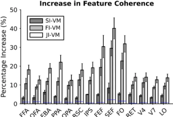
respects feature correlations, so they should better capture feature coherence. To test this prediction, we computed a voxelwise feature coherence metric and visualized it on flat maps (see Section 2.15). In Figure 5, feature coherence of voxelwise models is shown on the posterior part of the cortex of a representative subject (see Figures S7–S11 for all sub-jects). Feature coherence of FI-VM and JI-VM models is sig-nificantly higher than VM and SI-VM in all ROIs (p < .05, bootstrap test). In attention control areas, the increase in

feature coherence is very high (see Figure 6; 14.11 ± 1.59% for FI-VM and 20.45 ± 2.41% for JI-VM). In category-selec-tive areas, the increase in feature coherence is substantial (see Figure 6; 8.66 ± 1.35% for FI-VM and 14.33 ± 1.69% for JI-VM). In early visual areas, the increase is relatively mod-est (4.47 ± 0.67% for FI-VM and 6.65 ± 0.92% for JI-VM). These results suggest that informed feature regularization increases feature coherence particularly in attention control areas and high-level visual areas.

FIGURE 3 Cortical distribution of optimal L2-norm regularization parameter. The L2 regularization parameters over model features in the four VM methods (VM, FI-VM, SI-VM and JI-VM) are visualized on the right hemisphere of subject S1 (see Abbreviations). VM strictly penalizes model weights broadly across cortex. High regularization parameters reduce sensitivity in measuring voxelwise functional selectivity. Here, we incorporate additional regularization terms across features and across voxel neighborhoods. As such, the proposed method should limit unnecessary penalization of model weights by L2 regularization. As a result, compared to VM, FI-VM applies less weight regularization particularly in category-selective areas, early visual areas and frontal gyrus. Overall, JI-VM enforces the lowest weight penalization among the competing methods consistently across cortex. These results imply that both spatial and feature regularization alleviate the need for L2 regularization, thereby increasing sensitivity in measuring voxelwise functional selectivity [Colour figure can be viewed at wileyonlinelibrary.com]

FIGURE 4 Functional selectivity in a single voxel. Functional selectivity of two well-modeled voxels in EBA (extrastriate body area, voxel-1, S1) and PPA (parahippocampal place area, voxel-2, S2) is visualized for several object and action categories organized under the WordNet hierarchy. Each node represents the estimated response of the voxel to the labeled object (circles) or action category (squares). Red nodes correspond to categories that evoke above-mean responses, and blue nodes correspond to categories that evoke below-mean responses. Sizes of the nodes indicate the magnitude of the evoked responses. For visualization purposes, the model weights are normalized within each voxel. In the proposed approach, we incorporate feature and spatial regularization that limit unnecessary penalization of model weights by L2 regularization while improving prediction scores (R2 _{= .677 vs. R}2 _{= .839 for voxel-1 and R}2 _{= .029 vs. R}2 _{= .105 for voxel-2). Typically, a voxel in EBA is} expected to respond selectively to categories related to “human body” while a voxel in PPA is expected to respond selectively to categories related to “places.” Indeed, in voxel-1, functional selectivity for categories related to “body_parts” (e.g., “eye,” “hand,” “finger” and “arm”) is increased while the evoked BOLD activity by many unrelated categories is suppressed (subordinate categories of “vehicle,” “artifact,” etc.) in JI-VM compared to Classical VM. In voxel-2, functional selectivity for categories related to “scenes” (e.g., “road,” “landscape,” “street” and “path”) is increased. Furthermore, feature regularization enforces more similar weights in correlated categories. For example, in voxel-1, model weights of the subordinate categories of “structure” (e.g., “door,” “room” and “building”) or “motion” (e.g., “travel” and “walk”) are more similar in JI-VM compared to VM. Likewise, in voxel-2, model weights of the subordinate categories of “way” (e.g., “road,” “landscape,” “street” and “path”) are more similar in JI-VM compared to VM. Taken together, these results imply that feature and spatial regularization increase sensitivity in assessment of functional selectivity by enforcing functionally coherent model weights [Colour figure can be viewed at wileyonlinelibrary.com]

Spatial regularization enforces spatially coherent model weights for neighboring voxels, so SI-VM and JI-VM should yield higher spatial coherence compared to the alternative methods. To test this prediction, we computed a voxelwise spa-tial coherence metric and visualized it on flat maps (see Section 2.16). In Figure 7, spatial coherence of voxelwise models on the posterior part of the cortex of a representative subject is shown (see Figures S12–S16 for all subjects). SI-VM significantly in-creases and FI-VM significantly dein-creases spatial coherence

consistently in all ROIs (p < .05, bootstrap test). Meanwhile, JI-VM has significantly increased spatial coherence in all ROIs except RSC, FEF and FO (p < .05, bootstrap test). Yet, JI-VM shows significantly decreased spatial coherence in SEF. For JI-VM, the level of increase in coherence is higher in category-se-lective areas (10.19 ± 1.59%) than in attention control areas (2.38 ± 2.91%) and early visual areas (3.06 ± 0.85%; Figure 8). These results imply that spatial regularization yields improved spatial coherence broadly across cortex.

4

|

DISCUSSION

Voxelwise modeling (VM) is a powerful tool to model sin-gle-voxel selectivity for natural stimulus features with high sensitivity (Kay et  al.,  2008; Naselaris et  al.,  2009). Still, VM can yield suboptimal performance in the presence of high levels of measurement noise. Classical VM does not consider potential correlations among model features and spatial correlations among neighboring voxels. To improve performance, here we first introduced an informed feature regularization that considers feature correlations. We also introduced a spatial regularization approach that constructs voxel neighborhoods based on cortical distances. Our results indicate that the proposed approach provides more predictive voxelwise models for a natural vision experiment in many regions across cortex. We further measured the coherence of fit models, and our results suggest that improvements in pre-diction performance can be attributed to increased spatial and feature coherence across cortical representations.

Voxelwise modeling aims to estimate single-voxel func-tional selectivity from stimulus-driven fMRI data. Yet, VM may show suboptimal sensitivity in measuring selectivity in the presence of high noise levels and for complex stimu-lus models with thousands of features. Here, two sources of prior information were examined to alleviate this limitation, namely correlations among stimulus features and correlations among voxel responses. These priors were incorporated to

the VM framework as added feature and spatial regulariza-tion terms (both in JI-VM, feature reg. in FI-VM and spa-tial reg. in SI-VM). Note that regularized problem solutions require a careful trade-off between information from col-lected data (stimulus–response data) and prior knowledge. As FI-VM is constrained to only leverage feature regular-ization, it may alleviate noise at the expense of excessively increased feature coherence. Likewise, SI-VM can alleviate noise at the expense of over-increase in spatial coherence. (A similar problem is observed in traditional VM with excessive L2 regularization, Figure 3.) In contrast, JI-VM has increased

diversity in the type of prior information it can leverage. The success of a model in measuring functional selectivity should be primarily judged by the prediction scores. Thus, higher prediction scores of JI-VM compared to competing methods suggest that it can maintain a better balance between feature and spatial coherence while alleviating noise. However, it should also be noted that higher prediction performances of SI-VM and JI-VM over FI-VM come at the expense of in-creased computation time. Trade-off between high prediction performance and low computation time can be an important criterion in deciding which method to use.

With similar motivations to treat feature correlations, a recent study calculated a linear transformation of a category model to impose regularization with a non-uniform prior on model features (Nunez-Elizalde et al., 2018). The trans-formation was defined based on the dimensions of a word

FIGURE 5 Feature coherence for VM, FI-VM, SI-VM and JI-VM. Feature coherence for subject S1 is shown on the posterior part of the right hemisphere (see Abbreviations). VM ignores potential feature correlations in the stimulus, so it has reduced sensitivity to coherence in stimulus features. Informed feature regularization enforces similar model weights for correlated model features. Therefore, feature coherence of FI-VM and JI-VM is higher than that of VM and SI-VM across many cortical regions including category-selective areas, attention control areas and early visual areas. These results indicate that informed feature regularization better captures feature coherence broadly across visual cortex [Colour figure can be viewed at wileyonlinelibrary.com]

embedding space constructed using co-occurrence statistics in a large text corpus. It was reported that the proposed trans-formation approach yielded improved prediction scores for category models across significantly predicted cortical vox-els. As opposed to a transformation of model features, here we leave the model features in their original space and lever-age potential correlations through a graph Laplacian-based regularization term. Avoiding an additional transformation might offer an advantage in terms of interpretability of result-ing model weights. Our approach also allows for independent weighing of differences of model weights for each pair of cat-egory features. It remains important future work to compar-atively demonstrate the transformation versus regularization approach for treatment of feature correlations.

Regularization across model features has also been lev-eraged in neuroimaging studies beyond fMRI (Tran, Phung, Luo, & Venkatesh, 2015; Zhu, Suk, Wang, Lee, & Shen, 2015) or studies that focus on modeling natural stimuli (Sandler, Blitzer, Pratim Talukdar, & Ungar, 2008; Zhang & Ostendorf, 2012). A typical way that feature correlations are leveraged is to reduce dimensionality by eliminating redundant features from subsequent analyses. A previous study incorporated feature regularization to improve AD diagnosis performance with both regression and classifi-cation models (Zhu et  al.,  2015). The authors estimated similarity of neuroimaging features on MRI and PET im-ages, and then used these estimates to regularize correlated features during modeling. They have reported increased

FIGURE 6 Feature coherence across functional ROIs. Bar graphs display increases in feature coherence by the three methods (SI-VM, FI-VM and JI-FI-VM) over FI-VM (mean ± SD across subjects). Feature coherence of FI-VM and JI-VM models is significantly higher than that of VM in all functional ROIs (p < .05, bootstrap test). Threshold for significant improvement over Classical VM is designated with a blue line for each ROI. The average increase in attention control areas is 14.11 ± 1.59% for FI-VM and 20.45 ± 2.41% for JI-VM, whereas the average increase in category-selective areas is 8.66 ± 1.35% for FI-VM and 14.33 ± 1.69% for JI-VM and the average increase in early visual areas is 4.47 ± 0.67% for FI-VM and 6.65 ± 0.92% for JI-VM. In contrast, SI-VM that lacks feature regularization has relatively limited increase in feature coherence across all ROIs. These results suggest that informed feature regularization increases functional coherence in cortical representations particularly in areas that take part in attention control and high-level visual functions [Colour figure can be viewed at wileyonlinelibrary.com]

FIGURE 7 Spatial coherence for VM, FI-VM, SI-VM and JI-VM. Spatial coherence for subject S1 is shown on the posterior part of the right hemisphere (see Abbreviations). VM ignores correlations among voxel neighborhoods, so it has reduced sensitivity to spatial coherence in cortical representations. Spatial regularization enforces increased spatial coherence among cortical representations within voxel neighborhoods. Although FI-VM and VM have relatively similar spatial coherence values, SI-VM and JI-VM yield higher spatial coherence consistently across many cortical regions. These results suggest that spatial regularization better captures spatial coherence broadly across visual cortex [Colour figure can be viewed at wileyonlinelibrary.com]

regression and classification performance in AD diagnosis. In another study on medical risk stratification, the authors implemented feature regularization on various features ex-tracted from electronic medical records (EMRs) on differ-ent timescales during ordinal regression (Tran et al., 2015). They have reported that suicide risk can be better predicted by a model of EMR-derived features compared to clini-cians. In both studies, the authors discarded redundant features via an L1-norm regularization. Unlike these pre-vious studies, here we retained all stimulus features in the model. Several previous studies have employed a feature regularization approach similar to the one proposed here for robust text classification (Sandler et al., 2008; Zhang & Ostendorf, 2012). In Zhang et al., the authors regularized the correlated subtopics for a discriminative classifier. They constructed a feature affinity matrix using subtopic co-oc-currences on a large unlabeled dataset as in our method. Later, they included a feature regularization term based on the feature affinity matrix into maximum entropy training objective. They have reported that feature regularization on subtopic features improved text classification accuracy

over other semi-supervised learning approaches. In Sandler et al., the authors incorporated feature regularization into sentiment classification and newsgroups document classi-fication via logistic regression. Similar to our approach, they used a graph Laplacian-based regularization by using both word co-occurrences and prior domain information to compute feature similarities. They have reported improved classification performances over many other semi-super-vised learning methods.

The proposed method leverages a linguistic model to guide feature regularization on a visual category model. Indeed, several recent studies suggest that category infor-mation in natural visual scenes is well captured by semantic features in natural language. Clarke et al. reported that visual objects that shared a superordinate category yielded more similar activation patterns in perirhinal cortex than those that did not (Clarke & Tyler, 2015). Carlson et al. reported that se-mantically related objects had similar neural representations in inferior temporal cortex (Carlson, Simmons, Kriegeskorte, & Slevc, 2014). Semantic relatedness was measured using hi-erarchical word relations and distributional patterns of words in large text corpora. More recently, Wen et al. reported a significant correlation between representational similarity and semantic similarity across cortex for a pair of visual ob-jects (Wen, Shi, Chen, & Liu, 2018). In that study, seman-tic similarity was measured based on the distances in word embedding models (Landauer, 2006; Pennington, Socher, & Manning, 2014).

Here, we used a common set of hyperparameters for con-structing the feature Laplacian matrix and spatial Laplacian matrix. A potential avenue for improvement for the proposed method is to consider voxelwise optimization of these pa-rameters. Note, however, that this will require considerably higher computational load. Improving performance in feature regularization might also be viable via different approaches to computing similarity of model features. Here, we calcu-lated them in the word embedding space constructed using co-occurrence statistics. One can typically utilize another word embedding space constructed by word2vec or LSA to find the similarities of model features (Landauer, 2006; Mikolov, Yih, & Zweig, 2013).

In summary, we introduced a novel voxelwise modeling approach that simultaneously utilizes stimulus correlations in model features and response correlations among voxel neigh-borhoods. Our results indicate clear improvements in predic-tion performance, spatial coherence and feature coherence of category models in a natural vision experiment, specifically across visual category areas and attention control areas. With little increase in computation time, a significant albeit mod-est improvement in prediction performance is obtained with feature regularization compared to spatial regularization. Meanwhile, concurrent use of spatial and feature regulariza-tion yields even higher predicregulariza-tion performance with further

FIGURE 8 Spatial coherence across functional ROIs. Bar graphs display increases in spatial coherence by the three methods (FI-VM, SI-VM and JI-SI-VM) over SI-VM (mean ± SD across subjects, see Abbreviations). Spatial regularization enforces increased spatial coherence among cortical representations of neighboring voxels. Threshold for significant improvement over Classical VM is designated with a blue line for each ROI. SI-VM has significantly higher spatial coherence than VM in all functional ROIs (p < .05, bootstrap test). JI-VM has significantly higher spatial coherence than VM in all functional ROIs except RSC, FEF, SEF and FO (p < .05, bootstrap test). The average increase in category-selective areas is 17.00 ± 0.69% for SI-VM and 10.19 ± 1.59% for JI-VM, whereas the average increase in attention control areas is 14.89 ± 1.29% for SI-VM and 2.38 ± 2.91% for JI-VM and the average increase in early visual areas is 7.89 ± 0.22% for SI-VM and 3.06 ± 0.85% for JI-VM. Meanwhile, FI-VM that lacks spatial regularization does not yield any improvement in spatial coherence. These results indicate that spatial regularization increases spatial coherence among cortical representations of voxel neighborhoods across many cortical regions [Colour figure can be viewed at wileyonlinelibrary.com]