Censored Nonparametric Time‑Series Analysis
with Autoregressive Error Models
Dursun Aydin1 · Ersin Yilmaz1 Accepted: 18 June 2020
© Springer Science+Business Media, LLC, part of Springer Nature 2020
Abstract
This paper focuses on nonparametric regression modeling of time-series observa-tions with data irregularities, such as censoring due to a cutoff value. In general, researchers do not prefer to put up with censored cases in time-series analyses because their results are generally biased. In this paper, we present an imputation algorithm for handling auto-correlated censored data based on a class of autore-gressive nonparametric time-series model. The algorithm provides an estimation of the parameters by imputing the censored values with the values from a truncated normal distribution, and it enables unobservable values of the response variable. In this sense, the censored time-series observations are analyzed by nonparametric smoothing techniques instead of the usual parametric methods to reduce model-ling bias. Typically, the smoothing methods are updated for estimating the censored time-series observations. We use Monte Carlo simulations based on right-censored data to compare the performances and accuracy of the estimates from the smooth-ing methods. Finally, the smoothsmooth-ing methods are illustrated ussmooth-ing a meteorological time- series and unemployment datasets, where the observations are subject to the detection limit of the recording tool.
Keywords Censored time series · Penalized spline · Smoothing spline · Auto-correlated data · Imputation method
* Ersin Yilmaz [email protected]
Dursun Aydin [email protected]
1 Department of Statistics, Faculty of Science, Mugla Sitki Kocman University, 48000 Mugla, Turkey
1 Introduction
In the statistical literature, researchers use the term “right-censored observation” for a unit’s failure time that is only known to exceed a detection limit. Gener-ally, the measurements collected over time are observed with data irregularities, such as censoring due to a threshold value. Ordinary statistical methods cannot be applied directly to such observations, especially for time-series data. As is known, time-series measurements are often auto correlated and analyzed by mod-eling autocorrelations via their appropriate autoregressive structures. Box and Jenkins (1970) presented the first study dealing with time-series analysis within a parametric framework. However, although parametric approaches are highly use-ful for analyzing time-series data, they can produce biased estimates or lead to wrong conclusions, especially for censored data.
When using time series, we may encounter severe problems using data with censored or auto-correlated errors. During the last decade, many techniques have been proposed for dealing with such problems in which the dependent variable is subject to censoring. Our view is that these techniques are fundamentally divided into parametric and nonparametric methods, depending on the estimated autocor-relation function. Here, we focus only on the nonparametric approaches and try to discern which will provide a better estimation of auto-correlated censored data.
Suppose we consider a nonparametric time-series regression model with autoregressive errors for censored response observations at time t, given by where Yt represents a stationary time series, and its prediction depends on the
explanatory variable Xt , and f is an unknown smooth function giving the conditional
mean of Yt given Xt . In addition, et , defined in (1), is a stationary autoregressive
error term generated by where 𝜙 = (𝜙1,… , 𝜙p
)⊤
is the vector of the autoregressive coefficients and 𝜀t
repre-sents independent and identically distributed random variables with zero mean and variance 𝜎2 . Model (1) does not contain lagged Y′
ts and has auto-correlated error
terms. This makes it an appropriate model for the regression analysis of certain kinds of time-series data.
Our objective is to estimate both the unknown function f (.) and the autore-gressive structure in (1) by nonparametric methods using censored time- series data. There are numerous studies suitable for the estimation approaches of f (.) in a nonparametric regression model based on censored data (Zheng 1984; Dab-rowska 1992; Kim and Truong 1998; Yang 1999; Cai and Betensky 2003; and Aydin and Yilmaz 2017). As noted, while there are extensive studies on estimat-ing nonparametric models with censored responses, the literature on censored time-series response data is limited. Examples of these works include Zeger and Brookmeyer (1986), Park et al. (2007), and Wang and Chan (2017).
(1)
Yt= f(Xt)+ et, t= 1, … , n
(2)
Problems with censored time- series data are commonly solved using data aug-mentation techniques. Several researchers, including Robinson (1983), Parzen (1983), Tanner (1991), Hopke et al. (2001), and Park et al. (2007, (2009), have used this technique for regression models with autoregressive errors when cen-sored response observations are considered. Note that both imputation and aug-mentation methods are addressed by several authors for missing values, excluding time- series observations. For example, see the studies of Rubin (1996), Dempster et al. (1977), Heitjan and Rubin (1990), and Meng (1994). In addition, there are several nonparametric estimation methods for obtaining the autocovariance func-tion in the literature, such as Hall and Patil (1994), who suggested a nonparamet-ric estimation method for estimating the autocovariance function based on kernel smoothing (KS). Elogne et al. (2008) estimated the autocovariance function with interpolation techniques, and there are several similar studies: Glasbey (1988), Shapiro and Botha (1991), Sampson and Guttorp (1992), Bjørnstad and Grenfell (2001), and Wu and Pourahmadi (2003).
In the literature, there are essentially two approaches to handling censoring. One is to eliminate the censored values, and the other is to use the censored data points as observed. However, the study of Park et al. (2007) demonstrates that both approaches yield biased and inefficient estimates. It is possible that the per-formance of the parameter estimation can be improved by using datasets that have a lower censoring rate (Helsel 1990). However, such methods are often not appli-cable, and outcomes depend heavily on rigid parametric model assumptions. As indicated above, even though some numerical solutions have been proposed in the literature to cope with the problem of censored responses in autoregressive error models, there are no studies making inferences for censored time-series models in terms of nonparametric approaches. By contrast, we propose nonparametric estimation procedures for time-series containing right-censored observations, instead of using parametric approaches. Thus, our study is remarkably different from other similar studies used in the statistical literature.
In this paper, we consider three nonparametric approaches, smoothing spline (SS), kernel smoothing (KS), and regression (penalized) spline (RS), for estimat-ing an autoregressive time-series regression model with right- censored obser-vations. Note that these nonparametric approaches cannot be applied directly to censored observations, and a data transformation is required to estimate the cen-sored response observations. To overcome this problem and to get stable solu-tions, we used a data augmentation method, namely a the Gaussian imputation technique. This data transformation method, which is a modified extension of ordinary Gaussian imputation, is used to adjust the censoring response variable in the setting of a time series. We also compare the performances of the smoothing methods with the benchmark AR(1) model. To the best of our knowledge, such a study has not been conducted. It should be noted that the best estimation of the censored lifetime observations Yt that depend on an explanatory variable Xt= x
could be expressed as the conditional mean of the response E(Yt|Xt= x) = f (x) ,
Normally, it is not necessary that function f be linear, and the conditional variance is homoscedastic, but the error term indicated in model (1) is generally presented as follows
As indicated above, the minimization of Eq. (3) is carried out through three smooth-ing methods, the SS, KS , and RS methods. The primary purpose of this study is to estimate a right-censored time series non- parametrically and provide consistency in the estimation with the help of the data augmentation method for censored observa-tions. One of the important points of data augmentation is to estimate the covariance function (Park et al. 2009). Here, this function is estimated with a nonparametric Nadaraya-Watson estimator. With this method, there is no need to describe the prior distribution of the time- series data because data augmentation is achieved using the nonparametric method.
The paper is organized as follows. Section 2 introduces the thory of the censored autoregressive model and algorithm of Gaussian imputation to make data augmenta-tion. In Sect. 3, the three smoothing methods are explained, and their modifications are illustrated according to censored data. Section 4 involves the evaluation measurements for the three modified smoothing techniques. Furthermore, an estimation of the covari-ance functions of the estimators are expressed. To obtain empirical results, a detailed simulation study is done in Sect. 5. Also, two real-data applications with cloud and unemployement datasets are realized in Sect. 6. Finally, conclusions and discussion are presented in Sect. 7.
2 Censored Autoregressive Model and Preliminaries
Consider the nonparametric regression model defined in Eq. (1). In many applications, we may be unable to directly observe the response variable Yt . Instead of attempting to
observe all the values of the response variable, we may observe only Yt when Yt exceeds
a constant value Ct that denotes a cut-off value or a detection limit. Time- series
obser-vations are often obtained with a detection limit. For example, a monitoring tool usu-ally has a detection limit, and it records the limit value when the true value exceeds the detection limit. This case is often called censoring, which is also a type of missing data mechanism. Censoring of the response measurements occurs in different situations in the physical sciences, business, and economics. If censored observations are ignored, the resulting parameter estimates are usually biased.
Let Zt be the value we observe instead of Yt due to censoring. Then, in the
right-censored cases, we consider the following type of censoring, given by
(3) E{Yt− f (x)}2= E { Yt− ̂Yt }2 E(𝜀t|Xt)= 0 , Var(𝜀t|Xt)= 1. (4) Zt= min(Yt, Ct),𝛿t= I(Yt≤ Ct)
where I(.) is an indicator function,𝛿 = 0 denotes a censored observation, and
Zt and Ct are the failure times (or observed lifetimes) and the censoring times,
respectively. In light of (4), we assume that only the response variable Yt is
cen-sored on the right by censoring variable Ct , so our observations are the triples
{
(Zt, 𝛿t, Xt), t = 1, 2, … , n
}
. Then, model (1) along with Eq. (4), reduce the
cen-sored autoregressive nonparametric regression model of order p. It should be noted
that Yt and Zt have different distributions. Therefore, Zt cannot be used directly to
make inferences about model (1) described by Yt . To use the Zt series as a response
variable, a conditional distribution is constructed through a truncated normal distribution.
Assume that Yt= (Y1,… , Yn)
⊤ is a realization from a stationary time series
described by model (1) with autoregressive error terms, which has a Gaussian disturbance 𝜀t , as defined in (2). Note that the autoregressive errors follow an n-dimensional multivariate normal distribution with a mean zero and stationary n× n covariance matrix Σ. In other words, et= (e1,… , en)⊤∽ Nn(0, 𝚺) , where 𝚺= 𝜎2R
n(𝜙) is a n × n covariance matrix, given by
where 𝛾0,𝛾1,… , 𝛾n−1 are theoretical autocovariances of the process and
𝜌h={𝛾h∕𝛾0, h= 1, 2, .., p
}
are the theoretical autocorrelations of the process. It should be noted that 𝛾h= E(𝜀t𝜀⊤t−h) denotes the autocovariance at lag h and
𝛾0 = E(𝜀t𝜀⊤
t
)
= 𝜎2 gives the constant variance at lag zero.
In light of the equations and explanations outlined above, it is understood that
Yt∼ Nn(𝝁, 𝚺) for complete data. When we consider the responses with a
cen-soring mechanism, as in (4), Yt∼ TNn(𝝁, 𝚺;Rc) , where TNn(. ; Rc) denotes the
truncated normal distribution on the interval Rc (see Vaida and Liu (2009) for a
more detailed discussions). Note that the interval Rc depends on whether a data
point is censored. Basically, the interval Rc is
(
0, Ct) if 𝛿t= 1(observed values) and
Rc is [Ct,∞) if 𝛿t= 0 (censored values) . To calculate the unknown function in the
censored autoregressive nonparametric regression model, the first task is to con-sider separately the observed and censored data points of the response variable at the beginning of the estimation procedure. In this context, by using permutation matrix P, which maps (1, … , k)⊤ into the permutation vector p = (p
1,… , pk)⊤ , the
order of the data can be rearranged as
where Yo denotes the observed part of the Yt′s , whereas Yc indicates the right-
cen-sored part of the same variable. Furthermore, PYt provides a multivariate normal
distribution defined by Rn(𝜙) = 1 𝜎2 𝜀t ⎛ ⎜ ⎜ ⎜ ⎝ 𝛾0 𝛾1 … 𝛾1 𝛾0 … ⋮ 𝛾n−1 ⋮ 𝛾n−2 ⋱ … 𝛾n−1 𝛾n−2 ⋮ 𝛾0 ⎞ ⎟ ⎟ ⎟ ⎠ = ⎛ ⎜ ⎜ ⎜ ⎝ 1 𝜌1 … 𝜌1 1 … ⋮ 𝜌n−1 ⋮ 𝜌n−2 ⋱ … 𝜌n−1 𝜌n−2 ⋮ 1 ⎞ ⎟ ⎟ ⎟ ⎠ (5) PYt= ( Po Pc ) Yt= ( Yo Yc )
where 𝚺oo= E
[
(Yo− 𝝁o)(Yo− 𝝁o)⊤] shows the covariance matrix obtained by
taking the observed part of the Yt , while 𝚺cc= E
[
(Yc− 𝝁c)(Yc− 𝝁c)⊤] states the
covariance matrix that corresponds to the right-censored data points of the Y′
ts , and 𝚺oc= 𝚺co=[(Yc− 𝝁c)(Yo− 𝝁o)⊤].
It should be noted that the conditional distribution of Yc given Yo is also a
multivari-ate normal distribution with parameters 𝝁 and 𝚺 (see, for example, Anderson 1984). In a similar manner to that used to obtain (5), the observed data vector Zt can be portioned
into sub-vectors, and is given by
One of the reasons for the study of conditional distribution derived from the multi-variate normal distribution outlined above is to find an appropriate substitute for the right-censored data vector Zc . The basic idea is to replace the elements of the
right-censored vector Zc by sampling values obtained from the conditional distribution
of the censored response vector Yc given Zo and Zc . This procedure is equivalent to
applying the truncated multivariate normal distribution (Park et al. 2007):
wherenc denotes the number of censored data points, TNncshows a truncated
multi-variate normal distribution with nc-dimension, and Rc determines the region
asso-ciated with the censoring of the response observations, as previously defined. The symbols M and V expressed in (8) are the parameters that correspond to the condi-tional mean and covariance of a non-truncated variant of a condicondi-tional multivariate normal distribution.
Now, suppose that we have a time-series vector Yt= (Y1,… , Yn)⊤ that can be
parametrized by the mean 𝜇 , variance 𝜎2 , and autocorrelation 𝜌 . As indicated
above, these time series measurements are also considered a random vector from a multivariate normal distribution Yt ∼ Nn(𝝁, 𝚺) where 𝝁 = 𝜇1n and
{𝚺}i,j= E ( ete⊤ t ) = 𝜎2 et= 𝜎2 𝜀t
1−𝜌2𝜌|i−j|, i, j= 1, … , n . The conditional distribution of Zt ,
given other observations, is a univariate normal distribution; if Zt is censored, then
the conditional distribution is a truncated univariate normal distribution. Many sta-tistical approaches for obtaining the truncated normal distribution depend on a compacted simulation. Examples of such studies include Tanner and Wong (1987), Chen and Deely (1996), Gelfand et al. (1992), and so on. In general, the mentioned studies focus on the data augmentation method with a truncated normal distribu-tion, Bayesian methods, and Gibbs samplers. In this study, we use a truncated nor-mal distribution whose probability density function can be defined as
(6) PYt∼ Nn ( 𝝁 ( Po Pc ) , [ Po𝚺P⊤o Po𝚺P⊤c Pc𝚺P⊤o Pc𝚺P⊤c ]) = Nn (( 𝝁o 𝝁c ) , [ 𝚺oo 𝚺oc 𝚺co 𝚺cc ]) (7) PZt= ( Po Pc ) Zt= ( Zo Zc ) (8) ( Yc|Zo,Zc∈ Rc ) ∼ TNnc ( M,V, Rc ) (9) f(Zt)= g(Zt)I(𝛿t= 0)∕ [ 1− F(Ct)]
where I(.) denotes the indicator function, that is, I = 1 if 𝛿t= 0 , and g(.) and F(.) are
the probability density function of the standard normal distribution and its cumula-tive distribution function, respeccumula-tively. It should be noted that Gaussian density g(.) is used for observations in the interval [Ct,∞] to obtain the distribution of the
right-censored part of the data.
In this paper, we focus on the data imputation method to find a solution to the sored data problem. One should note that the basic idea in the imputation of the cen-sored values is to replace every cencen-sored observation with a real value. To carry out this procedure, in the first stage, the parameters of the distributions outlined above must be estimated by iteratively applying an appropriate algorithm.
2.1 Imputation Algorithm
Let 𝛗 = (𝝁, 𝚺) be the true parameter vector based on the distribution of Yt with
auto-correlation 𝜌 and 𝚽 = (M, V) be a parameter vector based on the conditional distri-bution of the censored response variable Yc . By introducing the censored variable to
the model (1), the imputation algorithm simplified to the generation of values from the truncated normal distribution defined in (9). Usually, all the censored observations are set equal to some constant value. The idea of the algorithm is to update the parameter estimates by filling (or imputing) the censored values with the values from a condi-tional sample. The iteratively updated algorithm is essentially divided into two compo-nents: data augmentation and parameter estimation. It should be emphasized that one needs to use a random sample generated from a truncated multivariate normal distribu-tion for data augmentadistribu-tion, whereas any tradidistribu-tional method for the parameter estima-tion can be used.
The imputation algorithm consists of the following steps:
Step 1 Generate the truncated normal distribution and compute the density of the
censored partition of the data.
Step 2 Obtain the initial parameter estimates ̂𝜇(0) , ̂𝜌(0) , and ̂𝜎(0) by using the
equations ̂ 𝜌(0) = � ∑n t=2 � Zt−1(0)− Z−n(0)� 2�−1�∑ n t=2 � Zt(0)− Z (0) −1 �� Zt(0)−1− Z (0) −n �� , and
where notation ̂𝜇(0) denotes the estimated mean for iteration zero,
Z(0) −n = (n − 1) −1∑n−1 t=1Zt and similarly Z (0) −1 = (n − 1) −1∑n t=2Zt . By using Step 1,
determine the initial estimates of parameter vector (𝝁, 𝚺) :
̂ 𝜇(0)= n−1 n ∑ i=1 Zt(0), ( ̂ 𝜎(0)) 2 = (n − 3)−1 n ∑ t=2 ( Zt(0)− ̂𝜇(0)− ̂𝜌(0)(Zt(0)−1− ̂𝜇(0))) 2
Step 3 Compute the conditional mean and variance ̂M(0)and ̂V
(0)
based on the cen-sored part of the parameter vector 𝚽 = (M, V) according to
̂ M(0) = ̂𝜇(0)c + ̂Σ(0)co(Σ̂(0)oo) −1( Zo− ̂𝜇 (0) o ) and,
where covariance matrices are described in (6).
Step 4 Generate the vector Z(1)
c of the right-censored observations from truncated
normal distribution, TNnc
(
̂
M(0), ̂V(0), Rc )
, where Rc denotes the interval [Ct,∞).
Step 5 By applying the instructions expressed in Eqs. (5) and (7), construct the
following augmented data from the observed part and the vector Z(1)
c defined in the
previous step:
Step 6 Re-compute the estimates of the parameter 𝜇 , 𝜎2 , and 𝜌 according to Z(1) and
update the parameters 𝚺 , M, and V , as defined in Steps 2 and 3.
Step 7 Repeat the algorithm from Step 2 to Step 6 under the condition 𝜓 < 0.005
(for our simulations). Note that 𝜓 indicates the convergence ratio of the parameter estimates at the kth iteration, given by
where 𝜽 = ( 𝜇, 𝜎2,𝜌 )⊤ denotes the parameter vector.
We should recall, as stated about the imputation algorithm, we are not restricted to a specific method for the parameter estimation. For the autoregressive time- series models, once the augmented data is obtained, any suitable method (for example, Yule–Walker, least squares, or maximum likelihood) can be used to estimate the parameters (see, Park et al. 2007). In this paper, we update the
smoothing splines(SS), kernel smoothing (KS), and regression spline (RS) methods
to estimate the parameters of the nonparametric autoregressive time- series model with right-censored data.
3 Modified Estimation Methods
In this section, we introduce three different modified estimation procedures to estimate the unknown function in the autoregressive time- series model, which is defined in (1). The modified methods are based on a generalization of the ordinary
̂ 𝝁(0)= ̂𝜇(0)1n, {𝚺 }i,j= {( ̂ 𝜎(0))2 /( 1−[𝜌̂(0)]2 )} ̂ 𝜌(0)|i−j|, i, j= 1, … , n, ̂ V(0)= ̂Σ(0)cc − ̂Σ(0)co(Σ̂(0)oo) −1 ̂ Σ(0)oc Z(1)= P−1 [ Zo Z(1)c ] . (10) 𝜓 =[(�𝜽(k+1)− �𝜽(k) )⊤( � 𝜽(k+1)− �𝜽(k) )]/( � 𝜽(k) )⊤ � 𝜽(k)
SS, KS, and RS methods or conventional censored nonparametric regression
mod-els. Examples studies using mentioned methods include Zheng (1998), Dabrowska (1992), Fan and Gijbels (1994), Guessoum and Ould Said (2008), Aydin and Yilmaz (2017).
3.1 Smoothing Splines
Now we consider ways to estimate the unknown regression function f(x) stated in model (1), where E(Yt|Xt= x
)
= f (x) . The first way to approach to the nonparamet-ric regression is to fit a spline with knots at every data point. The main idea is to find a regression function f (.) that minimizes the penalized residual sum of squares (PRSS) criterion
where Z(k)
t is the response variable that provides the criterion (10) at the kth iteration, f ∈ C2[a, b] is a unknown smooth function, and 𝜆 is a positive smoothing parameter,
controlling the tradeoff between the closeness of the estimate to the data and rough-ness of the function estimate. If 𝜆 → ∞ , the roughrough-ness penalty term dominates and the the parameter 𝜆 forces f��
(x) → 0 , yielding the linear least squares estimate. If
𝜆 → 0 , the penalty term becomes negligible, and the solution tends to an
interpo-lating estimate. Therefore, the choice of the smoothing parameter is an important problem and the GCV method has been used to address this problem in this paper. Note that minimizing the PRSS in (11) over the space of all continuous differenti-able functions leads to a unique solution, and this solution is a natural cubic spline with knots at the unique values x1,… , xn for a fixed smoothing parameter 𝜆.
Suppose that f is a natural cubic spline (NCS) with knot points x1< ⋯ < xn . By
giving its value and second derivative at each knot points we can determine the fol-lowing NCS vectors
and
that specify the curve f completely. However, not all possible vectors f and 𝝑 repre-sent NCSs. In this sense the following theorem, discussed by Green and Silverman (1994), provides a condition for the vectors to be an NCS on the given knot points.
Theorem 3.1 (Green and Silverman 1994). The vectors f and 𝝑 determine an NCS f
if and only if the following criterion
(11) PRSS(f , 𝜆) = n ∑ t=1 { Zt(k)− f(Xt )}2 + 𝜆 � b a { f��(x)}2dx, a≤ x1≤ ⋯ ≤ xn≤ b f(Xt)=(f(x1),… , f (xn) )⊤ = (f1,… , fn) ⊤ = f f��(Xt ) =(f��(x2 ) ,… , f��(xn−1 ))⊤ =(𝜗2,… , 𝜗n−1 )⊤ = 𝝑 (12) Q⊤f= R𝝑
is satisfied. If Eq. (12) is satisfied, then the roughness penalty term will provide
A useful algebraic result from Theorem 3.1 is that the penalty term in (11) may be
written in quadratic form. In matrix and vector form, the criterion in (11) can be
rewritten as
Notice that Kin Eqs. (13) and (14) is a symmetric n × n positive definite penalty
matrix that can be decomposed to
where Q is a tri-diagonal (n − 2) × n matrix with elements Qii= 1∕hi ,
Qi,(i+1)=(1
hi +
1
hi+1
)
, and Qi,(i+2)= 1∕hi+1 , R is a symmetric tri-diagonal matrix of
order (n − 2) with R(i−1),i= Ri,(i−1) = hi∕6 , Rii=
(
hi+ hi+1
)
∕3 , and hi= xi+1− xi
denotes the distance between successive knot points.
For some constant 𝜆 > 0 , the corresponding solution based on the smoothing splines (SS)for the vector f , which specify the unknown smooth function f in (1), can be obtained by
where 𝚺 is the n-dimensional regularity matrix for autocorrelated errors and
SSS𝜆 = (𝚺 + 𝜆K)−1𝚺 is a positive definite spline smoother matrix that depends on
parameter 𝜆 . Details on the derivation of Eq. (15) can be found in the “Appendix 1”.
3.2 Kernel Smoothing
As explained in the imputation algorithm, the idea is that, instead of Yt , we consider the
response variable Z(k)
t , which is employed to estimate the censored observations. In this
case, model (1) reduces to the following nonparametric regression model
This model can be considered as equivalent to the regression model with autore-gressive errors. Consequently, kernel smoothing can be used as an alternative non-parametric approach to (SS) to get a suitable estimate of function f. Analogous to (15), this leads to the kernel regression estimator, in other words, (KS) introduced by Nadaraya (1964) and Watson (1964). Accordingly, the estimate of f (.) at fixed x can be computed by (13) ∫ b a { f��(x)}2dx= 𝝑⊤R𝝑= f⊤Kf (14) PRSS(f, 𝜆) = ‖‖‖Z(k)− f‖‖‖2 2+ 𝜆f ⊤Kf. K= Q⊤R−1Q (15) ̂f𝜆SS= (𝚺 + 𝜆K)−1𝚺Z(k)= SSS𝜆Z(k) (16) Z(k)t = f(Xt)+ et, t= 1, … , n
where SKS
𝜆 is a kernel smoother matrix defined by weights
with a bandwidth 𝜆 (also called a smoothing parameter), which is a nonnegative number determining the degree smoothness of ̂f𝜆KS(x) , as in (SS). In fact, it is
pos-sible to write the weighted sum (17) in a more general form
In the expressions above, K(u) is a real-valued kernel function assigning weights to each data point, and the kernel K satisfies the following conditions: (u) ≥ 0 , ∫ K(u)du = 1 , and K(u) = K(−u) for all u ∈ R . Moreover, Eq. (19) shows that the kernel regression estimator is a weighted average of the response observations Z(k)
t .
Also, as expressed above, the 𝜆 is a critical parameter in kernel regression esti-mation. A large bandwidth 𝜆 provides an over-smooth estimate, whereas a small bandwidth 𝜆 produces a wiggly function curve. For example, when 𝜆 → 0 , then
w𝜆(x, Xt
)
→ n , and hence, the estimator (17) reproduces the response observations (i.e., ̂fKS 𝜆 (x) → Z (k) t ). When 𝜆 → ∞ , then s𝜆 ( x, Xt )
→ 1 , and the estimator (17) con-vergences to the mean of the response observations (i.e., ̂fKS
𝜆 (x) → Z
(k)
t ). In this
con-text, the GCV method is used in to determine the amount of smoothness required, as with the SS method.
3.3 Regression Spline
One alternative approach to estimating a function non-parametrically is to fit a qth-order RS (or penalized spline), which can be computed in terms of truncated power functions. To be specific, it is assumed that the unknown univariate function f (.) can be estimated by a penalized spline with a truncated polynomial basis
where 𝜆 is a positive smoothing parameter, as in the other two approaches, q is the degree of spline, {𝜅r, r= 1, … , m} are spline knot points,
(17) ̂f𝜆KS(x) = n ∑ t=1 Σtw𝜆 ( x, Xt)Z(k)t = SKS𝜆 Z(k) (18) s𝜆 ( x, Xt ) = K (X t− x 𝜆 ) ∕ n ∑ t=1 K (X t− x 𝜆 ) = K(u)∕∑K(u) (19) ̂f KS 𝜆 (x) = n−1∑nt=1K(u)Zt(k) n−1∑n t=1K(u) = 1 n n � t=1 ⎛ ⎜ ⎜ ⎜ ⎝ K �X t−x 𝜆 � n−1∑n t=1K �X t−x 𝜆 � ⎞ ⎟ ⎟ ⎟ ⎠ Zt(k)= 1 n n � t=1 Σts𝜆�x, Xt�Z(k)t (20) f(Xt)= b0+ b1Xt+ b2X 2 t + ⋯ + bqX q t + 𝜆 m ∑ r=1 bq+r(Xt− 𝜅r )q +
is a set of regression coefficients, (Xt− 𝜅r )q += ( Xt− 𝜅r )q
when Xt> 𝜅r and
oth-erwise (Xt− 𝜅r
)q
+= 0 . It is also assumed that min
(
Xt) < 𝜅1< ⋯ < 𝜅m<max(Xt) ,
such that spline knot points {𝜅1,… , 𝜅m
}
represent a subset of {X1,… , Xn
} (see, Ruppert 2002 for knot selection).
It follows from Eq. (20) that, for a truncated polynomial basis, the nonparametric time-series model (1) is
where Z(k)
t is the observed response variable, as with the previous two approaches.
As displayed in the Eq. (21), the truncated qth-degree power basis with knots 𝜅r has
basis vectors. In a matrix and vector form, model (21) can be rewritten as where Z(k)= ⎡ ⎢ ⎢ ⎣ Z1(k) ⋮ Z(k) n ⎤ ⎥ ⎥ ⎦ , = ⎡ ⎢ ⎢ ⎣ 1 X1 … X q 1 � X1− 𝜅1 �q + … � X1− 𝜅m �q + ⋮ 1 Xn … Xnq � Xn− 𝜅1 �q + … � Xn− 𝜅m �q + ⎤ ⎥ ⎥ ⎦ , b = ⎡ ⎢ ⎢ ⎢ ⎣ b0 b1 ⋮ bq+m ⎤ ⎥ ⎥ ⎥ ⎦ , and e= ⎡ ⎢ ⎢ ⎣ e1 ⋮ en ⎤ ⎥ ⎥ ⎦ .
For the penalized- spline- fitting problem, the key is to choose the vector b that minimizes
where D = diag(0(q+1), 1m) is a diagonal penalty matrix whose first (q+1) elements are 0 and whose other elements are 1. Note that 𝜆 ∑m
r=1b 2
q+r= 𝜆b
⊤Db in (23) is
referred to as a penalty term whose magnitude is determined by a positive smooth-ing parameter 𝜆 . It is clear that 𝜆 plays an important role in estimatsmooth-ing the regression model. As with the (SS) and the (KS) expressed in the previous sections, 𝜆 is selected by a GCV criterion.
Minimization of the Eq. (23) yields to estimates of the vector b, where For (24) the fitted values ̂f based on the (RS) can be stated as
{ b0, b1,… , bq, bq+1,… , bq+m } (21) Zt(k)= b0+ b1Xt+ b2Xt2+ ⋯ + bqX q t + 𝜆 m ∑ r=1 bq+r(Xt− 𝜅r)q+ + et, t= 1, … , n (22) Z(k)= Xb + e (23) PRSS(b, 𝜆) = n ∑ t=1 Σt(Zt(k)− f(Xt)) 2 + 𝜆 m ∑ r=1 b2q+r= 𝚺‖‖‖Z(k)− Xb‖‖‖2 2+ 𝜆b ⊤ Db (24) � b=(X⊤𝚺X+ 𝜆D)−1X⊤𝚺Z(k) (25) �f𝜆RS= X�b= X(X⊤𝚺X+ 𝜆D)−1X⊤𝚺Z(k)= SRS𝜆 Z(k)
where SRS
𝜆 = X
(
X⊤𝚺X+ 𝜆D)−1X⊤𝚺 is the smoother matrix based on the penalized
spline that is dependent on a smoothing parameter 𝜆 , as in the other smoother matri-ces. Details on the derivation of Eq. (25) can be found in “Appendix 2”.
The penalized spline method uses polynomial functions to best fit the data and includes a penalty term to prevent the overfitting problem. Thus, the method can produce more accurate estimates. As noted, the penalized spline fits the model with the help of specified nodes. These nodes need to be optimally selected. In this paper, the full search algorithm is used for selecting the nodes defined by Ruppert et al. (2003). For more details about knot selection using censored data, see the study of Aydin and Yilmaz (2017).
4 Evaluating the Performance of the Estimators
For a given smoothing parameter 𝜆 the regression estimators studied here (such as smoothing spline, kernel and regression spline) can be written in the form
where Z(k)
= ( Z1(k),… , Z(k)
n )
� and S
𝜆 is a n × n dimensional smoother matrix, as
men-tioned in previous sections. Note that this smoother matrix depends on x1,… , xn and
a parameter 𝜆 , but not on response variable Z(k) . It should also be expressed that the
estimators defined in (26) is referred to as linear smoothers. The considered smooth-ers in this paper need a choice of smoothing parameter 𝜆 . In this sense, the men-tioned parameter 𝜆 is chosen by minimizing the generalized cross validation (GCV) score (see Craven and Wahba 1979), given by
When addressing the problem of smoothing parameter selection, an important issue is to have a good idea into bias and variance of the estimators, since a bal-ance between these two quantities constitutes the core of selection criteria (27). As in the usual parametric inference, there are two main matters: systematic error that occurs in the form of bias and random error that occurs in the form of variance. The parameter 𝜆 that provides a balance between these two aspects is also obtained by minimizing the mean square error (MSE) of an estimation:
One often refers to the first term in (28) as the squared bias and to the second term as the variance. To include both of these components, we consider the MSE values of (26) ̂f 𝜆 ( Xt)= ( ̂f 𝜆 ( x1),… , ̂f𝜆(xn)) ⊤ = (( ̂f 𝜆 ) 1 ,… , ( ̂f 𝜆 ) n )⊤ = ̂f𝝀= S𝝀Z(k)= ̂Y (27) GCV(𝜆) = n−1‖‖ ‖ ( I-S𝜆)Z(k)‖‖ ‖ 2 [ n−1tr(I-S 𝜆 )]2 = n ×
Residual sum of squares(RSS(𝜆))
(Equavalent degrees of freedom(EDF))2
(28)
MSE(𝜆) =E‖‖‖RSS(𝜆) =(I-S𝜆)Z(k)‖‖
‖
2
the estimators. Details on the derivation of the Eq. (28) can be found in the “Appen-dix 3”.
Due to the optimalMSE(𝜆) in (28) depend on unknown quantity of 𝜎2 , and it
is not directly applicable in practice. In this case, just as in the ordinary linear regression model, the variance 𝜎2 can be estimated by the residual sum of squares
(27):
where
Supposing that the bias term ‖‖‖(I-S𝜆)f‖‖‖2 given in (28) is negligible, it turns out that RSS(𝜆)∕EDF is an unbiased estimate of 𝜎2. Hence, the EDF for residuals,(n − p) , is
used to correct for bias, as in a linear model.
In general, a comparison of the estimators can be made by using a quadratic risk function that measures the expected loss of a vector ̂f𝝀 . This so-called
quad-ratic risk is given in the Definition 4.1. Our application of the results of the simu-lation experiments is to approximate the risk in the nonparametric autoregressive time series model with right censored. Such approximates have the advantage of being simpler to optimize the practical selection of smoothing parameters. For convenience, we will consider with the scalar valued mean square error.
Remark 4.1 The quadratic risk is closely related to the MSE matrix of an estimator
̂f𝝀 . The scalar valued version of this MSE matrix is
Remark 4.2 The covariance matrix for the fitted vector such as ̂f𝝀= S𝝀Z
(k) is
speci-fied as
Lemma 4.1 Consider different estimators ̂f𝝀 . The scalar valued MSE values of
these estimators can be defined as the sum of the covariance matrix and the squared bias vector:
See “Appendix 4” for Proof of the Lemma 4.1
(29) � 𝜎2 = RSS(𝜆) EDF = (Z(k))⊤(I-S𝜆)2(Z(k)) tr(I-S𝜆)2 = (Z (k))⊤(I-S 𝜆 )2 (Z(k)) n− p (30) EDF= tr(I-S𝜆)2=(n − 2) × [tr(S𝜆)]+ tr(S𝜆⊤S𝜆) (31) SMSE ( �f𝝀, f ) = E ( �f𝝀− f )( �f𝝀− f )⊤ = tr ( MSE(�f𝝀, f ) ) (32) Cov ( ̂f𝝀 ) = 𝜎2( S 𝝀S ⊤ 𝝀) (33) SMSE ( �f𝝀, f ) =E n ∑ i=1 ( ̂f𝜆i ( Xt ) − fi(Xt )2 = E‖‖‖�f𝝀− f‖‖‖ 2 =‖‖‖(I-S𝜆)f‖‖‖2+ 𝜎2tr( S𝝀S⊤𝝀)
Note also that when we adopt the smoothing spline, the computation of
SSS𝜆 = (I + 𝜆K)−1 in (15) instead of S𝜆 as stated in Eqs. (from (26) to (33)) above is
needed. In a similar fashion, for kernel smoothing and penalized spline methods, we have to calculate the SKS
𝜆 in (17) and S RS
𝜆 in (25) matrices, respectively. The traces of
the matrices, tr(SSS 𝜆) tr(S
KS
𝜆 ) and tr(S RS
𝜆 ) can be found in O(n) algebraic operations,
and hence, these matrices can be calculated in only a linear time.
The first term in (33) measures squared bias while the second term measures var-iance. Hence, we can compare the quality of two estimators by looking at the ratio of their SMSE. This ratio gives the following definition concerning the superiority of any two estimators.
Definition 4.1 The relative efficiency of an estimator ̂f𝝀E1 compared to another
esti-mator ̂f𝝀E2 is defined by
where R(.) denotes the scalar risk that is equivalent to the Eq. (33). ̂f𝝀E2 is said to be
more efficient than ̂f𝝀E1 if RE < 1.
Additional to evaluating the scale-dependent measures based on squared errors expressed above, we have also examined the alternative accuracy measures based on prediction errors to compare the smoothing methods. The most commonly used measures are briefly defined in the following way (see study of Chen and Yang 2004; Gooijer and Hyndman 2006; Chen et al. 2017 for more detailed discussion):
The mean absolute percentage error, MAPE is described by
KL-N measure is computed based on the Kullback–Leibler (KL) divergence.
It corresponds to the quadratic loss function scaled with variance estimate, and is given by the formula
where Z(k)t−1 is the mean of the first (t-1) value of variable Z (k)
t .
Inter quartile range, IQR is calculated by the formula
(34) RE = R ( ̂f𝝀E1, f ) R(̂f𝝀E2, f) = SMSE ( ̂f𝝀E1, f ) SMSE(̂f𝝀E1, f) (35) MAPE= 1 n n ∑ t=1 || |Z(k)t − ̂Yt||| Z(k)t (36) KL− N = √ √ √ √ √1 n n ∑ t=1 ( ̂ Yt− Z(k)t ) S2t , with S 2 t = ( 1 t− 1 )∑t−1 j=1 ( Z(k)j − Z(k)t−1) 2 (37) IQR= √ √ √ √1 n n ∑ t=1 Z(k)t − ̂Yt Iqr2
where Iqr is the inter-quantile range of the vector Z(k)
t defined as the difference
between the third quantile and first quantile of the data. The relative squared error, RSE is defined by
The relative absolute error, RAE is described by the formula
It should be noted that the response variable Z(k)
t obtained iteratively and their
esti-mation values ( ̂Yt ) as expressed in Eqs. (from (35) to (39)) above are needed to
cal-culate based on each smoothing methods, SS, KS , and RS.
5 Simulation Study
As indicated, the simulation studies were conducted to compare the estima-tion performances of the updated smoothing methods SS, KS , and RS defined in Sect. 3. For all the simulation studies, we considered a right-censored autoregres-sive model of order p = 1 (i.e. the, AR(1)- model) with one explanatory variable. The data- generating process from the model defined in (1) is as follows.
Step 1 The explanatory variable Xt is generated from Uniform distribution
Xt∼ 𝛼U[0, 1] , where 𝛼 is the multiplier that determines the spatial variation for function f (.). Note that the values of 𝛼 are 𝛼1= 6.4 (meaning this function has
two peaks) and similarly 𝛼2= 12.8 (meaning this function has four-peaks).
Step 2 Unknown smooth function f (.) is determined as f(Xt)= sin(Xt)2+ 𝜔, 𝜔 > 1 , where 𝜔 is a constant that prevents the unidentifi-ability caused by log -transformation.
Step 3 Random error terms are generated as et= 𝜙et−1+ ut , where
ut∼ N(𝜇 = 0, 𝜎2= 1) and 𝜙 = 0.7.
Step 4 The completely observed response values are generated using the
expressions defined in Steps 1, 2 and 3: Yt= f
(
Xt)+ et.
Step 5 In this simulation setup, the censoring procedure of the response
vari-able is stated in the following way:
1. Three censoring levels are considered, 𝜂 = 5%, 20%, 40%;.
2. For this simulation’s purposes, the cutoff value c is determined by (see, Park et al. 2007): (38) RSE= √ √ √ √ √ √ √1n n ∑ t=1 ( Z(k)t − ̂Yt) 2 ( Z(k)t − Z(k)t−1) 2 (39) RAE= √ √ √ √ √ n ∑ t=1 || |Z(k)t − ̂Yt||| || |Z(k)t − Z (k) t−1|||
where 𝜂 is the censoring probability expressed as 𝜂 = P(Yt> c) , F(.) represents
the standard normal distribution function, 𝜙 is the autocorrelation parameter, and √
1− 𝜙2(n+1) is the correction term for the finite sample sizes;.
1. After deciding cutoff point c, censored time-series Ct can be generated as
2. Hence, the new incompletely observed response measurements Zt are constructed
by means of Eq. (4). However, because of the censoring, these measurements cannot be applied directly. To overcome this problem, we used the variable Z(k)
t
that provides the criterion (10) at the kth iteration, as described in the imputation
algorithm.
For each simulation setting, we generated 1000 random samples of sizes
n = 25, 50, 100 , and 300 based on censoring levels and the Steps expressed above. Notice that the censored variable Z(k)
t is modeled by AR(1), which is considered a
naïve model here, , in order to compare the finite sample performances of the pro-posed methods.
5.1 Results from the Simulations
In the simulation study, many simulated configurations were implemented to pro-vide perspective on the adequacy of the smoothing methods examined in Sect. 3. Because 36 different configurations were analyzed, it was not possible to display the details of each configuration. Therefore, the main outcomes from the Monte Carlo simulation study, performed under different conditions, are summarized numerically and graphically. In general, the tables and figures are based on the comparison of fits from the methods under varying sample sizes and censoring levels.
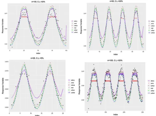
Each panel in Fig. 1 presents a single realization of simulated censored and uncensored observations and therefore, two different curves. A cutoff point is deter-mined for each simulation setting, and response observations are then censored according to this cutoff value. Hence, a nonparametric estimation of the regression functions in the case of right-censored data can be obtained via smoothing meth-ods using the iterated response variable stated in the imputation algorithm. The out-comes from this simulation study are presented in the following tables and figures.
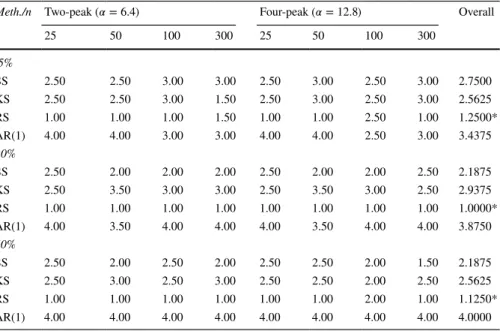
Table 1 displays the results for a minimal censoring level (5%). When the perfor-mance measures are inspected, it is shown that the three smoothing methods have considerable results, which is expected at a low censoring level. In addition, Table 1 shows that the proposed methods work well compared to the AR(1) model, even at the lowest censoring levels. The best scores are indicated in bold color. Table 1 can
c = 𝜇 + 𝜎F −1(1 − 𝜂) √ 1− 𝜙2 √ 1− 𝜙2(n+1) Ct= Yt ( 1− I(Yt> c))+ c.I(Yt> c), t= 1, … , n;
be inspected from two perspectives. One is by the shapes of the function, and the other is by the sample size. In this study, to measure the strength of the smoothing methods against the fluctuations in the function, two and four-peaked functions are used, and these peaks are censored by a determined detection limit. In this case, all of the obtained outcomes are presented in Tables 1, 2 and 3. When the censoring level is low and all the results are considered, KShas the highest number of colored scores (20/40), followed by. RS(19/40) and SS(15/40). Numbers in parentheses rep-resent the number of bold scores out of the total combinations. Note that usually, the values of KSand SS are close or equal in all three tables. When results are exam-ined in terms of sample sizes, for small samples, RS appears more efficient than the others. For medium samples (n = 50 and n = 100), KS and SS have reason-able results, and in large samples, SS performs the best. When the results are ana-lyzed in terms of spatial variation, it is clear that most of the methods’ performance decreases when fluctuation is increased, but the results are still satisfactory. The methods can be interpreted as being resistant to these kinds of fluctuations. How-ever, the RS shows a difference in modeling the multi-peak function. This result is not unexpected because RShas some advantages in knot selection. These results can easily be observed in Figs. 2 and 3.
In Table 2, the effect of the censoring level can be seen distinctly when compared with Table 1. All of the performance measures increased. In general, RS (22/40) showed better results than KS and SS. The results for the others were (18/40), (16/40), and (1/40) for KS, SS , and AR(1) , follow RS respectively. Surprisingly, although RS is last at a low censoring level, it is the best when the censoring level increases. This result might be worth examining further. RS is possibly better in esti-mating censored time-series in comparison with KS and SS. As expected, RS is at
Fig. 1 The panels show the censored and uncensored time-series observations from functions simu-lated under varying conditions: a for n = 25 and 𝜂 = 5% ; b for n = 50 and 𝜂 = 20% ; c for n = 100 and 𝜂 = 40% ; d for n = 300 and 𝜂 = 20%
Table
1
R
esults based on 1000 simulated sam
ples wit
h all sam
ple sizes (n) and r
eg ression functions f or censor ing le vel 𝜂 = 5 % 𝜂 =5% Tw o-peak ( 𝛼 = 6 .4 ) Four -peak ( 𝛼 = 1 2 .8 ) n Me th. MSE MAPE KL -N IQR RSE RAE MSE MAPE KL -N IQR RSE RAE 25 SS 0.0619 0.0233 0.6473 4.3347 4.9430 1.4773 0.0795 0.0244 0.9499 4.3744 5.9363 1.9842 KS 0.0569 0.0233 0.6473 4.3346 4.9421 1.4573 0.0806 0.0244 0.9499 4.3744 5.9363 1.9842 RS 0.0561 0.0225 0.6329 4.3332 4.9546 1.4656 0.0766 0.0213 0.9510 4.3495 5.9286 1.8591 AR(1) 0.0997 0.0299 0.8160 4.6913 5.1160 2.2279 0.1967 0.0738 1.0730 4.5342 6.1395 2.1820 50 SS 0.0390 0.0201 0.8849 3.2515 4.5260 0.9229 0.0463 0.0225 0.9017 3.3343 4.8751 1.6415 KS 0.0388 0.1701 0.8851 3.2515 4.5258 0.9138 0.0412 0.0225 0.9015 3.3343 4.8576 1.6402 RS 0.0384 0.0202 0.8849 3.2545 4.4417 0.9108 0.0463 0.0227 0.0966 3.3683 4.8705 1.6451 AR(1) 0.0629 0.0263 0.9140 3.5882 4.8246 1.6942 0.1794 0.0449 1.0222 0.7765 0.2014 0.4758 100 SS 0.0318 0.0201 0.8110 3.2237 3.4531 0.8448 0.0426 0.0209 0.6699 3.3041 4.5336 1.5548 KS 0.0317 0.0201 0.8092 3.2229 3.4387 0.7814 0.0375 0.0209 0.6702 3.3041 4.5336 1.5543 RS 0.0319 0.0203 0.8060 3.2244 3.4596 0.8144 0.0425 0.0192 0.5789 3.2975 4.5420 1.7252 AR(1) 0.0623 0.0264 1.4669 3.5937 3.8448 1.1077 0.0668 0.0265 0.6594 3.6561 4.7912 1.8374 300 SS 0.0253 0.0193 0.7263 3.1228 3.3888 0.7387 0.0357 0.0207 0.5219 3.2990 4.4518 1.3033 KS 0.0255 0.0198 0.7228 3.1333 3.3356 0.7612 0.0349 0.0209 0.5220 3.2990 4.4851 1.4740 RS 0.0265 0.0196 0.7559 3.1349 3.3733 0.7571 0.0362 0.0209 0.5543 3.2990 4.4211 1.3033 AR(1) 0.0421 0.0204 0.8728 3.4943 3.4780 0.8286 0.0494 0.0220 0.6981 3.5167 4.6407 1.6874
Table 2 Outcomes fr om t he simulated e xam ples f or all sam
ple sizes and r
eg
ression functions under t
he censor ing le vel 𝜂 = 2 0 % 𝜂 =20% Tw o-peak ( 𝛼 = 6 .4 ) Four -peak ( 𝛼 = 1 2 .8 ) n Me th. MSE MAPE KL -N IQR RSE RAE MSE MAPE KL -N IQR RSE RAE 25 SS 0.0954 0.0319 1.3247 5.4668 4.2788 2.4400 0.1145 0.0327 1.4425 5.5434 4.3633 2.4741 KS 0.0936 0.0319 1.3247 5.4668 4.2788 2.4400 0.0973 0.0326 1.4426 5.5434 4.3633 2.4553 RS 0.0954 0.0309 1.3413 5.4593 4.2533 2.4611 0.1148 0.0321 1.4450 5.5404 4.2676 2.4501 AR(1) 0.1533 0.0402 1.4999 5.7280 4.3829 2.5312 0.2061 0.0549 1.4795 6.0372 5.1098 3.1600 50 SS 0.0821 0.0319 1.2459 5.3353 4.1207 2.2754 0.0917 0.0309 1.2740 5.3616 4.3292 2.3003 KS 0.0842 0.0319 1.2459 5.3353 4.1206 2.2752 0.0863 0.0309 1.2740 5.3616 4.3294 2.3003 RS 0.0821 0.0322 1.2443 5.3370 4.1045 2.2539 0.0847 0.0312 1.3996 5.3565 4.2918 2.3001 AR(1) 0.0854 0.0360 1.6316 5.6642 4.3660 2.4191 0.1245 0.0512 1.8805 5.7260 4.6003 2.7809 100 SS 0.0781 0.0282 1.1382 4.3238 3.9762 1.3078 0.0811 0.0283 1.2148 4.4045 4.2123 1.6202 KS 0.0770 0.0282 1.1213 4.3143 3.9771 1.3078 0.0810 0.0283 1.2155 4.4045 4.2121 1.6129 RS 0.0786 0.0286 1.1654 4.3462 3.9647 1.3024 0.0801 0.0294 1.1840 4.4152 4.6194 1.6335 AR(1) 0.0820 0.0319 1.3224 4.5928 4.0322 1.6298 0.0920 0.0309 1.2609 4.7009 4.7711 1.8807 300 SS 0.0663 0.0262 1.0550 4.2410 3.8468 0.9462 0.0772 0.0270 1.1886 4.3952 4.1156 0.9994 KS 0.0510 0.0271 1.1938 4.2466 3.7708 0.9137 0.0747 0.0274 1.2050 4.3955 4.1175 1.0093 RS 0.0584 0.0312 1.1715 4.2719 3.8171 0.8229 0.0701 0.0269 1.1394 4.3946 4.1657 1.2175 AR(1) 0.0621 0.0315 1.1521 4.5691 3.8447 1.2020 0.0776 0.0289 0.9774 4.5594 4.2181 1.2360
Table 3 R esults fr om t he simulations f or all sam
ple sizes and all functions under t
he censor ing le vel 𝜂 = 4 0 % 𝜂 =40% Tw o-peak ( 𝛼 = 6 .4 ) Four -peak ( 𝛼 = 1 2 .8 ) n Me th. MSE MAPE KL -N IQR RSE RAE MSE MAPE KL -N IQR RSE RAE 25 SS 0.6103 0.0401 1.5129 5.6074 4.4741 2.7991 0.7524 0.0522 1.7860 5.6842 4.5460 3.3245 KS 0.6103 0.0401 1.5129 5.6074 4.4740 2.7990 0.7380 0.0522 1.7860 5.6842 4.5460 3.3245 RS 0.5052 0.0360 1.5088 5.5108 4.4671 2.7433 0.7152 0.0520 1.5669 5.6821 4.6201 3.3855 AR(1) 1.1668 0.0461 1.8998 5.6721 5.1503 3.2283 1.2367 0.0770 1.7596 5.8682 5.9158 4.6549 50 SS 0.2369 0.0383 1.4236 5.4201 4.3462 2.6952 0.4980 0.0466 1.4295 5.6210 4.4362 2.8977 KS 0.2459 0.0383 1.4138 5.4201 4.3462 2.6952 0.4794 0.0466 1.4296 5.6210 4.4362 2.8977 RS 0.2322 0.0391 1.4005 5.4209 4.3496 2.8020 0.4608 0.0399 1.2427 5.6222 4.4948 3.0864 AR(1) 0.7055 0.0466 2.6540 5.5936 4.6044 3.5285 0.7878 0.0426 1.4004 5.7232 5.1689 3.4166 100 SS 0.1572 0.0308 1.1952 5.3809 4.1388 1.4055 0.1422 0.0351 1.2690 5.5673 4.3855 1.9796 KS 0.1256 0.0309 1.1520 5.3811 4.1406 1.4056 0.1236 0.0351 1.2690 5.5672 4.3855 1.9794 RS 0.1087 0.0305 1.1076 5.3790 4.1089 1.3417 0.1105 0.0375 1.3153 5.5584 4.3643 1.9401 AR(1) 0.5591 0.0345 1.4197 5.5859 4.9682 2.3095 0.4870 0.0418 1.4081 5.7046 4.6060 2.2233 300 SS 0.0928 0.0271 1.0827 5.2767 4.1212 1.0666 0.0986 0.0273 1.1769 5.5246 4.1895 1.4907 KS 0.0912 0.0299 0.9848 5.2921 4.1216 0.9719 0.0968 0.0273 1.2139 5.5246 4.1840 1.4488 RS 0.0917 0.0294 0.9495 5.3022 4.0699 0.9535 0.0949 0.0275 1.2971 5.5154 4.1733 1.5250 AR(1) 0.3258 0.0354 1.6633 5.5989 4.3519 1.4004 0.3948 0.0288 1.5992 5.6029 4.5226 1.8259
the front in modelling the four-peaked function. Moreover, KS and SS have estimates for small and medium sample sizes that are more efficient, but for large samples, KS cannot match RSand SS.
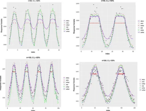
The results of Table 3 support the inferences gathered in examining Table 2. Namely, RS can model the censored time series better than the other two methods in the scope of this simulation study. It is observed that, when the censoring level increases, the performance of RSalso increases. Similar to other censoring levels, RS and SS produce better results for large samples, and for medium samples, KS and SS both perform reasonably well. Note that AR(1) has the worst performance for almost all of the simulation configurations and that the, performance of AR(1) is unsatisfy-ing under heavy censorunsatisfy-ing levels, which is due to it beunsatisfy-ing a linear and parametric method, as displayed in Tables 1, 2 and 3 and Figs. 2 and 3. Also note that Figs. 2 and 3 show the fits from the smoothing methods and an the AR(1) model for some selected combinations, as defined in Tables 1, 2 and 3, and the graphically summa-rized results support the outcomes expressed in the tables.
Figure 2 The plots of simulated observations, right-censored data points, and fit-ted curves from an autoregressive nonparametric time- series model using a classi-cal AR(1) model and three smoothing methods for different simulation configura-tions. Red points (.) denote the censored points..
Figure 3 the same as Fig. 2 but for different combinations
Fig. 2 The plots of simulated observations, right-censored data points, and fitted curves from an autore-gressive nonparametric time-series model using a classical AR(1) model and three smoothing methods for different simulation configurations, with red points (.) denoting the censored points
Figs. 2 and 3 prove that the augmented method works well in estimating right-censored time series under different scenarios. The three smoothing methods per-form satisfactorily, which is further illustrated in Tables4 and 5. It is worth noting that even if the censoring rate increases, the imputed values are still closer to real observations. To inspect this simulation study, see the web application available at https ://ey13.shiny apps.io/right -cens-times eries /, which dynamically reacts to differ-ent combinations of sample size, censoring level, and spatial variation.
As indicated in Sect. 4, we considered four different criteria for evaluating the performance of the proposed methods in this paper. However, especially for the simulation experiments, it was shown that the scores obtained from IQR and MSE criteria are very similar. Consequently, paired Wilcoxon tests were used to deter-mine whether the difference between the median values of MSEs (or median val-ues of IQRs) of any two criteria was significant at the 5% level. For example, if the median MSE value of a method is significantly less than the remaining three, it will be ranked first. If the medianMSE value of a method is significantly larger than one of the methods but less than the remaining two, it will be ranked second, and so on ranked third. Methods having non-significantly different median values will share the same averaged rank. Note also that the method or methods having the smallest rank are superior. Similar interpretations can be made for the IQR criterion.
The Wilcoxon test results for IQR and MSE are given in Tables4 and 5. Note that Tables 4 and 5 are constructed from the averaged ranking values of IQRs and MSEs, respectively, according to Wilcoxon tests for each censoring level and sample size.
Wilcoxon test results for the remaining criteria ( MAPE, KL − N, RSE and RAE) are not provided here to save space. For given simulation configuration, RS appears to be better than KS and SS according to the results obtained by 1000 repetitions. The overall scores of the tables further show that RS has the smallest median values in terms of IQR and MSE criteria. The SS and KS give similar ranking points. Moreo-ver, as the level of censorship increases, the difference between the points of the models increases. Note also thatKS and SS generally have similar scores, but KS performs better. Lastly, according to, the overall Wilcoxon test rankings in Tables 4 and 5, AR(1) has performed the worst.
5.2 Efficiency Comparisons
In order to illustrate and compare the relative efficiencies of the methods based on censored data, the bar charts of relative efficiencies computed from RE values are displayed in Fig.4. It is clearly shown that efficiencies ensure the outcomes in Tables 1, 2 and 3. As explained above, smaller efficiency values indicate a more efficient method. If Fig. 4 is inspected carefully, one can conclude that the KS has smaller values for small samples and low censoring levels, but when the censor-ing level begins to increase, the efficiency values of the RS decrease, which means the RS’s performance improves. The SS provides stable performance throughout the simulation experiments.
As seen in Fig. 4, efficiency values of the KS method are smaller than 1 for all censoring levels and sample sizes. Hence, KS method is more efficient than the other
Table 4 Averaged Wilcoxon test ranking values based on IQR criterion for the four methods under each sample size and censoring level
* denotes the best score
Meth./n Two-peak ( 𝛼 = 6.4) Four-peak ( 𝛼 = 12.8) Overall
25 50 100 300 25 50 100 300 5% SS 2.50 3.50 3.50 3.00 2.50 3.00 2.00 2.00 2.7500 KS 2.50 2.00 2.00 1.50 2.50 3.00 1.00 1.00 1.9375 RS 1.00 1.00 1.00 1.50 1.00 1.00 3.50 3.00 1.6250* AR(1) 4.00 3.50 3.50 3.00 4.00 3.00 3.50 4.00 3.5625 20% SS 2.50 3.00 2.50 3.00 2.50 1.00 3.00 3.00 2.5625 KS 2.50 2.00 1.00 1.50 2.50 2.00 2.00 2.00 1.9375 RS 1.00 1.00 2.50 1.50 1.00 3.00 1.00 1.00 1.5000* AR(1) 4.00 4.00 4.00 4.00 4.00 4.00 4.00 4.00 4.0000 40% SS 2.50 3.00 2.50 3.00 2.50 2.00 2.50 3.00 2.6250 KS 2.50 2.00 2.50 2.00 2.50 2.00 2.50 1.50 2.1875 RS 1.00 1.00 1.00 1.00 1.00 2.00 1.00 1.50 1.1875* AR(1) 4.00 4.00 4.00 4.00 4.00 4.00 4.00 4.00 4.0000
methods. When KS, RS, and SS are compared to the benchmark AR(1), it is shown that the RE values obtained from AR(1) increase. This means that AR(1) has the worst efficiency in terms of SMSE values.
6 Real‑Data Studies
6.1 Cloud‑Ceiling Data
This section more explicitly examines the estimation performances of the three smoothing methods for right-censored time-series data by modeling cloud-ceiling data. Cloud-ceiling data were collected hourly by the National Center for Atmos-pheric Research (NCAR) in San Francisco throughout March 1989. A dataset of
Table 5 Averaged Wilcoxon test ranking values based on MSE criterion for the four methods under each sample size and censoring level
* denotes the best score
Meth./n Two-peak ( 𝛼 = 6.4) Four-peak ( 𝛼 = 12.8) Overall
25 50 100 300 25 50 100 300 5% SS 2.50 2.50 3.00 3.00 2.50 3.00 2.50 3.00 2.7500 KS 2.50 2.50 3.00 1.50 2.50 3.00 2.50 3.00 2.5625 RS 1.00 1.00 1.00 1.50 1.00 1.00 2.50 1.00 1.2500* AR(1) 4.00 4.00 3.00 3.00 4.00 4.00 2.50 3.00 3.4375 20% SS 2.50 2.00 2.00 2.00 2.50 2.00 2.00 2.50 2.1875 KS 2.50 3.50 3.00 3.00 2.50 3.50 3.00 2.50 2.9375 RS 1.00 1.00 1.00 1.00 1.00 1.00 1.00 1.00 1.0000* AR(1) 4.00 3.50 4.00 4.00 4.00 3.50 4.00 4.00 3.8750 40% SS 2.50 2.00 2.50 2.00 2.50 2.50 2.00 1.50 2.1875 KS 2.50 3.00 2.50 3.00 2.50 2.50 2.00 2.50 2.5625 RS 1.00 1.00 1.00 1.00 1.00 1.00 2.00 1.00 1.1250* AR(1) 4.00 4.00 4.00 4.00 4.00 4.00 4.00 4.00 4.0000
Fig. 4 The column chart provides the relative efficiencies from the smoothing methods SS, KS, RS and AR(1)
716 observations was formed. The scale of the data was originally 100 feet, but here, a logarithmic transformation was made. It is visualized in Fig. 5. As men-tioned at the beginning of this paper, sometimes a measurement tool has a detec-tion limit. For this data, this limit is 12,000 feet (4.791 in log-transformed data); therefore, this time series is considered to be right censored. This means that each observation that is larger than the detection limit is censored. In the dataset, 293 observations are censored, and consequently, the censoring rate is 41.62%.
In Fig. 5, the points in red represent the censored observations. The follow-ing tables and figures summarize the findfollow-ings of the three smoothfollow-ing methods for estimating right-censored time series. Note that the imputation method can also provide an advantage in estimating censored data when there is no detection limit in the process of obtaining the data.
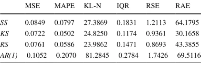
The performance measures for the three smoothing methods and the naïve AR(1) model, are presented in Table 6. The method with the best performance is indi-cated in bold. In this case, the KS had reasonable results according to almost all performance measures, and the KS is likely the best method for this type of censored time-series data. However, one must note that the RS shows its superiority for both absolute and relative performance measures, but in the general framework, the KS dominated the other two methods, while the AR(1) gave the highest scores for all evaluation metrics. As previously mentioned, the first three criteria for the estimated models measure the absolute error and the last two illustrate the relative error. In Tabl 6, one clearly sees that the RS performs better than the SS according to the first three criteria, which are MAPE, KL − N , and IQR, and, when RSE andRAE are inspected, it is clear that the performance of the RS is better than the SS.
Figure 6 represents the estimated values for the nonparametric regression model for the three smoothing methods, with the bottom right of the figure show-ing the observed real data versus augmented data points. The figure shows that the three methods all perform satisfactorily. When comparing the methods using
Fig. 5 Time plots of the log-transformed hourly cloud-ceiling height values with right-censored time series