Regressor-based adaptive infinite impulse response filtering

(1)

REGRESSOR BASED ADAPTIVE INFINITE IMPULSE RESPONSE

FILTERING

Carnegie Mellon University -

Pittsburgh, PA

15213

emrah@ece. cmu .edu

A B S T R A C T

To take advantage of fast converging multi-channel recursive least squares algorithms, we propose an adaptive IIR system structure consisting of two parts: a two-channel FIR adaptive filter whose parameters are updated by rotation- based multi-channel least squares lattice (QR-MLSL) algorithm, and an adaptive regressor which provides more reliable estimates to the original system output based on previous values of the adaptive system output and noisy observation of the original system output. Two different regressors are investigated and robust ways of adaptation of the regressor parameters are proposed. Based on extensive set of simulations, it is shown that the proposed algorithms converge faster to more reliable parameter estimates than LMS type algorithms.

1. THE R E G R E S S O R B A S E D IIR A D A P T I V E F I L T E R STRUCTURE

Emrah Acar

Dept. of Electrical and Computer Engineering

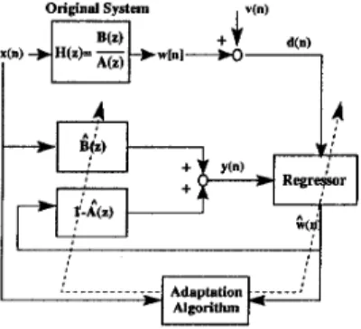
As shown in Fig. 1, in a typical adaptive filtering application, input, z(n), and noisy output, d ( n ) , of an unknown system are available for processing by an adaptive system to provide estimates, y(n), to the output of the unknown system as time progresses. In our investigation, the un-

Figure Common framework of IIR--y and IIR-Ka-nan known system or plant has an IIR model whose output can be compactly expressed as a function of its previous values

Orhan Arzkan

Dept. of Electrical Engineering

Bilkent University

Ankara, Turkey 06533

oarikan@ee. bilkent .edu.tr

and its input as:

N M

w ( n ) = C a j w ( n - j ) + C b i z ( n - I )

=e'$(?%),

(1)

j = 1 i=O

where

e

is the vector of direct form system parameters: T

-

e =

[ a ~ . . . a ~ b o . . . b ~ ] = [ aT bT

I T ,

(2) and $(n) is formed by the previous values of the output and the present and past values of the input:

T -

+(n) =

[

w ( n - 1).

. .

w ( n

-

N ) z ( n ) .

.

. z ( n

-

M )

3

=

[

w(n)T x(n)'

.

'

3

(3)

Unlike the FIR adaptation, in adaptive IIR filtering we are faced with the problem of deciding on the feedback signal used in the adaptation when we have noisy observa- tions of the actual system output. Hence, as shown explic- itly in Fig. 1, we use a regressor in the proposed structure which causally estimates the feedback signal based on the noisy output d(n) and the output of the adaptive filter y ( n ) ,

which is obtained as:

!An> = i?'(n)B(n) (4)

where &n) is the vector of estimated system parameters ([ &(TI)' G(n)'

]

') and $(n) is the vector of the regressor output, G(n), and the system input, z(n):

-

i ( n ) =

[

* ( n ) T x(n)'

1'.

_{( 5 )}

The performance of the adaptive filter heavily depends on how well the regressor, G ( n ) , provides estimates to the

actual system output w ( n ) . The two well known formulations of adaptive IIR filtering, namely the output error (OE) and the equation error (EE) formulations, correspond to two different types of regressors. In the OE Iformula- tion, the signal vector go(n) is described as: & ( n ) =

[

~ ( n ) ~ ~ ( n ) ~

]

'

which corresponds to a regressor whose output is the output of the adaptive filter. In t h e EE formulation the signal vector, &(n) is given as: &(n) =

[

d(n)T ~ ( n ) ~

]

which corresponds to a regressor whose

0-7803-4428-6198 $10.00 0 1998 IEEE

(2)

output is the noisy observation of the system output, d ( n ) = Since the least squares cost function of EE formulation is quadratic in terms of the parameter vector 6, fast converging recursive least squares techniques can be used in the adaptation. However, because of the additive measurement noise, w ( n ) , the converged parameter values are biased es-

timates of the actual system parameters [l]. In the OE formulation, the least squares cost function is not a quadratic function of the parameters. Hence, we are bound to use LMS type gradient descent techniques in the adaptation. When these LMS type adaptation algorithms converge to the global minima of the cost function, the obtained parameters are unbiased estimates of the cost function. Unfortu- nately, LMS type gradient adaptation methods not only converge slowly, but also may converge to a local minima of the cost surface.

In this work, we try to combine the desired features of

both OE and EE formalism in one formulation where the cost function is kept as a quadratic function of the parameters in order to use fast RLS techniques. As suggested in Fig. 1, this is achieved by choosing the adaptive filter as a two-channel FIR filter with inputs z ( n ) and 6 ( n

-

1).

Then, the corresponding weighted least squares cost function becomes:

w ( n )

+

w(n).

n

J(&

n) =

E(@)

-

eT(j(k))"X"-k, (6) k=l

which is a quadratic function of 6, because &n) is a fixed sequence- of vectors determined by the past>arameter estimates e(n - l ) , @(n

-

2),

. . .

,

@(O). Hence, efficient multi- channel FIR recursive least squares technigues can be used to obtain parameter estimates a t time n,

B(n),

as the min- imizer of J ( & n).

In the following section, two different types of regressors will be investigated in detail and corresponding recursive least squares adaptation algorithms will be presented.

2. PROPOSED REGRESSORS

2.1. IIR-y

The IIR-y regressor estimates the actual system output as

a convex combination of the noisy observations, d(n) and the adaptive filter output, y ( n ) :

where yn is the regression coefficient. The proper choice of

yn should be based on a measure of the reliability of the es-

timated system parameters. A significant deviation of y ( n )

from d ( n ) is an indication that the system parameters are not reliably estimated, and hence, yn should be set close to 1, so that equation error type adaptation should take place. On the contrary, if y ( n ) closely follows d ( n ) , then to reflect our level of confidence to the estimated system parameters, yn should be set close to 0, so that output error type adaptation should be performed. We propose to base the measure of reliability of the estimated system parameters on the statistical significance of the observed deviation between y ( n ) and d ( n ) sequences. For this purpose, one

way of choosing yn is based on weighted estimate of the expected energy of the error sequence e ( n ) = d ( n )

-

y ( n ) :

where AV is an exponential forgetting factor that can im- prove the performance of the estimator. In our investigation, we observed that the critical properties of the functional form between L(n) and yn are the boundary values I 1 and 12 such that yn = 0 if L(n)

< 11

and yn = 1

if L(n)

2

1 2 . In order to determine which values for 11

and 12 should be used, we investigated the expected values

of the L(n) for the cases of yn = 0 and yn = 1, which correspond to output and equation error adaptation cases, respectively. Assuming that

7%

= 0 and the estimated parameters have converged to the actual ones, the observed error sequence, e ( n ) , will be equal to w(n), the additive Gaussian observation noise. Hence, E { L ( n ) } will be a:,

the variance of v(n). Therefore, 11 is chosen as a:. Like- wise, when yn = 1, E{L(n)} is equal to the variance of

e ( n ) sequence for the EE formulation. Since the equation error, e E ( n ) is related to the output error, e o ( n ) as in [2]:

eE(n) = eo(n) -&'(n)eo(n), when v ( n ) is white noise, the variance of e E ( n ) can be written as: U: (1

+

zf,

ii:(n)),

at the time of convergence to true parameters. Hence, we propose to use:

N

11 = a:

,

I 2 = Ua,2(1+

Eh,?)

₍₉₎

i = l

where U

>

1 is introduced to avoid the convergence point of the equation error adaptation. For computational efficiency, the functional relation between L(n) and -yn is chosen as:

f 0

where K and p are two parameters providing some control

of the actual shape of the curve in between two boundaries

11 and 12. Fortunately, we observed that the behavior of the

algorithm is not so sensitive to these shape parameters. For each iteration, this regression algorithm requires ( N

+

11)

multiplications which is O ( N ) . 2.2. IIR-Kalman

Output of the IIR-Kalman regressor is an estimate of the actual system output obtained by using the Kalman filter on the following statespace model of the original system [3]:

(11) (12) w ( n

+

1) = Aw(n)

+

B x ( n )

d(n) = C w ( n + l ) + w ( n )

where C =

[

1 0

...

0

1.

Since the actual parameters are unknown in Eqn. ( l l ) , we can form

d

and

8

matrices by using the estimated parameters at time n. Then, we get

w ( n

+

1) = A(n)w(n)

+

,t?(n)x(n)

+

u ( n ) (13)

(3)

*K(n+lln) =

[

y(n) 2i)iT(n-l)

...

G K ( n - N N 1 )

1'

P ( n

+

lln) =

A(n)P(nln)A(n)T

+

R,(n)

Table 1: Equations of IIR-Kahan State Estimator

where u ( n ) is introduced as an additional noise term to the system dyqamics to p x o u n t for the approximations in

d

and

B

by d(n) and B ( n ) , which are equal to:

Since the approximations in d(n) and B ( n ) are only limited to the first row, the additional process noise u(n) is:

u(n) =

[

u(n) 0

...

0

1'.

(15)

Application of the Kalman filter on the approximated model requires the covariance matrices R,(n) and R,(n) of ~ ( n ) and v ( n ) , as well as an initial estimate to the state vector

w(0) and the variance of the initial system error

R,(O).

The

R,

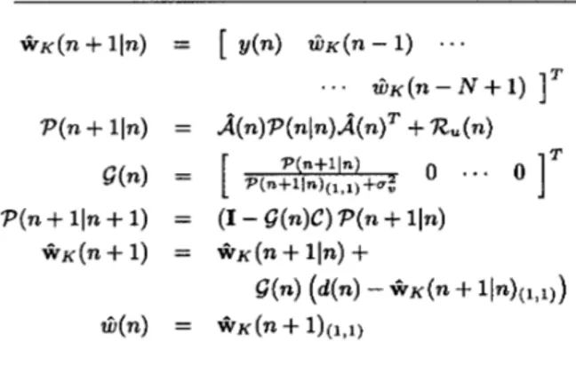
( n ) can be determined by the sample variance of u(n) for which a robust way is presented in [4]. The steps of the cor- responding Kalman estimator are given in Table 1, where

d(n), B(n), *(n) are defined in Eqns. (14), (5) and the no-

tation of ?1,1) is used to denote the first diagonal entry of

the matrix

7.

Note that the output of the regressor G ( n )

is the first entry in the estimated state vector + ~ ( n

+

1)

and also the a-priori state estimate + ~ ( n + l l n ) is obtained efficiently by using the output of the adaptive filter and the previous states of the Kalman filter. For each iteration, the Kalman regressor requires ( 3 N 2

+

2N) multiplications,

hence it is O ( N 2 ) .

The required two-channel FIR adaptation can be efficiently performed by using QR-MLSL algorithm which is a rotation-based multi-channel least squares lattice algorithm with many desired features [5]. For each update, this algorithm requires O(4N) multiplications. The required di-

rect form parameters for the Kalman regressor can be com- puted by using standard mapping rules between lattice and direct form parameters [5].

3. SIMULATION EXPERIMENTS

In the following simulations, the adaptive filters are "all- zero" initialized and reported system identification results are the ensemble average of 50 realizations. The proposed

algorithms are compared with two descent type IIR adaptation algorithms CRA [6] and BRLE [2], as well as with

the extended Kalman filter (EKF) algorithm (which is an O ( N 2 ) algorithm presented in [4]).

3.1. Simulation Example 1

The system to be identified is chosen as in [2]:

1

-

1.7e-l

+

0 . 7 2 2 5 . ~ ~ ' ' H ( z ) =

The input is a unit-variance white Gaussian process. The output noise, v ( n ) , is chosen as white Gaussian. ou is var- ied to investigate the sensitivity of the performance of the algorithms to the level of SNR.

In Fig. 2, the squared norms of the parameter error vectors, ee(n) =

e

- e(n) are plotted. o,, is set to 0.5. The forgetting factor, X of the QR-MLSL algorithm is chosen

as 0.999, and the parameters of the regressor subsystem of Eqns. (9) and (10) are chosen as X u = 0 . 9 , ~ = 1 , n =

0.7, U = 2. For the IIR-Kalman regression algorithm, the initial variance estimate, CE(0) is chosen as unity. In or- der to better resolve the early convergence behaviors of the compared algorithms, a logarithmic time axis is used in Fig. 2. As seen in this figure, the proposed algorithms have converged to an error level of -10 dB earlier than the 1000th sample, but the CRA and BRLE algorithms converge to the same error level at about 40000th sample. The EKF algorithm, performing the best, converges to -20 dB at around

50000th sample. Here, the same step-size of 0.0005 is used for the CRA and BRLE algorithms. As recommended in [2]

and [6], the composition parameter 7 for CRA is chosen as

0.9, and the remedier parameter of BRLE, ~ ( n ) is chosen In this example, conventional equation and output error (EE and OE) adaptation converged to error levels of -7 dB and 5 dB respectively, which are significantly higher than those of compared algorithms here. Therefore, as ini- tially expected, the performance of the regressor based RLS approaches can be better than both the EE and OE formulations.

We repeated this experiment at different noise levels and reported the obtained Ilee(n)1I2 results in Table 2. In this experiment, the best performing algorithm is found as the EKF algorithm. However, EKF requires an order more multiplications than IIR-7 algorithm. As seen from these results, at high SNR (low levels of U,,), LMS type algo-

rithms converge to lower error levels. However, as the SNR decreases (high values of CT,,) the proposed algorithms start

providing closer or better results than LMS type algorithms, which is an important advantage in many practical applications. Note that, the tabulated results correspond to the error levels at the 5000th sample for the proposed algorithms and 50000th samples for the EKF, CRA and BRLE algo- rithms. Since, in many important applications, the speed of convergence is critical, the proposed algorithms provide a good trade-off between error levels and the speed of convergence even at high SNR. Also, IIR-y provides comparable results to IIR-Kalman although it requires an order less number of multiplications.

as min(ll&n)

Illlleo

(4

II

7 1).

(4)

p

-0.10 0.25 0.50 1.00

ow

I

IIR-7 IIR-Kalman EKF CRA BRLE

0.05

I

-74.57 -82.25 -74.55 -84.97 -77.38 -50.92 -56.29 -69.49 -62.50 -55.72 -24.19 -27.18 -38.88 -32.16 -28.38 -10.27 -10.90 -21.27 -11.31 -10.23 -1.40 0.40 -5.62 3.61 3.53

Figure 2: Squared norm of parameter error (Example I )

3.2. Simulation Example 2

In this example, an abruptly changing system is selected with the time-varying transfer function:

0.2759+0.5121z-1+0.5121z-2+0.2759~-3 1-0.001~- 4-0.65462- -0.07752- l+O.OO1z-l +0.6546ra + 0 . 0 7 7 5 ~ ~

<

500 0.7241+0.487912-1+0.48792r-2+0.72413x-3 2 500 (17)

The input sequence is chosen similar to the previous example. The output noise .).( is chosen as a zero-mean white Gaussian noise with a variance of 0.25. The stepsize of CRA and BRLE algorithms is set to 0.01. The composition parameter, y of CRA is set to 0.5, and the remedier param- eter, ~ ( n ) of BRLE is determined as in the fist example. The forgetting factor of the proposed algorithms is set to

0.99 for a better tracking of the variations in the system pa-

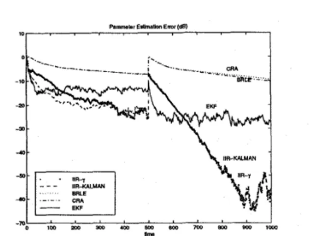
rameters. For IIR-Kalman algorithm, initial variances are chosen as unity. The parameters of IIR-7 in Eqns. (9) and (10) are chosen as A,, = 0 . 9 5 , ~ = 1, n = 0.3, U = 5. EKF is also initialized with all-unit variances. The squared norm of parameter errors Ilee(n)112 is shown in Fig. 3. As seen from these results, both CRA and BRLE, whose performance are

very close to each other, are outperformed by the proposed algorithms. IIR-7 and IIR-Kalman have the best performance where EKF algorithm has converged to a higher error level. Again, at an order less amount of multiplications, IIR- y provides comparable results to IIR-Kalman.

0

-10

Figure 3: Squared norm of parameter error (Example 2)

system structure is proposed. Two different regressor algorithms, requiring O ( N ) and O ( N 2 ) number of multiplica- tions respectively, are proposed t o provide reliable estimates to the system output. Based on extensive set of simulations, it is found that for timeinvariant systems, the proposed algorithms not only converge faster than LMS type algorithms, but also provide more reliable parameter estimates a t low SNR. Additionally, in the simulation of the systems with abrupt changes, it is observed that the proposed regressor based adaptation algorithms establish faster convergence t o lower error levels, outperforming BRLE, CRA and EKF.

5. REFERENCES

[l] T. Soderstrom and P. Stoica, System Identification. En-

glewood Cliffs, NJ: Prentice Hall, 1988.

[2] J. Lin and R. Unbehauen, “Bias-remedy least mean square equation error algorithm for IIR parameter recursive estimation”, IEEE Trans. o n Signal Processing, vol. 40, pp. 62-69, Jan. 1992.

[3] C. Chui and G. Chen, Kalman Filtenng with Real-Time AppZications. Berlin: Springer-Verlag, 1991.

[4] E. Acar, “Regressor Based Adaptive Infinite Impulse

Response Filtering”, Master’s thesis, Dept. of Electrical Engineering, Bilkent University, Ankara, Turkey, 1997.

[5] B. Yang and J. Bohme, “Rotation-based RLS algo-

rithms: Unified derivations, numerical properties, and parallel implementations”, IEEE Trans. o n Signal Pro-

cessing, vol. 40, pp. 1151-1167, May 1992.

[6] J. Kenney and C. Rohrs, “The composite regressor algorithm for IIR adaptive systems”, IEEE R a n s . o n Signal Processing, vol. 41, pp. 617-628, Feb. 1993.

4. CONCLUSION

In order to use fast recursive least squares adaptation algorithms in adaptive IIR filtering, a regressor based adaptive