MEASUREMENT OF FINANCIAL INTEGRATION: THEORY REVIEW AND A NEW APPROACH TO EULER TEST
A Master’s Thesis by HAKAN ER Department of Economics Bilkent University Ankara September 2009
MEASUREMENT OF FINANCIAL INTEGRATION: THEORY REVIEW AND A NEW APPROACH TO EULER TEST
The Institute of Economics and Social Sciences of
Bilkent University
by
HAKAN ER
In Partial Fulfillment of the Requirements for the Degree of MASTER OF ARTS in THE DEPARTMENT OF ECONOMICS BİLKENT UNIVERSITY ANKARA September 2009
I certify that I have read this thesis and have found that it is fully adequate, in scope and in quality, as a thesis for the degree of Master of Arts in Economics
--- Asst. Prof. Dr. Taner Yiğit Supervisor
I certify that I have read this thesis and have found that it is fully adequate, in scope and in quality, as a thesis for the degree of Master of Arts in Economics.
---
Assoc. Prof. Dr. Fatma Taşkın Examining Committee Member
I certify that I have read this thesis and have found that it is fully adequate, in scope and in quality, as a thesis for the degree of Master of Arts in Economics.
---
Assoc. Prof. Dr. Başak Tanyeri Examining Committee Member
Approval of the Institute of Economics and Social Sciences
--- Prof. Dr. Erdal Erel Director
iii ABSTRACT
MEASUREMENT OF FINANCIAL INTEGRATION: THEORY REVIEW AND A NEW APPROACH TO EULER TEST
Er, Hakan
M.A., Department of Economics Supervisor: Asst. Prof. Dr. Taner Yiğit
September 2009
An extension of the Euler test in which the real interest rate differential is explained by the growth rate of real consumption of the domestic and the foreign country, and new proxies developed to measure real interest rate differential instead of ex post real interest rate constitute the backbone of this paper. The proxies are obtained directly from the real economic variables that try to overcome the difficulty of measuring unobservable ex post real interest rates, which, by nature, may contain monetary shocks, and varies considerably according to the reference nominal interest rates and baskets that measures the price developments. In one of the above-mentioned proxies, a new factor trying to capture the effect of human capital growth developments on real interest rates has been included. After constructing these new proxies, the validity of the extended Euler test has been checked for 11 OECD countries and the level of these countries’ integration to the world has been tested by taking United States as the foreign country.
iv ÖZET
FİNANSAL ENTAGRASYON ÖLÇÜMÜ: TEORİK DEĞERLENDİRME VE EULER TESTİNE YENİ BİR YAKLASIM
Er, Hakan
Mastır, Ekonomi Bölümü
Tez Yöneticisi: Yrd. Doç. Dr. Taner Yiğit
Eylül 2009
Reel faiz oranı farklarının yurtiçi ve yurt dışı reel tüketimdeki büyüme oranıyla açıklandığı Euler testinin bir uzantısı ve ex post reel faiz oranları yerine reel faiz oranı farklılıklarını açıklamaya çalışan yeni göstergeler bu çalışmanın temelini teşkil etmektedir. Bu göstergeler gözlemlenemeyen, doğası gereği parasal şokları içerebilen ve referans nominal faiz oranlarına ve fiyat değişimlerinin ölçüldüğü sepete göre oldukça çok değişebilen expost reel faiz oranlarının ölçülmesindeki zorluğun üstesinden gelmek için doğrudan reel ekonomik değişkenlerden elde edilmiştir. Bu göstergelerden birinde beşeri sermaye büyümesindeki gelişmelerin reel faiz oranlarına etkisini kapsamaya yarayan yeni bir faktör eklenmiştir. Bu yeni göstergelerin oluşturulmasından sonra genişletilmiş Euler testinin geçerliliği 11 OECD ülkesi için kontrol edilmiş ve ülkelerin dünyaya entegrasyonu yabancı ülke olarak ABD’nin esas alınması ile test edilmiştir.
Anahtar Kelimeler: Euler Testi, Finansal Entegrasyon
v TABLE OF CONTENTS ABSTRACT...iii ÖZET... iv TABLE OF CONTENTS... v LIST OF TABLES ... vi
LIST OF FIGURES ...vii
CHAPTER I: INTRODUCTION... 1
CHAPTER II: THEORIES FOR FINANCIAL INTEGRATION ... 5
2.1 Correlations Between Saving and Investment Ratios ... 5
2.2 Deviations from Interest Parity ... 8
2.2.1 (Ex ante) Uncovered Interest Rate Parity (UIP) ... 8
2.2.2 Covered Interest Rate Parity (CIP) ... 9
2.2.3 Real Interest Rate Parity (RIP)... 10
2.3 Cross-Country Consumption Growth Correlations... 12
CHAPTER III: THEORETICAL AND EMPIRICAL MODEL ... 17
CHAPTER IV: DATA ... 22
CHAPTER V: ESTIMATION RESULTS... 24
5.1 Individual Time Series Results ... 24
5.2 Panel Data Results... 30
CHAPTER VI: CONCLUSION ... 33
SELECT BIBLIOGRAPHY ... 35
APPENDIX A ... 39
vi
LIST OF TABLES
Table 1: Correlation Matrix of the Independent Variables ... 39
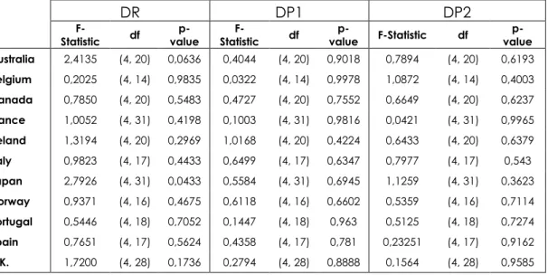
Table 2: White Heteroskedasticity Test for the 3 Competing Models... 39
Table 3: Serial Correlation LM Test (with Two Lags) for 3 Competing Models... 40
Table 4: HAC Corrected Estimation Output with Dependent Variable DR ... 40
Table 5: HAC Corrected Estimation Output with Dependent Variable DP1... 41
Table 6: HAC Corrected Estimation Output with Dependent Variable DP2... 41
Table 7: Sign Check for the 3 Competing Models... 42
Table 8: The test for presence of Financial Integration based on Wald Test... 42
Table 9: Stability and Specification Tests for the Model with Dep. Variable DP2 ... 43
Table 10: Panel Estimation Results for Three Competing Models... 43
vii
LIST OF FIGURES
Figure 1: (DRIR=DP2) (France) Residual vs. Fitted Value... 45
Figure 2: (DRIR=DP2) (France) Residual vs. Residual (-1) ... 45
Figure 3: Correlogram-Q-Statistics for DRIR=DP2 (France)... 46
Figure 4: (DRIR=DP2) (France) Res. vs. Res (ar(1)) ... 46
1
CHAPTER I
INTRODUCTION
The last decade has been characterized by financial liberalization process that has led several industrialized and developing countries to dismantle or drastically reduce the restrictions on international capital mobility. In the member countries of European Monetary System, capital controls were gradually dismantled during 1980`s and abolished by 1990. In several developing countries, barriers to international capital movements are being reduced, as domestic investors are allowed to purchase foreign assets and non-residents to invest in domestic financial markets (Feretti, 1998). On the other hand, in Furstenberg (1998), it is noted that while capital flows across the borders exceeds one trillion dollars a day, and despite the increased number of countries that has access to world capital markets, the number is only 56 out of 180 countries that has membership to IMF. Therefore, Bayoumi and MacDonald (1995) emphasize that measuring the actual level of financial integration through the world is, therefore, proved to be much more difficult. Moreover, the progress in this literature is spurred by the failure of systematic predictions, which cannot explain the level of financial integration properly. This situation invites new approaches to the topic, preserving its popularity.
2
In this study I will develop a variation of “Cross-Country Consumption growth correlations” model since the approach has several attractive features when compared to the competing models. First, the underlying theory in these types of studies is stronger than the saving-investment correlations. Furthermore, since consumption is the ultimate goal of the economic activity, constructing the test of financial integration on economic welfare is more robust than making comparisons on nominal or real interest rates.
The classical model of “Cross-Country Consumption Growth Correlations” has been modified in two steps:
1. Theoretically, the result in Lemmen and Eijffinger (1998) has been replicated by an aggregate output function including human capital, in which the real interest rate differentials can be explained by the growth rate of consumption of the domestic and the foreign country
2. In addition, two new competing proxies for real interest rate differential calculated by using real variables of the economies, have been employed in addition to ex post real interest rates, which are:
a. The differences of “marginal productivity of physical capital minus capital depreciation rate” calculated for the domestic and the foreign country
b. The differences of “Marginal productivity of physical capital minus capital depreciation rate plus the human capital growth rate” calculated for the domestic and the foreign country
The first step provided a convenient way to get testable restrictions implying that the previous periods’ consumption growth rate has no explanatory power on real
3
interest rate differentials, as it is the case in Lemmen and Eijffinger (1998). In the second step, I try to overcome the difficulty with measuring the real interest rate since using different references with different horizons for interest rates and different inflation measures using different baskets lead to considerable variation in calculated ex post real interest rates. Therefore, I have developed two proxies for the real interest rate by using only real variables. In the first proxy, in order to find the marginal productivity of capital, I used the capital share in real production and output capital ratio. The first proxy for the real interest rate was then adjusted for human capital growth rate by adding a factor that relates human capital growth rate. The idea in this adjustment is that, for the investments, possible returns should also be related to the human capital growth rate of the whole economy and there should be a premium on real interest rates if this factor has been taken into account.
In addition to these extensions I have used calibrated values for relative risk aversion constants. In Obstfeld (1989), Lemmen and Eijffinger (1998) and in similar studies for testing financial integration by Euler tests, the analyses have been carried out by taking the same relative risk aversion constants for all countries in consideration. What is more, the tests have been repeated for various values of relative risk aversion (e.g. 0.25, 0.75, 1, 1.5, and 2). I think that using calibrated values would create more reasonable results for these types of tests.
The structure of the paper is as follows: Part II will give a brief review of theories for financial integration. Part III will present the theoretical and the empirical model. Part IV will explain the nature and the sources of data that will be utilized to test the theory developed in this study. Part V will be a demonstration of empirical results for time series and panel data. Part VI shall give a summary and
4
interpretation of the results, in addition my conclusions and the possible extensions of my approach.
5
CHAPTER II
REVIEW OF THE THEORIES FOR FINANCIAL
INTEGRATION
When the past studies are examined in an eclectic way, the most influential approaches to the measurement of international financial integration might be “Correlations Between Saving and Investment Ratios”, “Deviations from Interest Parity” and “Cross-Country Consumption Growth Correlations”. Therefore, in this part of the paper a brief review and a discussion of the literature on these three measurement approaches for financial integration is presented.
2.1 Correlations between Saving and Investment Ratios
Starting from Feldstein and Charles Horioka’s seminal paper in year 1980, the measurement of international financial integration by the correlations between saving and investment ratios became important in the relevant literature. The basic idea underlying this approach was, if the capital were actually perfectly mobile, a shortage in national saving in one country should have been readily made up by borrowing from abroad at present world interest rate. Therefore a shortage in the national saving should not crowd out the domestic investment. Since the focus of approach is towards examining the volume of capital flows, the test of financial
6
integration based on the F-H criterion fits into the quantity approach to the financial integration (Feldman, 1986).
The Feldstein-Horioka definition requires that the domestic country’s real interest rate is always tied to the world real interest rate1. In this theory, saving and investment is explained by real interest rate rather than nominal interest rate. As an additional assumption, any and all determinants of a country’s rate of investment other than real interest rate are uncorrelated with its national saving. Investment rate is given by the equation:
i u i r b a i Y I + × − =
where a and b are constants, I is the level of capital formation in the economy, Y is the national income, r is the domestic real interest rate, and u represent the all other factors that determine the rate of investment. Feldstein and Horioka (1980) made a regression against the national saving rate as:
i v i Y NS B A i Y I + × − =
where A and B are constants, NS is the private saving minus the budget deficit. Their regression based on the above model upset the conventional wisdom in 1980. Under their null hypothesis of perfect capital mobility, B2 should be zero for small scaled countries’; on the other hand, for large countries B should approximate the country’s share of the world capital stock. Their estimation for the B value was 0.887( =σ 0.074)for the period 1960-74. The result was significantly different from zero and insignificantly different from one at 95 percent level of confidence. They
1 Therefore, the approach assumes “Real Interest Parity Condition” holds, which is simply
equalization of real interest rates because of international capital flows. Real interest parity condition is another approach for the measurement of International capital account openness and also told in this paper.
2
Maurice Obstfeld (1986) emphasizes that the least-square estimate of B is not a correlation coefficient, and there is no reason for it to be less than 1.
7
concluded in their paper that changes in countries’ rates of national saving had very large effects on their rates of investment and interpreted this result as evidence to the lack of high international capital mobility. There have been many criticisms about F-H that tried to bring objections econometrically. These criticisms may be divided into two main categories.
The main idea commonly agreed in the first category of studies is that national saving is endogenous, thus correlated with ui. Therefore, these studies
added more control explanatory variables in the regressions. Maurice Obstfeld (1986) argues that income and population growth may affect savings and investment. Norman Fieleke (1982), James Tobin (1983), Lawrence Summers (1988) and Tamim Bayoumi (1990) carried the “policy reaction” argument into the discussions by arguing that if the government respond endogenously to the current account imbalances with policies to National saving (public or private) in such a way to reduce the imbalances, national saving will again be endogenous to “policy reactions”. However, F-H were aware of the econometric endogeneity problem of national saving. To solve the cyclical endogeneity, they computed averages over a long enough period of time during which the business cycle effects are believed to disappear. To handle other sources of endogeneity they used demographic variables.
The main idea commonly agreed in the second category of studies is that, if domestic country is relatively large in the world markets, then real interest rate of the world economy will not be exogenous with respect to national saving ratio. This means that, if the national saving in this large country falls back, the world saving rate would increase and therefore saving in the domestic country as well as abroad
8
will decrease. These “large country” arguments have been made by Tobin (1983) and Robert Murphy (1984).
If the saving-investment regressions tests were a good means of testing the international financial integration, then we would have been observing coefficient B falling over time, since this point is one of the stylized facts in the global economic environment. Unfortunately, until recently, this observation cannot be proved by the evidence from the papers, which typically report before and after 19733 (Feldstein 1983; Alessandro Penati and Michael Dooley 1984; Obstfeld 1989).
2.2 Deviations from Interest Parity
Traditionally, interest parity conditions have been used to describe the integration between international financial markets. Since the focus is on returns, tests of international financial integration based on interest parity conditions fit into the price approach to financial integration (Feldman, 1986). In this context there are three parity conditions that are widely used for the measurement in literature: Uncovered Interest Rate Parity, Covered Interest Rate Parity and Real Interest Rate Parity. In this sub-section, firstly these three conditions will be examined, and then the literature for measurement of international financial integration through these conditions will be reviewed.
2.2.1 (Ex ante4) Uncovered Interest Rate Parity (UIP)
3 International financial integration was greatly accelerated after 1973 when US, Germany, Canada,
Switzerland and Netherlands removed capital controls. Therefore, this year is regarded as a benchmark for transformation to the capital openness.
4
Ex ante is Latin word for "beforehand". In models where there is uncertainty that is resolved during the course of events, the ex antes values (e.g. of expected gain) are those that are calculated in advance of the resolution of uncertainty.
9
According to UIP condition the foreign exchange market is in equilibrium when deposits of all currencies offer the same expected return. The condition that the expected returns on deposits of any two currencies are equal when measured in the same currency is called the (ex ante) interest rate parity condition. It can be formulated as: Ep d i d f s d f s e d f Es d i f i = + − + = / ) / / (
where ifdenotes foreign market’s interest rate, iddenotes domestic market’s interest
rate, e d f
Es / denotes expected exchange rate measured in domestic currency, sf/d
denotes spot exchange rate measured in domestic currency, Ep denotes expected premium of exchange rate measured in domestic currency.
2.2.2 Covered Interest Rate Parity (CIP)
The covered interest rate parity condition states that the rates of return on domestic deposits and “covered” foreign deposits must be the same. Or we can state the CIP condition as follows: The interest rate on foreign currency deposits equals the interest rate on domestic currency deposits plus the forward premium on domestic currency against the foreign currency. It can be formulated as follows
Fp i s s Fs i i d d f d f d f d f = + − + = / / / ) (
where ifdenotes foreign market’s interest rate, iddenotes domestic market’s interest rate, e
d f
Fs / denotes forward exchange rate measured in domestic currency, sf/d denotes spot exchange rate measured in domestic currency, Fp denotes forward premium of exchange rate measured in domestic currency.
10
2.2.3 Real Interest Rate Parity (RIP)
As the other interest parity conditions RIP states that real rates of return on domestic currency deposits and foreign currency deposits should be the same. We can shortly formulate this condition as follows:
d f
r
r =
One of the most appreciated studies on the interest rate differentials and their relations is Frankel (1992). In this study it is argued that the endogeneity of national saving is not an explanation for the anomalous results of Investment-Saving correlation studies. And adds that the most important reason for the anomalous results is “real interest parity condition” that is assumed to hold in investment-saving correlation models for international financial integration. He claims that real interest parity condition may not hold in all periods and concludes that if the domestic real interest rate is not tied to the foreign interest rate, then there is no reason to expect a zero coefficient in the saving-investment regressions5.
In Frankel (1991), the writer studies real interest rate differentials in the 1980’s for a panel of 25 countries. In some respects country-group comparisons of the measures of real interest differential variability fits a prior expectations about financial integration. Five closed low developed countries constitute the group with the highest variability, and five open Atlantic countries constitute the group with the lowest variability. However, the writer argues that there are some anomalous results when the real interest rate differential is taken as a measure of financial integration. For instance, although France had very strict capital controls during the 1980’s, when the real interest parity condition is used it appears to have a higher degree of capital
5
He supports his idea with the fact that, the real interest rate in the U.S. rose far above its trading partners in the early 1980’s.
11
mobility than Japan, the Netherlands, or Switzerland-countries that are widely known for their free capital controls. Moreover, in his study he finds that no country in question has a real interest rate differential equal to zero. In Frankel (1992), the writer asks the question “If barriers to capital mobility are so low among the major industrialized countries, why does it not show up in real interest differentials?” To give the answer he makes a decomposition of real interest differential into Country Premium and Currency Premium:
0 ) * ( ) ( ) * ( ) * * ( ) ( * 0 * * = ∆ − ∆ − ∆ + ∆ − + − − = ∆ − − ∆ − = = − = − ⇒ = e p e p e s e s Fd Fd i i e p i e p i r r r r r r (α) (β) where i and *
i are the domestic and foreign nominal interest rates, Fd is the forward
discount on the domestic currency, e
s
∆ is expected depreciation of the domestic currency, e
p
∆ is expected domestic inflation and e* p
∆ is expected foreign inflation.
The first term in the final decomposition denoted by α is covered interest differential and called country premium. In Frankel (1992), this terms is defined as “an unalloyed criterion for capital mobility” This term captures all barriers to integration of financial markets across all boundaries as transaction costs, information costs, capital controls, tax laws that discriminate by country of residence, default risk, and risk of future capital controls. The second term (exchange risk premium) and the third term (expected real depreciation) in the decomposition together constitutes currency premium (β). This term captures the differences in assets according to the currency which they are denominated, rather than in terms of political jurisdiction in which they are issued.
12
Frankel (1992) concludes that even for those countries that exhibit no substantial currency premium, as reflected in covered interest rate parity, there is still a substantial currency premium that drives real interest differentials away from zero. If real interest differentials are not arbitraged to zero, there is no reason to expect saving-investment correlations to be zero. In addition, according to the writer only the country premium has been eliminated in the international financial integration period, that is, covered interest differentials (unalloyed criterion for financial integration) are very small. But, the exchange rate variability leading currency premium remains, consisting of an exchange rate risk premium plus expected real currency depreciation. This means that, despite the equalization of covered interest rates, large differentials in real interest rates remain.
2.3 Cross-Country Consumption Growth Correlations
Among the benefits that are expected to result from international financial integration consumption smoothing and risk diversification are very important, the main aim in these types of tests is to measure the degree to which capital flows contribute to risk diversification and consumption smoothing. If the international financial integration is achieved, then the residents across countries will be able to use the similar financial instruments, using the same financial derivatives will lead testable restrictions on the co-movement of consumption growth rates. (Eijffinger and Lemmen, 2003, Volume I)
The Lucas criticism at 1970’s, argues that most macro-economic models are indeed based on static expectations, and inclusion of rational expectations results in more exact force of expressions. Loosely speaking, his criticism was that the
macro-13
economic models that depend on static econometric analyses cannot be used for policy arguments. These econometric regressions are only a picture for a given time, keeping all other policy arguments fixed. When we change the policies, the regression is already changed with its coefficients. Therefore, dynamic optimization models with rational expectations are better tools for macro-economic modeling and policy making purposes. Parallel to this trend, Obstfeld (1989) uses an inter-temporal dynamic optimization model with rational expectations for modeling consumption smoothing by: Maximize ∑∞ = − t ψ U(ct)] t ψ β
Ε[ subject to Budget Constraints
where Et[.] is conditional expectation based on time-t information, β<1 is a subjective discount factor, ct is consumption on date t, and the period utility function U(.) is strictly concave and differentiable.
The optimization gives:
(I) } 1 ) t (C ' U ) 1 t (C ' U β ) 1 t P t P )( t i {(1 t E × + = + + & (II) 1 1 1 1 1 × + = + + + } ) t * (C ' U ) t * (C ' U * β ) t P t X t P t X )( t i {( t E
where (I) and (II) are domestic and foreign consumer’s Euler equation respectively. To implement these Euler equations empirically, two strong assumptions are made: First, it is assumed that consumers within a country are alike with respect to endowments and preferences, so that the above equations can be tested using aggregate per capita consumption levels in the two countries; second, it is assumed that the marginal utility of consumption level c is given in both by '( )= − , >0
α
α
c c U
14
for the both countries; and Xt denote the home-currency price of foreign currency) 6. Euler equations and the assumptions just made lead to the following equations:
( ) ( ) ( ) ( *) 0 1 1 * * 1 * 1 1 1 = − = + + + + + + t t t t t t t t t t t t P X P X C C P P C C E α α η 0 ) ( ) ( ) / / ( ) ( * 1 * * 1 * 1 1 1 * 1 = − = + + + + + + t t t t t t t t t t t t P P C C X P X P C C E α α η
According to the equations E[ηt+1]=0 and E[ηt+1*]=0, discrepancies between ex post marginal rates of substitution are unpredictable on the basis of time-t information if everyone can trade the same nominally risk free home and foreign currency bonds. These conditions can be falsified empirically if any information known at time t-1 or earlier is useful in forecasting values of η or *
η
dated t or earlier. That is, past discrepancies of consumption do not have an importance to help forecast future discrepancies. Obstfeld (1989) estimates the regression equations of the following form for different values ofα
:∑ = − + + = N i i t i Vt t 1 0 γ η γ η & * 1 * * * 0 * ∑ = − + + = N i i t i Vt t γ γ η η
where Vt and Vt*are errors orthogonal to information dated t-1 or earlier. Therefore
we are testing the null hypotheses:
(I) H0:γ0 =γ1=...=γN =0 and (II) H0*:γ0*=γ1*=...=γN*=0
In the first one it is tested whether people in different countries equate ex ante marginal rates of substitution of present for future units of home currency through inter-temporal trading at the same home currency interest rate. In the second one it is
6
According to the writer there is no justification for the first assumption other than the practical alternatives, in addition writer emphasizes that the second assumption is consistent with the evidence.
15
tested whether people in different countries equate ex ante marginal rates of substitution of present for future units of foreign currency through inter-temporal trading at the same foreign currency interest rate.
According to the Bayoumi and MacDonald (1995) focusing on consumption has several attractive features. The underlying theory in these types of studies is stronger than the saving-investment correlations. In addition, since consumption is the ultimate goal of the economic activity, constructing the test of financial integration on economic welfare is more basic than making comparisons on nominal or real interest rates. One other advantage is that private nondurable consumption and the macroeconomic policy are normally uncorrelated, that is it is unlikely that they are in the same way.
In addition to consumption smoothing, the literature on international risk sharing and its potential welfare gains seems to be very promising development in the theory sense. Through open capital markets, firms and households can diversify away idiosyncratic country specific risks. With such an allocation, a country’s domestic private consumption is affected only by uninsurable global shocks, and has a co-movement with the world’s consumption patterns. Obstfeld (1994) develops a general method for analyzing international consumption co-movements when there is a cross border trade in assets. The paper mainly uses the regression of the form:
ε β
α + ∆ +
=
∆logCti . logCtw
This equation is the workhorse of the paper’s empirical study, and test of financial integration based on this equation asks if the coefficient of w
t
C
log
16
The coefficients in the regressions show that the coefficients are positive but smaller than one, implying a partial risk sharing among the world capital markets.
One of the reasons for the partial international risk sharing might be home equity bias. The main idea in this reasoning is that majority of the investors choose to invest most of their wealth at their home country and do not diversify their portfolios over different financial instruments in world. The home bias in equities was first documented by French and Poterba (1991) and Tesar and Werner (1995)
17
CHAPTER III
THEORETICAL AND EMPIRICAL MODEL
Since the theory behind cross-country consumption growth correlations is very strong and its aim is to make a test on the consumption, which is one of the main targets of the economic function and consistent data about which can be always accessible, I prefer to elaborate the theory about these tests and make empirical research by our new method and proxies for the variables.
For this purpose, I start with an inter-temporal dynamic optimization model, with aggregate output function including human capital, with rational expectations for modeling consumption smoothing:
Maximize ∑ ∞ = − − − 0 1 1 1 t t C t t E α α β subject to θ λ θ λ δ − − − − = − − + = + 1 . 1 . 1 . 1 ) 1 ( t L t H t K A t Y t K t Y t K t C
where Et[.] is conditional expectation based on time-t information, β<1 is a subjective discount factor, and the period utility function with constant elasticity of substitution is strictly concave and differentiable. Ct is real consumption in a single good economy, Kt is the real physical capital, Ht is the human capital, Lt amount of
18
labor force dedicated to work for the representative consumer for time t, in addition
A is the technology parameter. For convenience we have written the terms in per
labor terms as the following:
Maximize ∑ ∞ = − − − 0 1 1 1 t t c t t E α α β subject to θ λ δ 1 . 1 . 1 ) 1 ( − − = − − + = + t h t k A t y t k t y t k t c
After solving the dynamic optimization model we get the Euler equation showing the optimal consumption path for an individual country. By omitting the
expectation sign here, we can write the Euler equation as ( +1)− . .Rt =1
t c t c
β
α for the two
countries in question, where Rt =λA.kt−1λ−1.ht−1θ −δ +1 or Rt =λ.yt/kt−1−δ+1
Now we can write the both countries’ Euler equation in question and write an equilibrium condition since both Euler equations are equal to 1:
* . * . 2 ) * * 1 ( . . 1 ) 1 ( Rt t C t C t R t C t C β α β α + − = − + (1)
When we take natural logarithm of the both sides we get the following:
) * * 1 ln( . 2 ) 1 ln( . 1 * ln * ln ln t C t C t C t C + − + + = ℜ − ℜ α α β β (2)
Therefore we can write main model the model as:
2 6 2 5 1 4 1 3 2 1 0 + + + − + − + − + −
= ACGHt ACGFt ACGHt ACGFt ACGHt ACGFt t
DRIR π π π π π π π (3)
where DRIR is real interest rate differential, ACGH is adjusted growth rate of real consumption per capita for domestic country (adjusted in the sense that the calibrated relative risk aversion constants is multiplied by the growth rate of real consumption
19
per capita), ACGF is adjusted growth rate of real consumption per capita for the foreign country.
When the theoretical model in equations (2) and (3) are compared, for assessing the financial integration, our prior expectations from the data and our model are the following:
1. The real interest rate differential (DRIR) should be converging to zero in the studied time period for increasing financial integration,
2. The previous period’s growth rates of per capita consumption for home country and the foreign country should have no explanatory power on DRIR, therefore this idea imposes π3 =π4 =π5 =π6 =0for the financial integration, (therefore we should look at the previous lags of adjusted real consumption growth rate and test their significance jointly ; however, for individual time series data we suffer from low degrees of freedom, therefore only joint significance of the first lags’ coefficients will be tested by time series data, joint significance of the second lags’ coefficients as well as first lags’ coefficient will be tested by utilizing the panel data which increased our degrees of freedom)
3. The coefficient of ACGH (
π
1) should be non-negative, whereas thecoefficient of ACGF (π2) should be non-positive.
In addition to this point of view for the financial integration, I also constructed two proxies for the real interest rate differential. This was because of our view that, real interest rates cannot be directly observed and are calculated by some reference nominal interest rates and ex post inflation differences according to the Fisher equation. As a result of its calculation technique, it may contain some
20
monetary shocks in its nature, which is a shortcoming in this type of comparison for real terms. But this approach can result in improper results for the real interest differentials since it is very difficult to find a common reference for nominal interest rates and the baskets for price development measures are not homogeneous. Therefore, testing the financial integration using new proxies that are calculated by real variables is crucial.
For the purpose mentioned above, the first real interest rate proxy (therefore differential) is coming from the above theoretical framework. Since
1 1 / . − − + =λ yt kt δ t
R and lnRt =ln{λ.yt /kt−1−δ +1}≅λ.yt /kt−1 −δ =RP1, this means that
we can reasonably take output capital ratio multiplied by capital share and subtracted by depreciation rate as our first proxy for the real interest rate (define this first real interest rate proxy as RP1). Then the differential between the domestic and the foreign countries’ RP1 will give us our first real interest rate differential proxy as
* 1 1
1 RP RP
DP = − .
For the second proxy for real the interest rate, we adjust DP1 by a factor relating human capital growth rate. We obtain this factor by the following steps:
1. First we start with yt = A.kt−1λ.ht−1θ, taking the log of both sides gives
1 ln 1 ln ln lnyt = A+λ kt− +θ ht−
2. Taking the derivative of both sides gives
1 / 1 1 / 1 / /yt =dA A+ dkt− kt− + dht− ht− t
dy λ θ , which means that
1 / 1 / / 1 / 1 − = − − − − − ht dyt yt dA A dkt kt t dh λ θ .
3. The equation in step 2 gives a good idea for finding a better proxy for real interest rate differential if we try to write the same formula for the domestic
21
and the foreign country and take their difference:
* ) 1 / 1 / ( ) 1 / 1 / ( * ) 1 / 1 ( ) 1 / 1 (θdht− ht− − θdht− ht− = dyt yt−λdkt− kt− − dyt yt −λdkt− kt−
Since OECD countries are taken into consideration in this paper, the growth rate in technology will be similar in all of them; as a result, the change in technology term drops down while taking the differential. The remaining term tells us that:
(Factor for adjustment in DP1 because of the growth in human capital) = (Growth rate of real GDP per capita-growth rate of capital per labor x capital share)domestic - (Growth rate of real GDP per capita-growth rate of capital per labor x capital share) foreign
4. We obtain the second proxy by DP2 = DP1 + adjustment factor obtained in step (3)
To summarize, we have obtained the general regression equation, the restrictions that we may impose on the regression equation, the two new proxies for the real interest rate differentials in addition to ex post real interest rate differential and our prior expectations from the data and the regression model.
22
CHAPTER IV
DATA
In this study I consider 12 OECD countries: Australia, Belgium, Canada, France, Ireland, Italy, Japan, Norway, Portugal, Spain, United Kingdom and United States. The former 11 OECD countries (taken as domestic countries) were compared with the U.S. (taken as foreign country), to understand if they are financially integrated. The data for a particular country is comprised of real GDP per capita, real consumption per capita, output-physical capital ratio, depreciation rate, capital-labor ratio, capital share in real output, relative risk aversion constant and finally ex post real interest rate.
Real GDP per capita, real consumption per capita are obtained from the latest update of Penn Table, which provides consistent data for international comparison (Penn World Table, Mark 6 Summers and Heston, 1991). These data are collected as annual data to avoid the seasonality for consumption. The yearly output-physical capital ratio, depreciation rate, capital-labor ratio, depreciation rate are obtained by extended Penn World Tables study of by Adalmir Marquetti7. Capital share in output variable has been calibrated by utilizing Ortega (2006), which is assumed to
7
23
be constant for the study durations. Relative risk aversion constant has been calibrated from Evans (2005) and is assumed to be invariant through the duration under consideration. Finally, annual ex post real interest rate data has been obtained from World Economic Indicators Database.
The empirical study conducted in this paper is based on time series for the individual countries and a panel for the whole set of countries. In the time series data, we lose 9 observations when we estimate equation (3). Therefore, keeping in mind that we have 20 to 37 observations for individual countries, it is not reliable to test the joint significance of all the coefficients of ACGH and ACGF by using time series data. In order to avoid the inconvenience, we have constructed a strictly balanced panel for eleven countries for the period 1981-1999 for 11 countries, adding up to total 209 observations. The reliable joint significance tests of the coefficient of ACGH and ACGF, and the cross section effects (namely, country characteristic of financial integration) have been obtained by using the constructed panel data.
24
CHAPTER V
ESTIMATION RESULTS
In this part the results are demonstrated in mainly two parts: the first part will be presenting the results obtained from the individual countries time series data and the second part will be presenting the panel data results.
5.1 Individual Time Series Results
We will begin by estimating the equation (3) as in the following form:
ε π π π π π + + + − + − +
= 0 1ACGHt 2ACGFt 3ACGHt 1 4ACGFt 1 t
DRIR (4)
Since including two lags will result in losing 9 observations (2 observations due to two lags, and 7 observations from the estimated parameters), and we have observations varying from 20 to 37 observations for the individual countries, I believe that including only the first lags will be enough since adding more lags can result in unreliable estimates in the model. This regression will be performed by three dependent variables namely: DR (ex post real interest rate), DP1 and DP2
In the first step we checked whether there is perfect multicollinearity between our independent variables. For convenience, instead of demonstrating the
25
correlations for each individual country data, we adopt a holistic approach and present the results for the aggregated data in Table 1 in Appendix8. Having shown that we did not experience any perfect multicollinearity problem, we first ran the regression without correcting for any form heteroskedasticity and autocorrelation. Then we applied White Heteroskedasticity test and Serial Correlation LM test (with two lags) to detect heteroskedasticity and autocorrelation, respectively. The results are presented in Table 2-3.
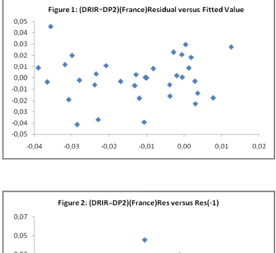
We used White test because of the fact that it is not sensitive to the normality assumption of the error terms. However, since it is a large sample test, we will use the F statistics of the auxiliary regression of the test with no cross terms (as it is argued in the literature that when it is performed with the cross terms it can be also regarded as specification test). When we look at Table 2, it can readily be seen that p-values for the null hypothesis stating that “There is no heteroskedasticity is present in data” are high enough for not rejecting the null. That is, we can conclude that there is no heteroskedasticity in the data. On the other hand it should be noted that for dependent variable DR and countries Japan and Australia, there is some form of heteroskedasticity as the corresponding p-values suggest significance at % 10 level. Nevertheless, as a remedy to the minor heteroskedasticity problems, the regression will be re-performed using Newey-West Heteroskedasticity and Autocorrelation Corrected Standard Errors. For illustration purposes, we plotted residuals that we obtained from the regression against the fitted values for France and the dependent variable DP2. As can be seen From the Figure 1, there is no observable specific pattern for the residuals.
26
In addition to heteroskedasticity, we also tested the existence of autocorrelation for the residuals. In order to do this, we performed Serial Correlation LM Test (with two lags). Since our sample size is not large for the individual countries, we took the F statistic for the auxiliary regression. The results are presented in Table 3. As the low p-values suggest, we generally reject the null hypothesis claiming that there is no serial correlation in the error terms. That is, for most of the individual countries autocorrelation exists. For illustration purposes, we provide Figure 2 showing the graph of residuals versus their first lags for France and the dependent variable DP2.
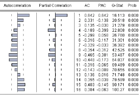
As a remedy for autocorrelation in the data, we added AR (1), AR (2) and MA (1) error schemes looking at the Correlograms for the residuals accompanied with West Heteroskedasticity and Autocorrelation Corrected Standard Errors. For the case of France and dependent variable DP2, the correlogram and AR (1) corrected residuals are depicted in the following Figures 3-4.
This pattern suggests that an AR (1) scheme for the error term. Having corrected for that scheme we obtained new residuals, and re-sketched the plot in Figure 2, which is shown in Figure 4. As it is seen in the Figure 4, the remaining errors are white noise.
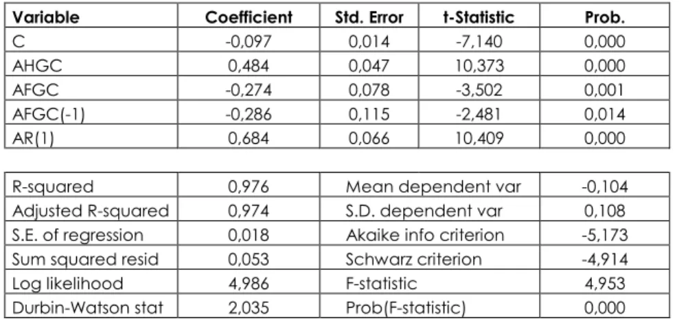
Having taken into account the cases of heteroskedasticity and serial correlation, we can now run the regressions for three different models with three different dependent variables. The model in Eq. (4) was re-estimated based on heteroskedasticity and serial correlation-corrected residuals. The estimation output is presented in Table 4-5-6.
27
In Table 4, the results of regressions for dependent variable DR are presented. It can be readily seen that the joint significance of the variables are high as the p-values for F-statistics are very low and R2 and adjusted R2 values are reasonably high. On the other hand, the significance of the coefficients for ACGH and ACGF are not generally high enough. For Canada and Portugal, both coefficients are significant at the %5 level; only the coefficient for ACGH is significant at the % 1 level for Japan and Norway, and significant at % 5 level for UK; only coefficient for ACGF is significant at % 10 levels for Italy. However, for dependent variable DR, the signs are not fitting to our prior expectations. (The sign checks will be examined below, while comparing the three models)
In Table 5, the results of regressions for dependent variable DP1 are presented. In this case, the joint significance of the variables is also high as the p-values for F-statistics are very low and R2 and adjusted R2 p-values are reasonably high. For dependent variable DP1, on the other hand, the for more countries significance of the coefficients for ACGH and ACGF are higher. On the other hand, coefficients for the first lag of ACGF are very significant for Australia, Canada, Japan, Norway, Portugal and Spain9. Nevertheless, for this proxy for the real interest rate, the signs are not seem to fit generally to our prior expectations according to our theoretical model.
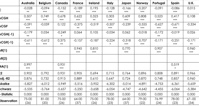
In Table 6 in previous page, the results of regressions for dependent variable DP2 is presented. The joint significance of the variables are also high as the p-values for F-statistics are very low and R2 and adjusted R2 values are reasonably high.
9
This observation is not fitting to our prior expectations, and it can be also observed for the dependent variable DR, DP2. This result will be discussed soon in the study.
28
Generally, the coefficients of ACGH and ACGF are very significant, and the signs are in line with what our theory suggests.
To compare the three models with dependent variables DR, DP1 and DP2 respectively, we cannot directly use their R2 and adjusted R2 values, since the dependent variables are different. Nevertheless, among the three competing proxies, DP1 and DP2 seems functioning well, in terms of high R2 and adjusted R2 values. The Akaike, Schwarz statistics seem to be nearly the same for all three equations. On the other hand when DP2 and DP1 are compared, it can be seen that DP2 creates more reasonable results that is parallel to our theory, in terms of significant coefficients for ACGH and ACGF and a reasonable scheme for the signs of coefficients. In Table 7, it can be seen that for dependent variable DP2, the signs for 10 of the 11 countries are reasonable.
Consequently, since the model with the dependent variable DP2 gives reasonable results, we decided to carry out the presence and the level of financial integration test based on the second proxy of real interest rate which is taking the growth rate of human capital into account.
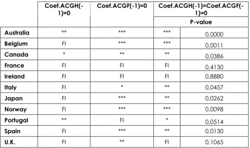
On the basis of our theory, if there is a presence of financial integration, then it should be the case that π3,π4 =0 andπ3=π4 =0; that is past lags of adjusted real consumption growth of rate for domestic and foreign country should not have an explanatory power on the real interest rate differential (proxy). In Table 8, π3 is
significant for Belgium, France, Ireland, Italy, Japan, Norway, Spain, and UK; π4 is
not significant for France, Ireland and Portugal; π3and π4 are not jointly significant
29
of both coefficients is because of the high significance of π4, which we think that it
is due to the fact that we compare the countries with US whose consumption growth rate and real interest rates are very influential on the world equilibrium level and, therefore, taken as reference anchor for determining the future consumption growth and the real interest rate. This problem can be solved by looking at the second lags of the ACGH and ACGF; however, as mentioned before this causes a decrease in degrees of freedom. ε π π π π π + + + − + − +
= 0 1ACGHt 2ACGFt 3ACGHt 1 4ACGFt 1 t
DRIR (4)
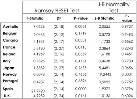
At this stage, in Table 9, we also present the results for Ramsey RESET test for the specification error and J-B Normality test so as to examine a possible specification error in our model. This is because of the fact that if our model has been incorrectly specified then we cannot draw reliable conclusion about the presence and level of financial integration.
As the table suggests, the p-values in Ramsey Test for the null (There is no specification error) are very low for Australia, Canada, France, Ireland, Spain and UK therefore we can reject the null and conclude that there is some sort of specification error in our model. On the other hand, the J-B normality test results suggest that the residual a follow a normal distribution for all countries except Norway. Therefore, the results of these two tests seem to contradict each other. We think that this results from the fact that degrees of freedoms for individual countries are not high enough to provide reliable output. To avoid the inconvenience and also develop an approach to understand the level of financial integration as well as presence we will utilize panel data in the next sub-section.
30
5.2 Panel Data Results
We will begin this section by first estimating the equation (3) for the strictly balanced data between 1981 and 1999 for 11 OECD countries. In the regression we include the two time lags for ACGH and ACGF as:
ε π π π π π π π + − + − + − + − + + + = ) 2 ( 6 ) 2 ( 5 ) 1 ( 4 ) 1 ( 3 2 1 0 t i ACGF t i ACGH t i ACGF t i ACGH it ACGF it ACGH it DRIR
This creates 209 observations for testing the financial Integration. We will assume that there is a fixed effect for the cross sections and random effects for the time period. We will use White cross section method for coefficient of covariance method. The results of the regression are shown in Table 10 for all dependent variables: DR, DP1 and DP2. As it is seen from the table, for the dependent variable DP2, the estimates are more reliable in terms of their significance and the expected signs. Therefore, we think that using the regression with dependent variable DP2 can create more reasonable results for detecting the presence. For the regression with DP2 that includes the growth rate of human capital stock in its nature as a dependent variable, the effect of the first lag of ACGF on the real interest parity differential is significant, which was also the case for the individual time series data. Since the reference effect of this variable, since it might be is taken as the anchor for the future consumption growth and real interest rate, we exclude it from our final financial integration test based on the Wald test. Therefore, we finally test the presence of financial integration for 11 OECD countries by testing whetherπ3 =π5 =π6 =0or not. For the corresponding Wald test the p value for π3 =π5 =π6 =0is 0.7613, which suggests that the null is true, implying that there is an evidence for the financial integration for the countries in question. To obtain the cross section affects on the
31
real interest rate parity (proxy) differential, namely the level of financial integration of the countries in the study, we ran the following regression:
ε π
π π
π + + + − +
= i0 i1ACGHit i2ACGFit i4ACGFi(t 1) it
DRIR (5)
The regression results are depicted in Table 11. As it is seen from the output, the coefficients for the regressors are highly significant at the % 1 significance level, which supports our theory. Moreover, it adds an additional factor (ACGFt-1) to our original theory by implying that the first lag of adjusted consumption growth rate for the foreign country might be taken as an anchor for future consumption decisions.
Finally, to interpret the results in Table 11, if the present adjusted growth rate of consumption in domestic country increases by 10 %, holding other factors constant, then the real interest rate differential increases by approximately 0.05 on average. This result makes sense since an increase in the present consumption growth rate means, loosely speaking, a decrease in the saving rate for the economy. Therefore, the capital accumulation will decrease, resulting in a lower capital-labor ratio, which makes marginal productivity of capital (the real interest rate) larger. All these mechanisms lead to a higher differential in the real interest rate of domestic and foreign country (holding the real interest rate of the foreign country constant). By the same reasoning, an increase in the present growth rate of consumption for the foreign country will have a decreasing effect on the real interest rate differential. If the foreign country has an economy that has an anchor effect for the other economies (U.S. in our case), then not only its present consumption growth rate but also its first lag will affect the real interest rate differential of the domestic country.
32
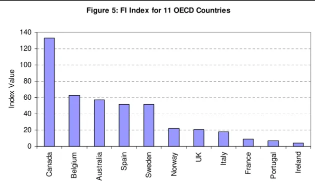
Finally, obtaining the cross sectional fixed effects, that is country specific effects on the real interest rate differential, we tried to develop a Financial Integration Index that captures the level of financial integration for the sample besides the evidence for financial integration. The index is calculated as:
1 _
_ _
_Index= Cross Section Fixed Effect−
FI (6)
According to this index, presented in Figure 5, Canada seems to be the most financially integrated country to the world (US), while Ireland seems to be the least. As to France, since this country is famous for the high capital controls in the past, the low level of financial integration, relative to other countries in the sample, seems to be captured by our index.
33
CHAPTER VI
CONCLUSION
In this study, after giving a brief review of the financial integration literature, an extension of the Euler test by Lemmen and Eijffinger (1998) was developed where new proxies for interest rate differentials were used in order to overcome the difficulty of measuring the ex post real interest rates, which may contain monetary shocks, and has considerable measuring variability because of the fact that reference nominal interest rates and the baskets for measuring the price changes are not equivalent across countries. In one of the proxies we used besides ex post real interest rate, we employed a transformation to capture the human capital growth rate effect on the real interest rates. Having looked at the results of the regressions with the dependent variables of the ex post real interest rate and the new proxies, we may conclude that the real interest rate proxy including the human capital growth rate factor functions well and creates reasonable results for the coefficients in our regression. In addition to our limited evidence for the financial integration in the time series data because of the degrees of freedom problems, we found strong results for the presence of financial integration for the sample of 11 OECD countries in the panel data setup. Furthermore, to determine the level of financial integration, we developed an index utilizing the country specific fixed effects on real interest rate
34
differentials. According to the index, Canada seems to be the most financially integrated country whereas Ireland is the least integrated in our sample.
To conclude, in this empirical study, we found strong evidence supporting our extended theory of Euler test. On the other hand, the results enhance this theory by implying that the big economies such as US can be an anchor for consumption decisions and real interest rate differential expectations. The future research on this topic might be on theoretical models that capture this stylized fact, which is supported by this paper.
35
SELECT BIBLIOGRAPHY
Balassa, Bela. 1962. The theory of Economic integration. London: George Allen & Unwin
Bayoumi, Tamim. 1990. Saving-Investment Correlations: Immobile Capital,
Government Policy, or Endogenous Behavior? IMF Staff Papers, June 1990, 37, 360-87.
Bayoumi, Tamim and Ronald MacDonald. 1995. Consumption, Income, and
International Capital Market Integration. International Monetary Fund Staff Papers, 42 (3), September, 552-76
Cline, William R. 1995. International Debt Re-examined. Washington, D.C.:
Institute for International Economics.
Feldman, Ricardo A. 1986. Japanese Financial Markets, Deficits, Dilemmas, and
Deregulation. Cambridge, MA: The MIT Press.
Feldstein, Martin, and Horioka, Charles. 1980. Domestic Saving and International
Capital Flows. Economic Journal, June 1980, 90, 314-29.
Feldstein, Martin. 1983. Domestic Saving and International Capital Movements in
the Long Run and the Short Run. European Economic Review, March/April
1983, 21, 139-51.
Fieleke, Norman. 1982. National Saving and International Investment. Saving and
Government Policy, conference Series No.2, Boston: Federal Reserve Bank of Boston, 1982 pp. 138-57
36
Frankel, Jeffrey. 1991. Quantifying International Capital Mobility in the 1990s. D.
Bernheim and J. Shoven eds. National Saving and Economic Performance, Chicago: University of Chicago Press, 1991, pp. 227-60.
Frankel, Jeffrey. 1992. Measuring International Capital Mobility: A Review.
American Economic Review, 82 (2), May, 197-202, 1992
French, Kenneth and James Poterba. 1991. Investor Diversification and International
Equity Markets. American Economic Review: Papers and Proceedings 81, 222-226.
Gartner, Lawrence M. 1993. Macroeconomics under Flexible exchange rate. New
York: Harvester Wheatsheaf.
George M. von Furstenberg. 1998. From Worldwide Capital Mobility to
International Financial Integration: A Review Essay. Open Economies Review, 9(1), January, 53-84, 1998
Hausmann, R. and L. Rojas-Suarez. 1996. Banking Crises in Latin America.
Washington, D.C.: Inter-American Development Bank.
Kaminsky, G.L. and C.M. Reinhart. 1996. The Twin Crises: The Causes of Banking
and Balance of Payments Problems. International Finance Discussion Paper No. 544. Washington, D.C.: Board of Governors of the Federal Reserve System.
Levine, Ross. 1996. Foreign Banks, Financial Development and Economic Growth,
in International Financial Markets. Claude E. Barfield, American Enterprise
Institute Press (Washington D C: 1996).
Milesi-Feretti, Gian Maria. 1998. Why Capital Controls? Theory and Evidence.
Sylvester Eijffinger and Harry Huizinga (eds), Positive Political Economy: Theory and Evidence, Chapter 8, Cambridge: Cambridge University Press, 217-47
Murphy, Robert. 1984. Capital Mobility and the Relationship between Saving and
Investment in OECD Countries. Journal of International Money and Finance, December 1984, 3, 327-42.
Obstfeld, Maurice. 1984. Risk Taking, Global Diversification, and Growth.
37
Obstfeld, Maurice. 1986. Capital Mobility in the World Economy: Theory and
Measurement, in Karl Brunner and Allan H. Meltzer (eds), The National Bureau Method, International Capital Mobility and Other Essays, Carnegie- Rochester Conference Series on Public Policy, Volume 24, Amsterdam: North-
Holland, 55-103
Obstfeld, Maurice. 1989. How Integrated Are World Capital Markets? Some New
Tests. G. Calvo, R. Findlay, and J. de Macedo, eds., Debt, Stabilization and Development, Oxford: Blackwell, 1989, pp. 134-55.
Obstfeld, Maurice. 1998. The Global Capital Market: Benefactoror Menace? Journal
of Economic Perspectives 1, 2 (Fall 1998), 9 -30.
Ortega, Daniel. 2006. Are capital shares higher in poor countries? Evidence from
Industrial Surveys. Wesleyan Economics Working Papers with number 2006- 023.
Summers, Lawrence. 1988. Tax Policy and International Competitiveness. Jacob
Frenkel, ed., International Aspects of Fiscal Policies, Chicago: University of Chicago Press, 1988, pp. 349-75.
Summers, R. And A.Heston. 1991. The Penn World Table: An Expanded Set of
International Comparisons, 1950-1988. Quarterly Journal of economics, 106 (May), 327-68
Sylvester C.W. Eijffinger and Jan J.G. Lemmen. 2003. International Financial
Integration, Volume I-II, Edward Elgar Publishing Ltd.
Sylvester C.W. Eijffinger and Jan J.G. 1998. Financial Integration in Europe:
Evidence from Euler Tests. Jan Lemmen (ed.), Integrating Financial Markets in
the European Union, Chapter 4, Cheltenha, UK and Northhampton, MA: Edward Elgar, 109-30, references
Tesar, Linda and Ingrid Werner. 1995. Home Bias and High Turnover. Journal of
International Money and Finance 14, 467-92.
Tobin, James. 1983. Comment. European Economic Review, March/April 1983, 21,
38
Williamson, John, and Molly Mahar. 1998. A Survey of Financial Liberalization,
Essay in International Finance. No. 21 1, Princeton University (November 1998).