Quantum polarization properties of radiation

г & і » ¥ - г г ш · г.'·-:

- « с • ¿ / S 3

QUANTUM POLARIZATION PROPERTIES OF

RADIATION

A THESIS

SUBMITTED TO THE DEPARTMENT OF PHYSICS AND THE INSTITUTE OF ENGINEERING AND SCIENCES

OF BILKENT UNIVERSITY

IN PARTIAL FULFILLMENT OF THE REQUIREMENTS FOR THE DEGREE OF

MASTER OF SCIENCE

By

Mithat UNSAL

August, 1999

‘АС.

-ΑΨ5- ■ U5S ІЭЭЭ

I certify that I have read this thesis and that in my opinion it is fully adequate, in scope and in quality, as a thesis for the degree of Master of Science.

Prof. Dr. Alexander Shumovsky(Pfincipal Advisor)

I certify that I have read this thesis and that in my opinion it is fully adequate, in scope and in quality, as a thesis for the degree of Master of Science.

Prof. Dr. Mefharet Kocatepe

I certify that I have read this thesis and that in my opinion it is fully adequate, in scope and in quality, as a thesis for the degree of Master of Science.

Prof. Dr. Vladimir Mirnov

Approved for the Institute of Engineering and Sciences:

Prof Dr. Mehmet B a r a y / /

Director of Institute of Engineering and Sciences

ABSTRACT

QUANTUM POLARIZATION PROPERTIES OF

RADIATION

Mithat UNSAL

M. S. in Physics

Advisor: Prof. Dr. Alexander Shumovsky

August, 1999

New bosonic operators, describing the polarization properties of photons at any point with respect to a source, are introduced. It is shown that, unlike the classical picture, the local quantum description of polarization needs nine independent local Stokes operators, forming a representation of the SU(3) sub­ algebra in the Weyl-Heisenberg algebra of photons. The Cartan algebra of this SU(3) determines the cosine and sine of radiation phase operators. It is shown that the use of plane wave photons can lead to wrong results for quantum fluctuation of polarization even in the far zone.

Dual representation of multipole photons is proposed. The exponential operator is diagonal in this representation, hence dual number states describe radiation phase states.. The discrete spectrum of exponential operator is found for dipole and quadrupole photons and a natural behaviour in the classical limit. Application of the results to the near-field optics is discussed.

Keywords and Phrases: Polarization, dual representation quantum phase, quantum near field optics

ÖZET

ISINIMIN KUVANTUM POLARİZASYON

Ö

z e l l i k l e r i

Mithat UNSAL

Fizik Bölümü Yüksek Lisans

Danışman: Prof. Dr. Alexander Shumovsky

Ağustos, 1999

Fotonların bir kaynağa göre herhangi bir konumdaki polarizasyonlarını tanımlayan yeni bozon işlemcileri tanımlandı. Klasik tanımın aksine, kuvantum polarizasyonun tanımlanmasında dokuz tane yerel Stokes işlemcisine ihtiyaç olduğu gösterildi. Bu işlemciler fotonların Weyl-Heisenberg cebrinin SU(3) altcebrinin bir gösterimini oluşturur. SU(3) cebrinin Cartan cebri ışınımın fazının kosinüs ve sinüs işlemcilerini belirler. Fotonlar için düzlem dalgaların kullanılmasının polarizasyonun kuvantum dalgalanmalarında, kaynaktan uzak bölgelerde bile, yanliş sonuçlar verdiği gösterildi.

Çok kutuplu fotonlar için çifteş gösterim önerildi. Üstel işlemci bu gösterimde köşegen bir matris halini alır. Bu da gösterir ki çifteş sayı durumları ışınımın faz durumlarını belirler. Üstel işlemcinin iki-kutuplu ve dört-kutuplu fotonlar için ayrık izgesi bulundu ve klasik limitte beklenen sonuçlar alındı. Sonuçların yakın bölge optiğine uygulanması tartışıldı.

Anahtar Kelimeler ve ifadeler: Polarizasyon, çifteş gösterim, kuvantum fazi, kuvantum yakın bölge optiği

ACKNOWLEDGMENTS

I would like to express my gratitudes to Prof. A. Shumovsky for his supervision throughout this work.

Very special thanks to Dicle Ozi§ for her moral support, encouragement and technical aid.

I wish to express my thanks to Özgür Çakır, Altuğ Özpineci, Suat Ekinci- Umud Devrim Yedçın and Özgür Oktel for their friendship.

C ontents

1 Introduction X

1.1 Intuitive introduction to local quantum polarization... 3

1.2 Dual representation of multipole photons and quantum phase . . 3

2 Q uantum Theory o f Polarization 5 2.1 Quantization of Electromagnetic field In a Spherical Cavity . . . 5

2.2 Photon Operators for a given P o la riz a tio n ... 10

2.3 Stokes Operators and Param eters... 12

2.4 Near Field P ro p erties... 14

2.5 Local Stokes O p e rato rs... 16

2.6 Position-dependent quantum o p t ic s ... 18

2.7 Dipole Field Polarization in Local p ictu re... 20

3 Q uantum phase via Polarization 22 3.1 Introduction to Quantum P h a s e ... 22

3.2 Dual Representation of Atom-Field S y stem ... 23

3.2.1 Quantum Phase via Angular M om entum ... 23

3.2.2 Dual Representation of A to m s ... 25

3.2.3 Dual Representation of Photons . 27

3.3 Atom-Field Interactions in Dual representation 29 3.3.1 2 dipole atoms in a Spherical Cavity 30

3.4 Local Description of Quantum Phase 33

4 Conclusion 42

List o f Figures

2.1 The components of an E-type radiation in the near zone . . . . 9 2.2 Zones for a simple radiating s y s te m ... 18 2.3 A dipole a to m ... 20

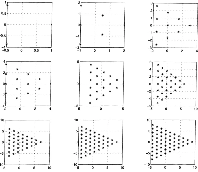
3.1 The discrete eigenvalue spectrum of non-normalized exponential operator in the complex plane is shown for dipole photons for n = l ,2 ,...,9 ... 38 3.2 As the number of photons goes to infinity, the eigenvalue spec­

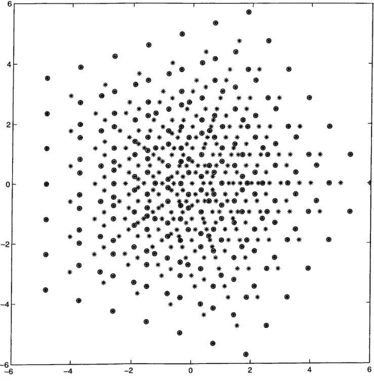
trum forms a two dimensional lattice in complex plane. Hence it covers the (0,27t) interval uniformly. 39

3.3 The discrete eigenvalue spectrum for quadrupole photons, ’o’ represents n = 6 case, while ’*’ represents n < 6 case. 40 3.4 The discrete eigenvalue spectrum for quadrupole photons. ’*’

represents n < 16 case. 41

C hapter 1

In trod u ction

Polarization discussions is an important part of physics for 300 years. C.Huygens, while working with calcite where he observed double refraction, discovered the phenomenon of polarization. He pointed out that:

”As there are two different refractions, I conceived also that there are two dif­ ferent emanations of the waves of light...”

During the same period. Sir I. Newton in his Opticks stated: ” Every Ray of Light has therefore two opposite Sides....”. [1]

In recent years, polarization measurement is an important tool for physical and optical measurements especially for quantum entanglement research. [2, 3, 4, 5] In spite of very important developments, the polarization is still treated from a classical point of view where the electromagnetic field is considered to be a totally transversal one. G.G.Stokes proposed the four Stokes parameter in order to describe the polarization state of the field. [6, 7] They are originally proposed from an operational point of view. The optical apparatus measures the intensity of the field hence the Stokes parameters are quadratic forms of field strength. This measurements determines the state of polarization of the plane wave.

But this formalism disregards the existence of longitudinal field. It is well- known that multipole radiation has both transversally and longitudinally po­ larized components. [6, 8] Actually, standard supposition in such analysis is to single out the generation of light by source and to look its spatial and tem­ poral evolution free of source efiects. This evolution or propagation region is

examined in three separate zones, namely near, intermediate and far zones of radiation, [6] since light exhibit remarkably different behaviors in them. Criti­ cal parameter in classifying the zones is the wavelength of the radiation. Only in the case of monochromatic light, a well-separated classification is possible. Another parameter is the dimension of the source, and for modern optical applications, typical light sources have dimensions much smaller than any dis­ tance of interest. This brings the concept of localized sources with additional assumption that it defines a closed system of charges and currents. Under these physical assumptions, light propagation from localized sources, in the frame­ work of classical electrodynamics, is described in terms of multipole expansion.

Usually, the optical measurement takes place in the far (radiation) zone where the longitudinal component of the field vanish and spherical waves are considered to be plane waves. But currently there are several advances in mod­ ern communication and computation technologies as well as developments of near field optical devices, like optical scanning near field microscopes (NSOM). As discrete degrees of freedom, polarization states of light considered to be a good basis for information coding. However, since polarization of light is a local property and information exchanges between quantum chips can occur in distances much smaller or comparable to wavelength, near field effects be­ comes important. Also, in near field light polarization also have a longitudinal component which can bring a new key to logical basis of |0l >, |1l >· Fur­ thermore, some of the information on the source parameters is trapped by the local, quasi-static mode around the source in the near-zone and not all the information can reach to the far zone.

For these purposes, it is necessary to know how the polarization behaves in the quantum domain where it is determined to be a given spin state of the photons [9] and investigate its spatial evolution. It is well-known that the radial component of the field exist in the near zone and decays as the separation between source and observation point increases. In the standard picture, the polarization is defined as transversal anisotropy of the field. But in order to take into consideration the near and intermediate field effects, spatial anisotropy should be considered rather than the transversal one.

1.1

In tu itiv e in tro d u ctio n to local q u an tu m

p o la riza tio n

From the classical definition of Stokes parameters, it is possible to obtain the quantum mechanical Stokes operator using the method of second quantization, [11, 16] namely. So, S i , S

2

, S

3

. These operators form a SU{

2

) subalgebra in the Weyl-Heisenberg algebra of plane photons. Since [5'i,5'2] / 0,the physical quantities described by these two operators cannot be measured at once. In quantum domain, the classical picture seems to be violated. In classical picture, we have phase information but not in quantum picture. For this reson, it is necessary to construct the complete set of quantum Stokes operators, then extend it to a local picture.

The quantum entanglement research based on cavity QED uses the polar­ ization state of a photon to store information. But plane wave description is irrelevant in this case since a source emits spherical photon with longitudinal and transversal polarization. The atoms in this picture are used as an inter­ mediary that causes one photon to interact with another. For these purposes, it is necessary to know how the polarization behaves in the quantum domain where it is determined to be a given spin state of the field.

By introducing local effective creation and annihilation operators describing the photons with given polarization at a given position with respect to a source, near and intermediate field optics can be constructed. Another essential point is that usage of plane wave photons will lead to wrong results in the quantum fluctuations of polarization even in the far zone. [10]

1.2

D u a l rep resen ta tio n o f m u ltip o le p h o to n s

and q u an tu m phase

Dual representation for both atoms and photons have been introduced in a very natural way. The main idea is to consider the radiation of a given quantum source rather then the free electromagnetic field. [12] Even in classical picture, the multipole radiation can be determined completely, in principle, if the source functions, namely current and charge densities, are known completely. With in

the quantum picture, the source dependence of the radiation can be considered in the following way. Since the total angular momentum / + M of the atom- field system is conserved in the process of generation, we can first construct the polar decomposition of J in the 2j -f 1 dimensional atomic Hilbert space Ha

according to the method by Vourdas. [13]Then for the phase dependent dual representation of the atomic SU(2) algebra, the radiation counterpart is deter­ mined which consist of the operators complementary to the atomic operators with respect to the constants of the motion. As a result, the phase states de­ scribing the dual representation for atoms and photons have been introduced. The phase number states and coherent states have been examined and com­ parison is made with the conventional states. A model Hamiltonian describing the behaviour of two atoms in a spherical cavity has been investigated in both conventional and dual representation.

There has been works on the determination of quantum phase in terms of polarization. [16] The polarization has been described in [16] by conventional Stokes operators and quantum phase variable is defined in the spirit of Pegg- Barnett approach [14, 15]which deals only with transversal polarization and so on.

One of the most important approach to quantum phase is operational ap­ proach which deals with what can be measured experimentally. [17] The oper­ ational approach is complementary to source-based approach which deals with what can be generated by a quantum source. [12] Notice that generation and detection process are quite related in the sense that they consider what can be transm itted from a quantum mechanical system to photons and vice versa.

Then a local description of quantum phase via local quantum polarization has been introduced. The eigenstates of the radiation phase are determined. The quantum phase has a discrete spectrum and a natural behaviour in the classical limit.

C hapter 2

Q uantum T heory o f

Polarization

2.1

Q u an tization o f E lectro m a g n etic field In

a Spherical C avity

Photons, quantum of electromagnetic field, can be described by states with well defined energy ftw, angular momentum, z-component of angular momentum and parity. [18]These photons are emitted and absorbed by the transitions in the systems with well defined values of the angular momentum and parity. The physical example to these systems are atoms, molecules, nuclei, quantum dots where the interaction is a function of separation between the particle, i.e when a rotation is applied to the whole system, the interaction energy remains invariant.

Let us consider a quantum source located at the origin of a coordinate system. The radiation is of 2 type with respect to its parity, namely electric (E) and magnetic (M) type. In case of (E) type radiation, the magnetic induction is transversal to direction of propagation, but electric field has a longitudinal (radial) component. And vice versa for (M) type radiation, i.e. the electric field is perpendicular to direction of propagation and magnetic field has a longitudinal component. Hence instead of working with electric and magnetic field, we can work with a single object, the vector potential A{f,t).

It is possible to construct the quantization of electromagnetic field in a spherical cavity with perfectly conducting walls by expanding the vector poten­ tial as a superposition of states with well defined values of angular momentum and parity. After expanding the vector potential in terms of vector eigenmode functions, it is possible to use method of second quantization [8, ll]to make a change to occupation number representation. At this point we can construct the physical observables of the field in terms of photon creation and annihila­ tion operators. In this construction, it is first necessary to fix the gauge of the field. In optics, the Coulomb gauge is generally used. (VA = 0). The vector potential of electromagnetic field in volume V, can be written in the form of an expansion:

Z ) [ax{Qjm)Ax{Qjm) + al{Qjm)Al{Qjm)]

Q j m X

(2.1)

where A = M, E determines the type of radiation. The vector potential for magnetic 2‘^-pole radiation is

Am =

\ VujQ r (2.2)

and the potential for electric 2‘^-pole radiation is

Aß = 2Trhc^

{2j -f l)Vu)Q

—t

(2.3) where fj{Qr) is a function proportional to linear combinations of spherical Hankel function of first and second type, depending on boundary conditions. The spherical Hankel function can be expressed as

= ji{p) + ^Mp) f^?\p) = f^?\p)* = ji(p) - ^Mp) (2-4) where j;(p), n/(p) are spherical Bessel and Neumann functions. All of the spher­ ical Neumann functions are singular at the origin but not spherical Bessel func­ tions. That means in the free field expansion, only ji{p) will appear since it has no singularity. But when it is necessary to consider the source, n/(p) will appear naturally since the field due to a source has a singularity at the space point where the source is located. But at this point, it is necessary to keep in

mind that a source has an spatial extension. The explicit form of the first few Spherical Hankel functions are the following.

= -o^P

V

Pj

ip h ÿ \ p ) = leip i + ^ - 4 ' 1 + ^ -. P P P |2 P } 1^ ' The normalization condition is the following;

I fj{Qr)fj{Q'r)r'^dr = V

6

qq>

Jo

(2.5)

(

2

.

6

)

and Q is the wave number, with dimension reciprocal to the length which for each J goes through a set of discrete values determined by the condition fj{Qr) = 0 In magnetic type radiation, the electric field strength and magnetic induction are equal to

E u i Q j m ) - iQAMiQjm) BM{Qjm) = V x AM{Qjm) (2.7) The electric field strength in an electromagnetic field corresponding to mag­ netic multipole radiation is thus always transversal to the radius vector, in the direction of which the wave propagates. = 0

In electric type radiation, the electric field strength and magnetic induction are equal to

ÊEi Qj m) = iQÂEiQjm) BEiQjm) = V x AE{Qjm) (2.8) The magnetic induction in an electromagnetic field corresponding to electric multipole radiation is thus always transversal to the radius vector, in the di­ rection of which the wave propagates. (Be-E) = 0

Before the transition to the quantum description, it is necessary to investi­ gate the properties of spherical vector harmonics. Let the spin operator and orbital angular momentum operator be denoted by S and L. then the operator of total angular momentum is

J = L + S (2.9)

The eigenfunctions YjLm of the operators and is called the spherical vector harmonics and satisfy the following equations:

= .j(j + l)Y.JLm

The components of the spin operator of a particle with i? = 1 can be written in the form of well known 3 x 3 matrices, Sx, Sy, Sz which satisfy the usual commutation relations of an angular momentum. The spin wavefunctions Xiy, satisfy the following eigenvalue equations.

S Xifi — SzXi/j. — fJ'Xi/j.

The spin wave function Xi,i, Xi,o, Xi,-i are given by the vectors

(2.11)

1 >1 0 ^ / o \

0 1 7 0

U J l o j 1 /

(

2

.

12

)

Since orbital angular momentum and spin operator commute, one can use the rules of the vector addition of angular momenta to form the vector spherical harmonics from linear combinations of the spin functions xi^ and spherical

harmonics Thus we have

Y j L m — ^ I L n T T l f l \ j T 7l > X\fiY^L,Tn—n { P i 4'') (2.13)

where < I L n m — ^i\Jm > are the vector addition (Clebsh-Gordon) coefficients. The coefficients vanishes if the following conditions are not satisfied.

J = L + 1 , T , |T - 1 |; m = ± J , ± ( J - l ) , (2.14)

Under an inversion, spin wave function xi^ change sign, but the spherical harmonic is multiplied by (-1 )^ . Thus the spherical vector har­ monics correspond to a state of well defined parity which is equal to ( —1)^···^

The YjLm form an orthonormal complete set.

/

YjLmYj'L'rn'd^ — ^JJ'^LL'^n (2.15)

Three spherical vector function belong to each value of J which differ ac­ cording to their L values. The parity of Yjjm is equal to (—l)'^''·^ while the parities of Yjj+im and Yjj-im are (—l ) “^·

The spherical vector function Yjjm is at right angle to the propagation —t

direction n = QIQ and is usually called transverse magnetic spherical vector function and is denoted by the notation

^

^Jm — ^JJm (2.16)

Figure 2.1: The components of an E-type radiation in the near zone

Let us now consider a second spherical vector function which is perpendic­ ular to both Yj!^ and propagation direction n. It can be constructed by the following way.

Y i , = - i ( n X ? " ) (2.17) defines a photon state with angular momentum J and parity (—1)·^. This function is called electrical transverse spherical vector function. It is linear combination of two spherical vector functions, corresponding to orbital angular momenta J -f 1 and J — 1 in the following way.

_

^Jm —

1

V2J T I [VjYjJ+lm + y/J + IF /J-lr (2.18) In states described by electrical vector spherical functions, the orbital angular momentum of photon does not have a well defined value. We therefore can not split the total orbital angular momentum into a spin and orbital part.

It is possible to form one more vector function, namely longitudinal spher­ ical vector harmonics, directed along the propagation vector. It has a simple form

YL· = ñYj„(ñ) (2.19)

Notice that these three vector functions, Yjm^Yjm·’ Yfm are mutually orthogonal for different values of J and m, for the same values of J and m, they are mutually perpendicular for each value of propagation direction.

10

Now, let us consider the second quantization of the classical electromagnetic field in a spherical cavity. The transition to quantum description in the occu­ pation number representation corresponds to replacing the field amplitudes by the operators satisfying bosonic commutation relations.

[a\{Qjm),a\,{Q'j'm')\ = Sxx,

8

QQ,

8

jj,

8

mm'· where all other commutators are zero. After substitution

(2.20) (2.21) transform to H = UujQ[a\{Qjm)ax{Qjm) - | - h Q J m X

(

2

.

22

)

and the vector potential (2.1) becomes an operator of the following form.

A = ^ \ax{Qjm)Ax{Qjm) + a l ( Q j m ) A l { Q j m ) (2.23)

n \ L J

Q j m \

Both the electric field E = \ ^ A and and magnetic field (2.7,2.8).B = V x A are operators after second quantization.

The operator <i\{Qjrn)a\[QjTn) corresponds to number of photons cor­ responding to multipole radiation. Each photon in the state XQjm has a wavenumber Q, square of angular momentum 7(7 -|- 1)^^, z-component of an­ gular momentum mh and parity (—1)'^·'·^ ioi X = M and (—1)*^ for A = jE

2.2

P h o to n O perators for a given P olariza­

tio n

The spatial properties of a monochromatic pure multipole radiation (at a given J) of a quantum source, either magnetic or electric type 2·^ pole radiation, can be described by a vector potential operator (2.23). Let us replace the quantum source at the origin, then the system has a rotational symmetry. Since [J, H] = 0; the most convenient quantum representation of the problem is provided by the photons with definite angular momentum and parity which

11

are the so-called spherical photons [8]. In this case, a monochromatic photon with total angular momentum can be characterized by

2

j + l quantum numbers. In this representation,, the photon operators are a\jm{k), (/::). Each photon in state a\jm{k) has wavenumber k, angular m o m e n t u m a n d parity (—1)·^·*·^ (for M-type) and (—1)·^ (for E-type). Since we will restrict our quantum source to a definite one, we will denote a\jm{k) = ajm- The bosonic commutation relations are satisfied for

(2.24) The total angular momentum of a photon is J = S + L where S is spin operator

—^ ^

and L is orbital angular momentum operator. At a given J value, we can make the following expansion for positive frequency part of vector potential A.

= E

Xm

E

/JL·= — l m = —j

jm (2.25)

Here Xfj, are photon spin wavefunctions and satisfy orthonormality condition.

xi-XM (2.26)

are well-known functions composed of fj{kr) which is a linear combi­ nation of Hankel functions of first and second kind where the coefficients are determined with respect to boundary conditions, Yim{^i

4

’) spherical harmonics and Clebsch-Gordan coefficients. It can be both magnetic and electric type.

fj{kr) < IjixTn - ii\jm > Yjm.{0, <f>) M-type j+ifj+i{kr) < Ij + Ifrni - f i \ j m > Yj+irn-^

0

, <f>)

- f j - i { k r ) < Ij - lfj.m - filjm > Yj-im-ti{0, (f>) E-type (2.27) l

2

‘whc

~ w

Any component of A{f) can be written as

’jm (2.28)

m = - j

Let us now consider the commutator of /l/i(r) and Aj^,(f) at the same space point. It is

aU?)] = E V,„(r)v;,„(f) s V„,(r1 (2.29)

m.=—j

where V^^/(r) is a position dependent (3 x 3) Hermitian Matrix. There exist a local unitary transformation U{f) for each space point r which diagonalize the matrix V(f)

12 /7 ( ^ í/t( f ) = 1 t/t( f ) V ( r ) t/( ^ = W{r) = w+ 0 0 0 Wo 0 0 0 W-(2.30)

The diagonal elements of W matrix are real and positive. At this point, we can define an effective operator

I

-1 j a^{f) = 1 ,t E E v M ñ »j m (2.31) m = —j

The commutator of a^(f) and al(f) at the same space point yields bosonic commutation relations.

.t

Vr [a,,(r),a^.(r)| = 0 (2.32)

The second relation follows from the linearity of a^(r) with respect to ajm- a^(f) and a\{r) can be interpreted as annihilation and creation operators of polarization of a field at a given point. These operators form a representation of Weyl-Heisenberg algebra of photons at any point r in three dimensional space. Note that the orbital part of angular momentum of photons cannot be well defined in the states with given polarization. That is due to the fact that the photon is a zero mass particle.

In order to understand the meaning of these operators, let us express the expression for the Hamiltonian in terms of these operators.

fi m

.t/

(2.33) where IT'^(r) stands as an weight factor in front of a/i(f)a^(f) hence forming the intensity operator Ifi{r).

2.3

Stokes O p erators and P aram eters

Polarization, in the conventional sense, is the measure of spatial anisotropy of the field in the plane perpendicular to the direction of the propagation

13

of the radiation. [19] This follows directly from the transversal solution of homogeneous wave equation.

1 d^A

VM

dt^

0 (2.34)

In this solution, both the electric field E = \-§iA and and magnetic field B = V X y4 are perpendicular to each other and to the direction of propagation k. There is no rotational symmetry around the k axis hence the wave is polarized.

—^ ^

Both E and B can be used to specify the polarization but since both can be derived from vector potential, it is better to use A per se.

The vector potential at a given point in space can be written as Ao(t)e~'‘^* where .Ao(<) is a complex amplitude and very slowly changing function of time. For monochromatic light Ao is a constant and determines the polarization.

Experimentally, the polarization properties of radiation is investigated by passing it through some optical devices and measuring the intensity at some detectors. This means the time averages of the quadratic form of field am­ plitude is measured. Hence the polarization properties must be described by some quadratic functions of the field.

Because of averaging process with respect to time, the fast oscillating parts and Aq^Aq^c'^'^^ vanishes. The polarization properties of light is

characterized by the second rank Hermitian tensor [19]

aP (2.35)

Because of transversality of Aq the index a and ¡3 can only take values I and 2. The trace of the polarization tensor,/"«« is the energy intensity of the field. Because of hermiticity condition P

\2

= / 2*1· That means three real number is needed in order to describe this tensor, which form the conventional set of Stokes parameters.

The definitions of Stokes parameters in terms of the circular polarization basis:[7, 6]

»0 = \ t l . E ? + K . E \ \ s, = 2A e|(£ ;.£ )'(el.£ ;)),

s , = 2Iml(il.E)'(i-_.E)],

14

Here e± Ξ (ei ± ie

2

)/y

/2

and (¿o)^ = (-si)^ + (·*2)^ + (·53)^· This relation origi­ nates from the fact that the four Stokes parameters are not independent, they depend only three quantities, the magnitude of the fields and relative phase among field components. The parameter sq above, measures the relative inten­

sity of the wave, the parameter S3 gives the preponderance of positive helicity over negative helicity, and the parameters Si and S2 give the phase information in terms of the cosine and sine of the phase difference between two circularly polarized components.

The quantum counterpart of Stokes parameters (2.36)in terms of circular polar­ ization basis is provided by conventional Stokes operators that can be obtained by standard quantization of free electromagnetic field in the representation of ’’plane photons” (the photons having given energy and linear momentum) as follows [11, 16]:

60 = ( α |α + -f α1α_), S\ = (α1α+ -h α |α _ ), 5

2

= — — α |α _ ),

53 = ( α | α + - α 1 ο _ ) . (2.37)

In this construction, a,,, and at are creation and annihilation operators for photons with given linear momentum and polarization σ. Apart from a factor of 2, the operators 5; (/ = 1, 2,3) form a representation of the SU(2) subalgebra in the Weyl-Heisenberg algebra of plane photons. Since [5 i , 52] Φ 0,the physical quantities described by these two operators cannot be measured at once. In view of the standard interpretation of the Stokes parameters (2.36), which are expected to be the averages of the operators (2.37), this means that the cosine and sine of the phase difference between two components with opposite helicities cannot be measured simultaneously. But this seems to be irrelevant from a physical point of view. Since two different functions of the same operator must necessarily commute.

2.4

N ea r F ield P ro p erties

Note that the above construction of Stokes operators do not take into account the existence of longitudinal (radial) component of the field. But it is well

15

known that radiation from a localized source, either classical or quantum, has radial component. The radial component vanishes in the far zone and exist in the generation zone and near zone.

The polarization properties of light is characterized by the second rank 3 x 3 Hermitian tensor [20]

Paß — AQoiA.(jß =■ (2.38)

Transversality is not required any more and the index a and ß can take values 1,2,3. The trace of the polarization t e n s o r , i s the energy intensity of the field. The conventional 2 x 2 polarization matrix (2.35) can be obtained by setting AoazzO - 0.

The nine elements of polarization matrix can be determined by 5 real pa­ rameter. These are three intensities and any 2 out of three phase difference. The five generalized Stokes parameters can be chosen as follows.

•So _ \ ^ TP* Jp m •Si = _{2 R e { E l E o + E * E _ + E*_ E * )} •S2 = 2 I m { E l E o + E * E . + e _{:- E + )} •S3 = E ^ E ^ E I E -S4 = E * ^ E + -1- E * _ E . - 2 E ; E o (2.39) The physical meaning of these parameters are the following, sq is the intensity

of the field, S3 gives the preponderance of positive helicity state over nega­ tive helicity state. S4 gives the preponderance of circular polarizations over longitudinal polarization. si and S2 give the phase information.

By second quantization method, one can obtain the following generalized Stokes operators from (2.39).

- . t . So = 772 .^1 = ^2 = 63 = a].a+ — a i a _t t ^4 = 0+0+ + 0- 0- — 2aoOoi t t . + a_a+ . In this construction.

15„S2] == 1 5 . , 5 o1 = ( 5 2 , 5 o) = 0

(2.40)

16

hence the physical quantities corresponding to these operators commute. That means, one can get phase information from this construction opposed to con­ ventional Stokes operators ( 2.37).

Note that these operators are the total set of independent bilinear forms above, is represented by the generators of SU(3) sub-algebra in the Weyl- Heisenberg algebra.

t t

a\.a^ — «0^0 — a_a_t t <tla_ a\.a^

\{a\aoa\a^) |(a|a_-f-alao) |(ala+-f-a|a_) (2.42)

- GoO-i-) ^ ( 4 « - ~ «-«o) ^ ( a l a + - a | a _ )

These operators are not totally independent. Eight of them are really inde­ pendent which is the number of generators of SU(3) algebra. But in addition, there is intensity operator which commutes with all the generators. One can see that the five generalized Stokes operators can be expressed in terms of lin­ ear combinations of generators of SU(3) algebra. Moreover, the operators S\ and S

2

form the Cartan algebra in SU(3). But the eight generators and one intensity of SU(3) contains much more information then (2.40).

Let us also denote that (2.42) can be considered as some representation of polarization matrix in quantum domain. Unlike the classical case, the elements of quantum polarization matrix are specified by nine independent Hermitian operators. Therefore, the number of independent Stokes operators must also be nine.

2.5

Local S tok es O perators

Let us consider know the polarization properties of the quantum multipole radiation for an arbitrary j , which is not necessarily one.(dipole case). Polar­ ization, the spatial anisotropy of the field, is a local property of the field. The polarization matrix is a local 3 x 3 Hermitian matrix. One can reconstruct the local polarization matrix in terms of effective creation and annihilation operators of polarization.

17

Note that the operators a |(r),a ^ /(f) are quite different from the _{' j m >} operators. The operators ajm describing the multipole photons are independent of position, they act in

2

j + 1 dimensional space which coincide with three dimensional space only in the case of dipole photons. are local operators acting in three dimensional space and takes into account the spatial properties as well as the quantum nature of multipole radiation at any distance from the source. These operators coincide with the dipole photons in the generation zone.

These operators can be used to construct the near and intermediate field zone quantum optics in addition to far zone quantum optics. One can write the local Stokes operators in this way, from the generators of the local SU(3) algebra in the Weyl-Heisenberg algebra of photons, describing the independent Hermitian bilinear forms in the creation and annihilation operators. The local Stokes operators are the following:

So(ri = s , i n = -i[£{r) - e \ i ) ] = a|(f)ii+ (f) - a l(r)a _ (r) ¿4(r) = a\{f^a+{f) + a t . { r ) a - { r ) -

2

al{f)ao{r) Sa{f) = a |(f ) a o ( ^ + H.c. = -i[a\.{r}ao{f) - II.c.] - al{î^a-(r) + H.c. S s i ^ = -i[al{r)a^{f) - H.C.] £{r) = a|(r)o o (r) + (2.44)

A careful investigation showed that there are nine Stokes operators. The ex­ pectation values of these operators over physical states will give the following information. So{r^ is the local intensity of the field. S\{r) and S

2

{ ^ are the claimants of phase information, relative phase angles, A+_, A^-o, Ao_ where

^

0,0

= argAc{f) - argAp{r). (2.45) . 5'3(f) gives the local preponderance of positive helicity over negative helicity and Si{r) the preponderance of circular polarization over longitudinal polar­ ization. 65(7^, SQ{f) and 67(7), Ss{f^ gives phase information about A+o and A_o respectively.

18

The commutator [¿'i(f), 5'2(^ ] = 0, so that the corresponding physical quantities can be measured at any point at once.

2.6

P o sitio n -d ep en d en t q uantu m o p tics

It is well-known that the fields from a localized source, has very different prop­ erties in the different zones. [6] Let us point out the limits of the zones. As implied in the introduction, a well separation is only possible in the case of monochromatic light since the wavelegth of radiation has a huge spectrum from 7 -rays (A ~ to radio frequency (A ~ 10®m). [1]. But for our purpose, let us assume that the source is localized to a very small region com­ pared to wavelegth. If the source size d < < A, then there are three distinct spatial regions. generation zone near zone intermediate zone far zone

Figure 2.2: Zones for a simple radiating system

• Near (static) zone d « r « X

• Intermediate (induction) zone d < < r ~ A • Far (radiation) zone d « X « r

The field has very different properties at different zones. In the near zone the fields have a character of static fields with radial components and its variation with distance depends on the detailed structure of the source. The near fields are quasi-stationary, oscillating harmonically as In the far zone, the vec­ tor potential behaves as an outgoing spherical wave with an angular dependent coefficient. The fields are transversal to radius vector and falls of as 1/r. Thus the field corresponds to radiation field. In the intermediate zone all power of r/A must be retained. Notice that for a localized source, the total charge of the source is independent of time since there is no out or in flux. Thus the

19

electric monopole part of the source is static. The fields with harmonic time dependence have no monopole terms. Hence a field with harmonic time dependence is created at least by a dipole. This classical argument is related with fact that the minimum total angular momentum of the photon is 1. Or in another word, the photon can be created by a transition with \j — j'\ > 1 which implies that the electromagnetic field is a vector field.

By using the local operators, the notions of quantum optics can be reinves­ tigated [20]. For example, the normalized variance of the photon distribution i.e. Mandel’s Q-parameter which gives the statistics of photons is a position dependent parameter now. Hence a local Mandel’s Q-parameter should be defined.

< [ÍS.a\{

7

^a^,{f)Y > - < al(f)a^{f) >

Ai

(2.46)

< a/i(f)a^(f) >

Even though the parameter is a local one, it gives a global property of the field, namely, its statistics. For example, for the coherent state, Qn{r^ = 0 everywhere which implies a Poissonian distribution for coherent state and a global property of the radiation field.

The coherent states [21], which is defined by the eigenvalue equation for the non-Hermitian annihilation operator, with respect to the operators of photon with given projection of angular momentum

|o; >—

(^)

>,

m = - j

is also a coherent state with respect to because of the linear relation between annihilation operators.

a^(r)|o! >=

>

Otfi(v) — OLwMiimiX^

m=—j

The position dependent coherence parameter is of the following form.

1 j

a,

n'^-lrn=-j

(2.47)

The local property of coherence parameter implies that even though the field has all three polarization in near and intermediate zone, it will reduce to two transversal polarization in the far zone.

20

2 .7

D ip o le F ield P olarization in Local p ictu r e

Let us consider that a dipole atom is located at the origin of the coordinate

i _ i m=+l m=0 m=-l

J—A, --- ---

---j ’=0.

Figure 2.3: A dipole atom

system. In the generation zone, one has fi = m. In the near and intermediate zone, fji = —1,0,1. But in the far zone, since V^-o,m vanishes, the intensity of longitudinally polarized component of the dipole radiation tends to zero. T hat means in the far zone, the radial component /x = 0 ic in the vacuum state. In this case, the expectation values of generalized Stokes operators are the followings: < 5 o ( f ) > = < > < ^2(r-) > < 5 3(r-) > < 64(r) > < Ssif^ > ß = ± l = 2Re < al(r)a+('r} > =

2

I m < a i(r)a + (r) > = < a |(r^ a + (r) > — < a l(r)a _ (f) > = < S o { f ) > = < S'6(r) > = < .Srif) > = < >— 0 (2.48)

which coincide with classical phase parameters determined in the circular po­ larization basis. Hence, the polarization of quantum dipole radiation at far zone looks like that of the plane wave photons.

But there is a very fundamental difference in the quantum fluctuations of generalized Stokes operators in the far zone and conventional Stokes operators. Let us consider variance of The fluctuations for conventional (2.37) one is

< (A5i)^ > = 2Re < (Aola^.)^ > -l-2(< < a |a _ > p)-f < > -|- < n_ > (2.49)

21

and for generalized (2.44) one but radial mode in vacuum is

< (A^i)^ > =

2

Re < (A aia+)^ > + 2(< n+n_ - | < a |a _ > |^) +

< > + < n_ > -\-2Re < a+a_ > + < n + > + < n _ > (2.50)

The underlined term arises even though the radial polarization is in vac­ uum, but nevertheless it exist and the additional three terms come from the commutation relations. The presence of these terms increases the the quan­ tum fluctuations of transversal polarization and changes them qualitatively since the term include 2Re < a\.a^ >, a phase dependence.

This result shows us that the use of plane waves of photons rather than the spherical waves of photon can lead to a wrong result even in the far zone. It is worse to use the plane waves of photons in the near and intermediate zone where the radial component of the field is no more in vacuum. Let us also note that the quantum fluctuations of polarization is very important in the quantum entanglement research since the existence of radial field, even in the vacuum state, increases the noise in the system.

C hapter 3

Q uantum phase via

P olarization

3.1

In tro d u ctio n to Q uantum P h a se

The problem of identifying an Hermitian phase operator that corresponds to the phase of a quantized electromagnetic field has been debated ever since Dirac’s first paper on the quantum theory of radiation [22]. One of the most popular and important method is the one by Pegg and Barnett [14], is based on the contraction of the infinite dimensional Hilbert space of photon states 'Hn- In this construction, quantum phase is determined in a finite dimensional subspace of l-Ln· After the calculation of the expectation values, the dimen­ sionality of this subspace is sent to infinity in order to cover the whole Hilbert space. But in this picture, because the change in the algebraic structure of photons, one get wrong results for quantum fluctuations.

One of the most important result is that obtained by Mandel et al [17]. They proposed operational approach to the quantum phase . The main idea here is to define the phase operator in terms of what can be measured in real experiment. This analysis leads to different phase operators for different measurement schemes, with the strong statement that, there is no unique phase variable, describing the measured phase properties of light.

One recent approach is the source — based approach by Shumovsky [10, 23, 24]. The main idea is to consider the radiation of a given quantum source

23

rather than free electromagnetic field. Actually, the experimental schemes of the phase measurement mostly rely on the photon counting experiments which include interaction of light with a macroscopic detecting device. In this case, it is assumed that light is prepared in some quantum state which is a result of some interaction. The generation of photons by an atom is the main one. Thus, it is natural to extend the operational approach and examining the phase problem in terms of what can be generated. Actually, the main philosophy is to consider “what can be generated in nature in any kind of process” and investigate the properties of this radiation.

Our aim is to develop this beautiful formalism to a local one. The reason is simple. [27] The field created by a source has different properties in the gen­ eration, near, intermediate and far zone. The local intrinsic phase properties of photon will be investigated.

Moreover, a new representation of photon operators describing pure mul­ tipole radiation will be discussed. This representation involves the azimuthal angle of the angular momentum of photons.

3.2

D u al R ep resen ta tio n o f A to m -F ield S y s­

tem

3.2.1 Q u an tu m P h a se v ia A ngular M o m en tu m

Consider a radiation of an atomic transition between two states with definite a.ngular momentum and parity. In such a case, the most convenient quan­ tum representation of the problem is provided by the photons with definite angular momentum and parity which are the so-called spherical photons. Let us specify the transition under consideration as an electric 2-^pole (£'^-^^-type) transition with the excited state { J = j ^ m — ±j , ± j — 1, ...0} and ground state { J' = 0,rn' = 0}. If we restrict our consideration by a single-mode case as in standard Jaynes-Cummings model [25], then the Hamiltonian in the rotating wave approximation takes the form

+ j

,

,

H = E

24

The Hamiltonian describes the bare two level atom, the field and interaction of the single mode field with the atom. The atomic operator

Rmm' — ll^)(^ II

(3.2)

is shorthand notation for the transition between between states \\jm > and >. g is a, coupling constant depending on the volume of the quantization cavity. The degeneration of excited state is 2j + 1.

The angular momentum of exited atomic system is described in SU(2) al­ gebra with generators

j Jz = m R mm m = —j i -1 m = - j j J - = ¿ \J(j + m){j - m + l)R„,+ir m = - j + l

which obey the standard commutation relations

(3.3)

(3.4)

(3.5) and one can construct the Casimir operator in the finite dimensional Hilbert space of atom.

f ' = = Y , Rmm = j ( j + 1 ) X U (3.6)

7n = - j

One can obtain the exponential operator by the polar decomposition of SU(2) algebra. [13]

Using J+ = Jr^A and EaE \ = 1, one gets

i- i

Ea = Y Rm+lm + R-₃₃ (3.7) m=-j

which is the exponential operator in terms of atomic operators. Two interesting properties of atomic exponential operator is the following. E '^ = 1, E^a '^^ = E

for any integer k.

Notice that phase properties of the atomic radiative transition can be de­ fined by the polar decomposition of the corresponding SU(2) algebra, describing

25

the angular momentum of transition. But, the polar decomposition of SU(2) algebra cannot be performed in the case of photons. [26] That is the Casimir operator of enveloping algebra cannot be uniquely determined in the whole Hilbert space corresponding to the photons.

The angular momentum M of the electric dipole radiation is represented by the following operators.

+1

ma+a,n m= —1

M+ = y/2(a^ao + a ^ a .)

M_ = V^(ao ti+ + aico) (3.8)

form an SU(2) algebra for photons in the Weyl-Heisenberg algebra. The total angular momentum of the system is J + M . Since[J + M , /f] = 0 , total angular momentum is a conserved quantity.

Even though the polar decomposition is not possible for photons, one can show that the exponential operator for photons can be written in the form for an arbitrary j

^ = Y + aijCij (3.9)

which complements the atomic exponential of the quantum phase operator. The sum Ea + is an integral of motion.

[Ea+ S , H ] = 0 (3.10)

which means the phase information in the system, at least in the azimuthal phase, is a conserved quantity. The phase information can be transmitted from the source to the field and vice versa.

3.2.2

D u a l R ep re sen ta tio n o f A to m s

The eigenvalue equation for the atomic exponential phase operator for an ar­ bitrary J is the following.

(3.11) where and ¡i = - j , - j + 1, ...j - l , j . This equation determine the dual with respect to atomic Hilbert space Ha- The states > are the ’’phase

26

states” of atomic system where the exponential operator is diagonal [13]. Phase states can be expressed as linear combination of angular momentum states, as a discrete Fourier Transformation,

1

(3.12)

m = - j

The inverse discrete Fourier transformation is 1

m > = (3.13)

The SU(2) algebra can be constructed in dual representation with the fol­ lowing generators.(The dual atomic operator

a:««, = ll$«){í„■|| (3.14)

denotes the transition between between states > and >)

= i -1 = ^ \/( i “ + /^ + /1=-J j f i = - j + l

which obey the standard commutation relations

l 4 * \ 4**1 = ± 4 * ’. [4**. 4*>] = 2j w .

(3.15)

(3.16) and one can construct the Casimir operator in the finite dimensional Hilbert space of atom.

(/♦ ))" = ¿ = ,{ j + 1) X 1 , (3.17)

The dual representation in terms of phase states gives the following diagonal form of Ea

27

3 .2 .3

D u a l R e p r e se n ta tio n o f P h o to n s

The exponential operator for photons can be written in the following form for an arbitrary j

E at,ara-i + aijGj (3.19)

m = - j+ l

This operator is not diagonal in the representation of spherical photons. But it can be diagonalized by using the following transformation.

(3.20)

(3.21) — ---- 1---- NP

The operators obey the canonical commutation relations.

[ A „ A A = D |/iI , 4 ) = o (3-22)

One can interpret these operators as the annihilation and creation operators of a given azimuthal phase angle.

Then the exponential operator of the photons becomes

(3.23)

where is the phase angle.

One can also observe that due to linearity of this transformation (3.20), the vacuum stability condition is satisfied, that means the action of the annihilation operators over the vacuum state is zero.

ajm\vac >= Ajfi,\vac > = 0 V/x,m (3.24) which implies that the vacuum of both operator has one and the same vacuum. Hence; one can define dual representation number states. These states are obtained by the action of creation operator a|^.

_a\ Yi‘

Wa > = {A]^y>^\vac > (3.25)

28

These dual number states are orthonormal and form an orthonormal com­ plete set in the Hilbert space dual to the conventional set of number states.

^Ul/'nn' y y \^H ^)l\ 1 (3.27) fl

The form of the number operator in both representation are

y~! ~ ^ (3.28)

^ m.

hence the transformation conserves the total number of photons.

Any phase state can be expressed in terms of conventional number states \nm >■ But the transformation is not simple one, even in the case of dipole photons, one gets the following relation.

{aIy>^ k+.i'o.»'- > =

n

= n h ^ E E

nii=0 - «+ - ^-)! Inif., — > (3.29) Let us also mention some properties of exponential operator. (3.23) is not Hermitian, but it commutes with the total number of photons. The dual number states are the eigenstates of the exponential operator.

(3.30)

The bosonic commutation relations of the operators implies that one can generate the coherent state oh the phase states by the action of dis­ placement operator on the vacuum.

(3.31) Let US define the direct product of coherent states for a fix j which is an

eigenstate of annihilation operators.

+j \rj> = (g) 1?/^ >

^i=-J

29

Notice that the coherent state in the angular momentum representation is also a coherent state for the phase representation with a modified factor in the eigenvalue equation. This arises from the linearity of the transformation to dual representation and vice versa.

"" = l é r r é _{V J} '^<‘1’' > 1

T,.?„

(3.33)

The dual parameters in coherent states satisfy the following transformation. 1

^m. —

•\A7+ T ^ . (3.34)

where otm is the renormalized coherent state eigenvalue. Similarly, one can get the inverse transformation for the parameters because of unitarity of transfor­ mation.

A ^\a > = fi^\a > 1

77„ = .. (3 .35)

3.3

A to m -F ield In teraction s in D u a l repre­

sen ta tio n

Let US turn back our attention to Jaynes-Cummings Hamiltonian. +i

H — (3.36)

m = —j

The simultaneous use of dual representation for atom and the field yields the following dual Hamiltonian

t f W = i : Iu^aIa, + + ig(X,aA„ - aI Xg,)]. (3.37)

M = - i

which has exactly the same form with the Jaynes-Cummings Hamiltonian. The form invariance is a result of conservation laws. The field capture whatever atom release. The energy difference between states of atom is transmitted

30

to the photon or vice versa. The angular momentum of excited state or the phase of excited state, will be transmitted to the photon or will be captured from the photon. The interaction term of dual Hamiltonian describes the transmission of the azimuthal quantum phase information from the atom to the field. These conservation laws follows from the commutators

[Ea + S , H ] ^ 0 , [J + M , H ] ^ 0 . (3.38)

3.3.1

2 d ip o le a to m s in a S pherical C a v ity

As an example to the dual representation and dual Hamiltonian, let us consider a two identical dipole atom system in a cavity. Notice that the Hamiltonians are equivalent mathematically, solving the problem in angular momentum ba­ sis or in the dual basis is exactly same. But the meaning of states and the interpretations are totally distinct. For simplicity, we will assume the detuning parameter Í = 0 hence exact resonance.

Let us assume that the field and the atom are in ground state for m=0. Hence only active modes are m = ±1. (Notice that m stands for both angular momentum index and phase angle index. When it is necessary to interpret in terms of azimuthal phase angle, m = ±1 stands for /j, = ± ^ · )

Let us consider first the case where n+,n_ > 2. The reason is that the Hilbert space of the whole system is finite dimensional. ( When n+,n_ is less then 2, the dimension of the Hilbert space changes since there is no states with negative number of particles. ) The Hilbert space is a 9 dimensional space with the following states.

|i> =

= 11+> 11+> |n+— 2,

n_ >

|2> =

= 11+> l

l

— > |n+— 1,

n_ - 1 >

|3> == 11+> \\G> |n+— l,n_ >

|4> == l|G> 11+> |n+— l,n_ >

|5> == IIG> \\G> |w+,n_ >

|6> == l|(7> ll— > l«+,n_ — 1>

|7> == II-> ||G> l«+,n_ — 1>

|8> =^ II-> 11+> l«+— l,n_ >

|9> == II-> ll— > \n+,n_ — 2>

(3.39)

31

The first and second kets represents the states of the firsts and second atoms respectively. The last ket represents the state of the field in Fock representation.

Notice that these 9 states are orthonormal and completeness relation holds in this finite dimensional Hilbert space.

^ ^ — ^ij ^ ^ 1^ ^1 — l9x9 (3.40)

The Hamiltonian for the system is comprised of non-interacting and interaction parts. H = Ho = H in t ~ Hq -f H in t , 2 ^0 X) [aiom + X m = ± l _/=1 9 X 'Íl[RrnGU)(^m + m = ± l / = 1 (3.41) where f denotes summation over atoms in the system. The states \i > are eigenstates of non-interacting Hamiltonian with the same energy, hence they are degenerate.. The coupling between states is achieved by interaction term. In order to understand the time evolution of the system, it is necessary to ob­ tain the eigenstates of the interaction Hamiltonian.One can obtain an effective Hamiltonian in the 9 dimensional Hilbert space by calculating the couplings A,j = < i\Hint\j > between states via interaction term.

H._{'// _} 0 0 - 1

>/n+ - 1

0 0 0 0 0 0 0 y/nZ 0 0 0 0 0

V"+

-

1

yrTT 0 0 0 0 0 0

^/n+ - 1

0 0 0 0 0 y/ñZ 0 0 0 0 y/ñZ y/ñZ 0 0 0 0 0 y/n — 0 0 0 yjn- -

1

0 0 0 0 y/ñZ 0 0 y / ^ \/n-

— 1

0 0 0 y/n- 0 0 0 0 0 0 0 0 0

\/n_

-

1

\/n- -

1

0 0 (3.42)

The eigenvalues of H^jj can be found numerically for any n+,n_.

Here, two case will be investigated. The first one is anti-symmetric config­ uration of atoms in the excited states and the field is in vacuum. The initial state is ||-f- >

II-

>

|0+0_

>. Because of quantum fluctuations of vacuum, the

32

electrons in the excited states has a finite lifetime. Hence a spontaneous emis­ sion may occur and a photon will be emitted. Then the revival and collapse process will occur but in a more complicated manner. The following states are the possible ones.

|2> == 11+>li­ >lo+.o- >

|3> == 11+>ne?>|o+,i- >

|4> =. ||(?>11+>lo+.i- >

|5> == lie?>lie?>li+.i- >

|6> == lie?>li­ >li+.o- >

|7> == II- >ne?>|i+,0- >

|8> == II- >11+>lo+.o- >

(3.43)

In this case, the Hilbert space is 7 dimensional and the effective Hamiltonian for the system is

0 1 0 0 1 0 0 1 0 0 1 0 0 0 0 0 0 1 0 0 1 Heff ^ 9 0 1 1 0 1 1 0 1 0 0 1 0 0 0 0 0 0 1 0 0 1 0 0 1 0 0 1 0 of Ho + Hejf are .£'1,2 2loq

(3.44)

y/2g,E sfij = 2u)q. The last eigenvalue is three fold degenerate. The eigen­ vectors corresponding to these eigenvalues are

|$(i) > |$(2) > 1^(3) > 1^(5) > ■ - ■ - · • | 6 > ) - H a 3 ( i 4 > - | 7 > ) 5 >) + «2(13 > ’2^/2' ^ ^ ’'’2^/2*^^ ai(|2 > —15 > -f|8 ; (3.45)

The constants in > arise because of degeneration. The states > ,s — 1...5 are the dressed atom states. Notice that the evolution of any state

33

can be expressed in terms of these dressed atom state as

(3.46) The evolution of any physical quantity can be found by taking its expectation value of the corresponding operator with respect to |^ (i) >. For very large number of photons, in the case of n+ = n_ = N , one can again find the effective Hamiltonian of the system. Moreover, the coupling g will be replaced by an effective coupling

g - ■\/Ng (3.47)

The difference with the previous case is that two more states |1 > and |9 > will also contribute in this case to dressed states. Another difference is that the time for revival and collapse process will be different. ti 1/g and tn 1/^ , hence tj/ttv = qIq — y fN of the order of square root of the number of photons.

Notice that a representation is not chosen for the dressed atom states. Any phenomenon occuring in angular momentum representation will also occur in phase state representation if the corresponding states are prepared carefully. If a phase state is prepared initially and an external dual coherent state is applied, then it is possible to observe the revival and collapse process in the dual picture.

3.4

L ocal D escrip tio n o f Q uantum P h a se

In the discussion of polarization properties of the electromagnetic field; the effective creation and annihilation operators for the polarization is proposed (2.31). Let us know restrict our attention to two generalized local Stokes operator which are related to phase properties of the field at any distance. These are

5 ,(r) = f ( r ) + £ t(f) Sг{?) = - S k f ) )

where the exponential operator is a local one, expressed in the form

S{f)

= a|^(r)oo(i^ + «¿(f)a_(f) + ai(f)a+(f)

t,

(3.48)

(3.49) Notice that [5'i(f), 5'2(r)] = 0 and the corresponding physical quantities can be measure simultaneously at any distance. In the far zone; since the longitudinal