Hierarchical segmentation, object detection and classification in remotely sensed images

HIERARCHICAL SEGMENTATION, OBJECT

DETECTION AND CLASSIFICATION IN

REMOTELY SENSED IMAGES

a thesis

submitted to the department of computer engineering

and the institute of engineering and science

of bilkent university

in partial fulfillment of the requirements

for the degree of

master of science

By

H¨

useyin G¨

okhan Ak¸cay

July, 2007

I certify that I have read this thesis and that in my opinion it is fully adequate, in scope and in quality, as a thesis for the degree of Master of Science.

Asst. Prof. Dr. Selim Aksoy(Advisor)

I certify that I have read this thesis and that in my opinion it is fully adequate, in scope and in quality, as a thesis for the degree of Master of Science.

Asst. Prof. Dr. Pınar Duygulu S¸ahin

I certify that I have read this thesis and that in my opinion it is fully adequate, in scope and in quality, as a thesis for the degree of Master of Science.

Prof. Dr. Enis C¸ etin

Approved for the Institute of Engineering and Science:

Prof. Dr. Mehmet B. Baray Director of the Institute

ABSTRACT

HIERARCHICAL SEGMENTATION, OBJECT

DETECTION AND CLASSIFICATION IN REMOTELY

SENSED IMAGES

H¨useyin G¨okhan Ak¸cay M.S. in Computer Engineering Supervisor: Asst. Prof. Dr. Selim Aksoy

July, 2007

Automatic content extraction and classification of remotely sensed images have become highly desired goals by the advances in satellite technology and computing power. The usual choice for the level of processing image data has been pixel-based analysis. However, spatial information is an important element to interpret the land cover because pixels alone do not give much information about image content.

Automatic segmentation of high-resolution remote sensing imagery is an im-portant problem in remote sensing applications because the resulting segmenta-tions can provide valuable spatial and structural information that are complemen-tary to pixel-based spectral information in classification. In this thesis, we first present a method that combines structural information extracted by morphologi-cal processing with spectral information summarized using principal components analysis to produce precise segmentations that are also robust to noise. First, principal components are computed from hyper-spectral data to obtain represen-tative bands. Then, candidate regions are extracted by applying connected com-ponents analysis to the pixels selected according to their morphological profiles computed using opening and closing by reconstruction with increasing structur-ing element sizes. Next, these regions are represented usstructur-ing a tree, and the most meaningful ones are selected by optimizing a measure that consists of two fac-tors: spectral homogeneity, which is calculated in terms of variances of spectral features, and neighborhood connectivity, which is calculated using sizes of con-nected components. Experiments on three data sets show that the method is able to detect structures in the image which are more precise and more meaningful than the structures detected by another approach that does not make strong use of neighborhood and spectral information.

iv

Then, we introduce an unsupervised method that combines both spectral and structural information for automatic object detection. First, a segmenta-tion hierarchy is constructed and candidate segments for object detecsegmenta-tion are selected by the proposed segmentation method. Given the observation that differ-ent structures appear more clearly in differdiffer-ent principal compondiffer-ents, we presdiffer-ent an algorithm that is based on probabilistic Latent Semantic Analysis (PLSA) for grouping the candidate segments belonging to multiple segmentations and multiple principal components. The segments are modeled using their spectral content and the PLSA algorithm builds object models by learning the object-conditional probability distributions. Labeling of a segment is done by comput-ing the similarity of its spectral distribution to the distribution of object models using Kullback-Leibler divergence. Experiments on three data sets show that our method is able to automatically detect, group, and label segments belonging to the same object classes.

Finally, we present an approach for classification of remotely sensed imagery using spatial information extracted from multi-scale segmentations. Different structuring element size ranges are used to obtain multiple representations of an image at different scales to capture different details inherently found in different structures. Then, pixels at each scale are grouped into contiguous regions using the proposed segmentation method. The resulting regions are modeled using the statistical summaries of their spectral properties. These models are used to clus-ter the regions by the proposed grouping method, and the clusclus-ter memberships assigned to each region at multiple scales are used to classify the corresponding pixels into land cover/land use categories. Final classification is done using de-cision tree classifiers. Experiments with three ground truth data sets show the effectiveness of the proposed approach over traditional techniques that do not make strong use of region-based spatial information.

Keywords: Remote sensing images, hierarchical segmentation, unsupervised ob-ject detection, multi-scale classification, spatial information.

¨

OZET

UYDU G ¨

OR ¨

UNT ¨

ULER˙INDE SIRAD ¨

UZENSEL

B ¨

OL ¨

UTLEME, NESNE SEZ˙IM˙I VE SINIFLANDIRMA

H¨useyin G¨okhan Ak¸cay

Bilgisayar M¨uhendisli˘gi, Y¨uksek Lisans Tez Y¨oneticisi: Yard. Do¸c. Dr. Selim Aksoy

Temmuz, 2007

Y¨uksek ¸c¨oz¨un¨url¨ukteki uzaktan algılamalı uydu g¨or¨unt¨ulerinde b¨ol¨utleme kent uygulamalarında ¨onemli bir problemdir ¸c¨unk¨u elde edilen b¨ol¨utlemelerle sınıflandırma i¸cin piksel tabanlı spektral bilginin yanında uzamsal ve yapısal bil-giler elde edilebilir. Bu tezde, bi¸cimbilimsel i¸slemlerle ¸cıkarılan yapısal bilgi ve ana bile¸senler analizi (ABA) ile ¨ozetlenen spektral bilgi kullanılarak g¨ur¨ult¨uden etkilenmeyen b¨ol¨utler elde eden bir y¨ontem sunduk. Yapılan deneyler y¨ontemin g¨or¨unt¨u ¨uzerinde kom¸suluk bilgisini ve spektral bilgiyi beraber kullanmayan ba¸ska bir y¨onteme g¨ore daha d¨uzg¨un ve anlamlı yapılar buldugunu g¨ostermi¸stir.

Daha sonra, birden fazla ABA bandında ortaya ¸cıkan sırad¨uzensel b¨ol¨utlemeler arasından anlamlı yapılara denk gelen ba˘glı bile¸senleri otomatik olarak se¸cmek i¸cin ise ¨ogreticisiz bir y¨ontem sunulmu¸stur. Bu problem, verilen bir-den ¸cok nesne/yapı i¸cin farklı sırad¨uzensel b¨ol¨utlemelerden gelen ¸cok sayıda aday b¨olgeden olu¸san uzayda bir gruplama problemi olarak g¨or¨ulebilir. Bu ama¸cla, gruplama problemini ¸c¨ozmek i¸cin olasılıksal Gizli Degi¸sken Analizi (OGDA) kul-lanmaktayız. Yapılan deneyler y¨ontemin aynı nesne sınıfına ait b¨ol¨utleri otomatik olarak belirleyebildi˘gini g¨ostermektedir.

Son olarak, birden fazla seviyede b¨ol¨utleme sonucunda elde edilen b¨olgeleri kullanarak bir sınıflandırma y¨ontemi sunmaktayız. Farklı yapılardakı farklı ayrıntıları yakalamak i¸cin farklı yapısal ¨o˘ge boyut aralıkları kullanılarak bir g¨or¨unt¨un¨un birden fazla ¨ol¸cekte temsil edilmesi ama¸clanmaktadır. Her bir ¨

ol¸cekte b¨ol¨utleme yapılmakta ve ortaya ¸cıkan her bir b¨ol¨ut i¸cerisindeki pik-sellerin spektral ¨ozelliklerinin bir ¨ozeti ile temsil edilmektedir. Bu temsiller kullanılarak b¨ol¨utler ¨onerilen gruplama y¨ontemi ile gruplanmakta ve b¨ol¨utlerin farklı ¨ol¸ceklerdeki grup etiketleri piksellerin sınıflandırılmasında kullanılmaktadır. Son sınıflandırma karar a˘gacı sınıflandırıcısı ile yapılmaktadır. Yapılan deneyler

vi

y¨ontemin uzamsal bilgiyi etkili bir ¸sekilde kullanmayan klasik y¨onteme g¨ore ¨

ust¨unl¨u˘g¨un¨u g¨ostermektedir.

Anahtar s¨ozc¨ukler : Uydu g¨or¨unt¨uleri, sırad¨uzensel b¨ol¨utleme, ¨o˘greticisiz nesne sezimi, ¸cok ¨ol¸cekli sınıflandırma, uzamsal bilgi.

Acknowledgement

I would like to thank my advisor Dr. Selim Aksoy for his invaluable helps, expert guidance and motivation throughout my MS study. It has always been a pleasure to study with him.

I would like to thank Dr. Pınar Duygulu S¸ahin and Dr. Enis C¸ etin for reading my thesis and offering constructive comments.

I would like to thank Retina team members and my other friends for their moral support and nice friendship.

I would like to express my deepest gratitute to my family for their persistent support, understanding, love and for always being by my side. They make me feel stronger. I am incomplete without them.

Finally, I would like to thank Dr. David A. Landgrebe and Mr. Larry L. Biehl from Purdue University, Indiana, U.S.A., for the DC Mall data set, and Dr. Paolo Gamba from the University of Pavia, Italy, for the Centre and University data sets. This work was supported in part by the TUBITAK CAREER Grant 104E074 and European Commission Sixth Framework Programme Marie Curie International Reintegration Grant MIRG-CT-2005-017504.

Contents

1 Introduction 1

1.1 Overview . . . 1 1.2 Summary of Contributions . . . 6 1.3 Organization of the Thesis . . . 8

2 Literature Review 9

2.1 Pixel Level Techniques . . . 9 2.2 Spatial Techniques Using Context . . . 10

3 Feature Extraction and Datasets 13

4 Image Segmentation 22

4.1 Morphological Profiles . . . 23 4.2 Hierarchical Region Extraction . . . 26 4.3 Region Selection . . . 32

5 Object Detection 40

CONTENTS ix 5.1 Modeling Segments . . . 42 5.2 Grouping Segments . . . 42 5.3 Detecting Objects . . . 45 6 Region-based Classification 46 6.1 Multi-scale Segmentation . . . 47 6.2 Classifying Segments . . . 48

7 Experiments and Results 51

7.1 Evaluation of Segmentation . . . 51 7.2 Evaluation of Object Detection . . . 52 7.3 Evaluation of Classification . . . 57

List of Figures

1.1 An example classification map with a pixel level quadratic Gaus-sian classifier for the Centre data set. (Images taken from [3].) . . 3 1.2 An example classification map (shown in (c)) obtained by a recent

method [9] for the DC Mall data set. (Images taken from [9].) . . 4

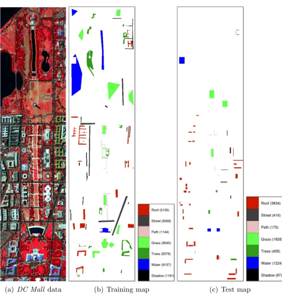
3.1 False color image of the DC Mall data set (generated using the bands 63, 52 and 36) and the corresponding ground truth maps for training and testing. (Images taken from [3].) . . . 14 3.2 False color image of the Centre data set (generated using the bands

68, 30 and 2) and the corresponding ground truth maps for training and testing. (Images taken from [3].) . . . 15 3.3 False color image of the University data set (generated using the

bands 68, 30 and 2) and the corresponding ground truth maps for training and testing. (Images taken from [3].) . . . 17 3.4 Gabor texture filters at different scales (s = 1, . . . , 4) and

orienta-tions (o ∈ {0◦, 45◦, 90◦, 135◦}). (Image taken from [3].) . . . 18 3.5 Pixel feature examples for the DC Mall data set. (Images taken

from [3].) . . . 19

LIST OF FIGURES xi

3.6 Pixel feature examples for the Centre data set. (Images taken from [3].) . . . 20 3.7 Pixel feature examples for the University data set. (Images taken

from [3].) . . . 21

4.1 Opening and closing by reconstruction example. . . 24 4.2 The morphological opening profile and the derivative of the

mor-phological opening profile example. . . 25 4.3 Example region obtained by Pesaresi and Benediktsson’s approach

[54]. . . 27 4.4 Example pixels whose DMP are greater than 0. . . 29 4.5 Example connected components for a building structure. . . 30 4.6 Example connected components appearing for SE sizes from 2 to

10 in the derivative of the opening profile of the 3rd PCA band. . 31 4.7 An example tree. . . 32 4.8 An example tree where each candidate region is a node. . . 33 4.9 An example run of Bottom-Up algorithm on the tree in Figure 4.7. 38 4.10 An example run of Top-Down algorithm on the tree in Figure 4.9(d). 39

5.1 Example segmentation results (overlaid as white on false color and zoomed) for the DC Mall data set. . . 41 5.2 Example segmentation results (overlaid as white on false color and

zoomed) for the Centre data set. . . 41 5.3 A segment modeling example. . . 43

LIST OF FIGURES xii

5.4 PLSA graphical model. . . 44

6.1 An example hierarchical framework for analyzing the image. . . . 48

6.2 Multi-scale segmentation example. . . 49

7.1 Example segmentation results for the DC Mall data set. . . 53

7.2 Example segmentation results for the Centre data set. . . 54

7.3 Example segmentation results for the University data set. . . 55

7.4 Examples of object detection for the DC Mall data set. . . 58

7.5 Examples of object detection for the Centre data set. . . 59

7.6 Examples of object detection for the University data set. . . 60

7.7 Final classification maps with the region level classifier and the quadratic Gaussian classifier for the DC Mall data set. . . 63

7.8 Final classification maps with the region level classifier and the quadratic Gaussian classifier for the Centre data set. . . 64

7.9 Final classification maps with the region level classifier and the quadratic Gaussian classifier for the University data set. . . 64

List of Tables

7.1 Precision values on three object types from the DC Mall data set. 57 7.2 Confusion matrix when region features were used with the decision

tree classifier for the DC Mall data set (testing subset). Classes were listed in Fig. 3.1. . . 62 7.3 Confusion matrix when region features were used with the decision

tree classifier for the Centre data set (testing subset). Classes were listed in Fig. 3.2. . . 62 7.4 Confusion matrix when region features were used with the decision

tree classifier for the University data set (testing subset). Classes were listed in Fig. 3.3. . . 62 7.5 Summary of classification accuracies using the region level classifier

and the quadratic Gaussian classifier. . . 63

Chapter 1

Introduction

1.1

Overview

Due to the constantly increasing public availability of high-resolution data sets, remote sensing image analysis has been an important research area for the last four decades. For example, nearly 3 terabytes of data are being sent to Earth by NASA’s satellites every day [24]. There is also an extensive literature on classifi-cation of remotely sensed imagery using parametric or nonparametric statistical or structural techniques [47]. Advances in satellite technology and computing power have enabled the study of multi-modal, multi-spectral, multi-resolution and multi-temporal data sets for applications such as urban land use monitor-ing and management, GIS and mappmonitor-ing, environmental change, site suitability, agricultural and ecological studies.

The usual choice for the level of processing image data has been pixel-based analysis in both academic and commercial remote sensing image analysis systems. However, a recent study [74] that investigated classification accuracies reported in the last 15 years showed that there has not been any significant improvement in the performance of classification methodologies over this period. We believe that the reason behind this problem is the fact that there is a large semantic gap

CHAPTER 1. INTRODUCTION 2

between the low-level features used for classification and the high-level expecta-tions and scenarios required by the users. This semantic gap makes a human expert’s involvement and interpretation in the final analysis inevitable and this makes processing of data in large remote sensing archives practically impossible. The use of only pixel level features often does not meet the expectations as the resolution increases. Even though high success rates have been published in the literature using limited ground truth data, visual inspection of the results can show that most of the urban structures still cannot be delineated as accurately as expected. For example, if there is an area crowded by buildings in an image, classifying most of the pixels in that area as building while missing most of the roads and other small structures around them will still result in a high success rate if limited amount of pixel level ground truth is used for evaluation. In Figure 1.1, an example classification map with a pixel level quadratic Gaussian classifier is shown [3]. The classification accuracy is 93.9677% which is relatively high. However, most of the tiles on the left are merged, the boundaries are not explicit, and the thin asphalts and shadows between the tiles are also classified as tiles. These erroneous areas are not reflected in the numerical accuracy since the ground truth for testing such areas is not enough for a reliable evaluation. For example, no testing data for these thin roads and shadows are available. So, classifying these areas erroneously does not reduce the numerical classification accuracy. In Figure 1.2, an example classification map obtained in a recent study is shown [9]. The classification accuracy is 98.5% which is also relatively high. However, the classification map includes many wrongly classified pixels for all classes such as the roads and water on the upper part. The same reason also holds for this disagreement between the quantitative accuracy and the qualitative result such that testing data is insufficient for reliable evaluation.

The commonly used classifiers model image content using distributions of pixels in spectral or other feature domains by assuming that similar land cover structures will cluster together and behave similarly in these feature spaces. How-ever, the assumptions for distribution models often do not hold for different kinds of data. Even when nonlinear tools such as neural networks or multi-classifier sys-tems are used, the use of only pixel-based data often fails the expectations.

CHAPTER 1. INTRODUCTION 3

(a) False-color (b) Classification map

Figure 1.1: An example classification map with a pixel level quadratic Gaussian classifier for the Centre data set whose false color image is shown on the left. The corresponding ground truth maps for training and testing and class color codes are listed in Figure 3.2. (Images taken from [3].)

CHAPTER 1. INTRODUCTION 4

(a) False-color (b) Ground truth (c) Classification map

Figure 1.2: An example classification map (shown in (c)) obtained by a recent method [9] for the DC Mall data set whose false color image is shown in (a). The corresponding ground truth map and class color codes are listed in (b). 40 samples per class were used for training and the remaining were used for testing. (Images taken from [9].)

CHAPTER 1. INTRODUCTION 5

We believe that spatial and structural information should also be used for more intuitive and accurate classification. However, image segmentation is still an unsolved problem. Even though several approaches such as region growing, Markov random field models, and energy minimization have been shown to be useful in small data sets with limited detail, no generally applicable segmentation algorithm exists.

In this thesis, first, we describe a segmentation method for remote sensing images that uses the neighborhood and spectral information as well as the mor-phological information. First, principal components analysis (PCA) [23] is per-formed to extract the top principal components that represent the 99% variance of the whole data. Next, morphological opening/closing by reconstruction oper-ations are performed on each PCA band separately using structuring elements in increasing sizes. These operations produce a set of connected components form-ing a hierarchy of regions for each PCA band. Then, the components at different levels of the hierarchy are evaluated as candidates for meaningful structures using a measure that consists of two factors: spectral homogeneity, which is calculated in terms of variances of multi-spectral features, and neighborhood connectivity, which is calculated using sizes of connected components. Finally, the components that optimize this measure are selected as meaningful structures in the image.

Then, we propose an unsupervised method for automatic selection of con-nected components corresponding to meaningful structures among a set of can-didate regions from multiple PCA bands. Given multiple objects/structures of interest, the problem is seen as a grouping problem. To solve the grouping prob-lem, we use the probabilistic Latent Semantic Analysis (PLSA) [37] technique which uses a graphical model for the joint probability of the regions and their features in terms of the probability of observing a feature given an object and the probability of an object given the region. The parameters of this graphical model are learned using the Expectation-Maximization algorithm. Then, for a particular region, the set of probabilities of objects/structures given this region can be used to assign an object label to this region.

CHAPTER 1. INTRODUCTION 6

using spatial information extracted from multi-scale segmentations. First, the proposed segmentation algorithm is applied using multiple disjoint structuring element size ranges corresponding to different scales. As the scale increases, the structuring elements gets larger in order first to capture the details and then the general image context. The resulting segments are modeled by their pixel prop-erties, clustered by using the proposed object detection algorithm and classified according to their cluster labels. Final classification is done using decision tree classifiers.

1.2

Summary of Contributions

The goal of this thesis is to analyze remote sensing images and classify objects into land cover/use classes (e.g., buildings, trees, roads, etc.). The classification process is used as a crucial step to interpret the land in many different kinds of applications.

Today’s trend in classification of remote sensing images is to do object-oriented classification rather than classifying single pixels. This requires segmentation of objects before assigning their class labels. Most of the previous segmentation work in the remote sensing literature are based on merging neighboring pixels according to user-defined thresholds on their spectral similarity. In this work, the approach we follow is to incorporate structural and shape information in the segmentation step. There are several approaches for extraction of these structures from the image data. However, most of the previous approaches try to solve the problem on specific images such as images of the same type of area and images where these structures are isolated. Our goal is to develop a generic model that can be applied to different types of images.

Seen from this aspect, [54] is related to our work in terms of using structural information in segmentation. In that work, Pesaresi and Benediktsson used mor-phological processing, which has recently become a popular approach for remote

CHAPTER 1. INTRODUCTION 7

sensing image analysis, in order to obtain structural information. They success-fully applied opening and closing operations with increasing structuring element sizes to an image to generate morphological profiles for all pixels, and assigned a segment label to each pixel using the structuring element size corresponding to the largest derivative of these profiles. Even though morphological profiles are sensitive to different pixel neighborhoods, the segmentation decision is per-formed by evaluating pixels individually without considering the neighborhood information, and the assumption that all pixels in a structure have only one signif-icant derivative maximum occurring at the same structuring element size may not always hold. However, different than that work, our method [2] uses morphologi-cal, neighborhood and spectral information at the same time to segment images. Morphological and neighborhood information are used to determine hierarchical candidate regions for the final segmentation. Then, the meaningful regions in the hierarchy are selected by testing the goodness of each candidate. In a previous work [66], the selection was done in a segmentation hierarchy manually. In this work, we do the selection process automatically by defining a measure for each candidate region and selecting the regions optimizing the measure.

Our object detection method [1] automatically selects meaningful structures among a set of candidate regions from multiple segmentations using probabilistic Latent Semantic Analysis (PLSA). PLSA was originally developed for statistical text analysis to discover topics in a collection of documents that are represented using the frequencies of words from a vocabulary. In our case, the documents correspond to image segments, the word frequencies correspond to histograms of pixel-level features computed as region-level features, and the topics to be discovered correspond to the set of objects/structures of interest in the image. Note that the whole learning and grouping algorithm proceeds in an unsuper-vised fashion. Russell et al. [58] used a different graphical model in a similar setting where multiple segmentations of natural images were obtained using the normalized cut algorithm by changing its parameters, and instances of regions corresponding to objects such as cars, bicycles, faces, sky, etc. were successfully grouped and retrieved from a large data set of images.

CHAPTER 1. INTRODUCTION 8

on our segmentation and object detection algorithms. Instead of classifying sin-gle pixels according to their spectral properties, we classify regions according to the statistical summary of their pixel properties. We model image content by obtaining segmentations in multiple scales. A recent similar approach [14] also did multi-scale region based classification. They obtained multiple hierarchical segmentations by applying region merging with different thresholds on spectral similarities. However, region merging-based methods work randomly and thresh-olding on spectral similarities does not effectively take into account the structural and shape information. Our method overcomes these disadvantages by the multi-scale nature of our segmentation algorithm. We obtain segmentations in multiple scales by applying the segmentation algorithm with successive disjoint structuring element size ranges.

1.3

Organization of the Thesis

The rest of the thesis is organized as follows. In Chapter 2, some of the pre-vious work on remote sensing image classification is discussed. In Chapter 3, data and features used are introduced. In Chapter 4, a segmentation method for high-resolution remote sensing imagery is presented. For this purpose, a hierar-chical segmentation tree is constructed by using both morphological and spectral information. In Chapter 5, a statistical method for unsupervised detection of objects in high-resolution remote sensing imagery is presented. The method uses the proposed segmentation method to find coherent groups of segments corre-sponding to objects from a set of hierarchical segmentations. In chapter 6, a multi-scale region-based approach for supervised classification of remotely sensed imagery is presented. The method constructs a scale-space by applying the pro-posed segmentation method in different scales. Then, a new set of features is formed by clustering the segments in multiple scales by the proposed object de-tection method. In Chapter 7, experiments are discussed. Finally, in Chapter 8, conclusions and future research directions are given.

Chapter 2

Literature Review

As the amount of data to use increases day-by-day, content extraction and clas-sification of remotely sensed imagery have become important research prob-lems. Previous approaches modeled image content using only pixel level features whereas, today, techniques to incorporate spatial information into land cover/use interpretation have gained importance. In this chapter, we discuss some of the previous work on land cover/use classification. For better understandability, we divide the discussion into two categories: Pixel level techniques and spatial tech-niques using context.

2.1

Pixel Level Techniques

There is an extensive literature on pixel-level analysis of remotely sensed im-agery [47]. In remote sensing images, a pixel may correspond to a large area covering different types of objects such as buildings, roads, shadows, grass, and trees [70]. For example, in a Landsat image, the characteristics of a 225 m2 _area

are summarized in a pixel which may cause problems in pixel-level approaches. Pixel level techniques performs classification using distribution of pixels in spec-tral or other feature domains assuming that similar land structures will cluster

CHAPTER 2. LITERATURE REVIEW 10

together and behave similarly in terms of summarized pixel level features. How-ever, the assumptions for distribution models often do not hold for high-resolution data. In literature, traditional classifiers such as the maximum likelihood method [28, 11], n-dimensional probability density methods [15], artificial neural networks [29, 75, 13, 36, 7, 53, 61, 40, 38, 22], decision trees [31, 43], discriminant analysis [26, 27], genetic algorithms [69, 8] have been applied by using pixel-level infor-mation. However, these methods could not exceed a certain level in terms of accuracy rates.

A remote sensing image may have many feature bands corresponding to dif-ferent wavelengths. For example, a multi-spectral image may have 4 to 7 bands, whereas a hyper-spectral image may have up to 240 bands [70]. The use of hyper-spectral data in classification has been studied in several works [20, 57]. However, most of the hyper-spectral bands are generally correlated and not use-ful for classification. Different methods, such as principal components analysis [34, 39, 45, 56, 44, 9], discriminant analysis feature extraction (DAFE) [47], the decision boundary feature extraction (DBFE) [47], feature selection [52, 68] and spectral unmixing [19, 17, 18, 63, 57, 16, 72], have been applied to reduce the dimensionality.

Even though pixel level techniques were popular when resolution was not high enough for applying other techniques [70], pixels alone do not give much information about image content as the resolution increases because they do not take into account contextual information during the labeling process. In general, the techniques that can be used for a better classification require the use of spatial and neighborhood information.

2.2

Spatial Techniques Using Context

We believe that, in addition to pixel-based spectral data, structural and spatial information should also be used to interpret land cover and land use. Tradition-ally, this is done by the use of textural, morphological, and region level features.

CHAPTER 2. LITERATURE REVIEW 11

In literature, textural features, such as grey-level co-occurrence matrix (GLCM) [32, 64], normalized gray-level run lengths [73], or Markov random fields (MRF) [21], have been widely used to model spatial information. Li and Narayanan [48] used Gabor wavelet coefficients to characterize spatial informa-tion. In a recent approach, Bhagavathy and Manjunath [12] used Gabor texture filters with different scales and orientations, and performed Gaussian mixture-based clustering of pixels as texture elements. In another study, Shackelford and Davis [62] used texture measures extracted form normalized gray-level histogram, contextual and spectral information for classification of urban areas. In [76], Yu et al. extracted gradient based features for urban area detection. Unsalan and Boyer [71] modeled image windows by using edge information for urbanization detection. However, instead of modeling spatial context by pixel windows, an image segmentation approach may further improve the classification results.

Morphological processing has recently become a popular approach for incor-porating structural information into classification. For example, Benediktsson et al. [10] applied morphological operators with different structuring element sizes to obtain a multi-scale representation of structural information, and used neural network classifiers to label pixels according to their morphological profiles. Each pixel feature was obtained as the difference between the multi-scale morphological profiles at successive scales.

Another method for incorporating spatial information into classification is through the use of regions obtained by segmentation. This is also referred to as object-oriented classification in the remote sensing literature. Image segmenta-tion techniques [33] automatically group neighboring pixels into contiguous re-gions whose pixels are similar in terms of a criteria. Although image segmentation is heavily studied in computer vision and image processing fields, and despite the early efforts [42] that use spatial information for classification of remotely sensed imagery, segmentation algorithms have only recently started receiving emphasis in remote sensing image analysis. Examples of image segmentation in the remote sensing literature include region growing [25] and Markov random field models [60] for segmentation of natural scenes, hierarchical segmentation for image mining

CHAPTER 2. LITERATURE REVIEW 12

[67], region growing for object level change detection [35], and boundary delin-eation of agricultural fields [59]. However, better segmentation of regions will definitely improve the object-oriented classification results. Most of the previous classification work use segmentation as a preprocess for incorporating spatial in-formation. But, in general, simple and unreliable segmentation algorithms are ap-plied. In [46], Kusaka and Kawata used an edge-based segmentation technique to find uniform regions, and classified these regions based on their spectral and spa-tial features. Bruzzone and Carlin [14] performed classification using the spaspa-tial context of each pixel according to a complete hierarchical multi-level representa-tion of the scene. Their system was made up of a feature extracrepresenta-tion module and a classifier. They applied a region merging-based hierarchical segmentation to the images to obtain segmentation results at different levels of resolution. Then, each pixel was characterized by a feature vector that included both the pixel level spectral information and the attributes of all the regions in which the pixel was included in the hierarchical segmentation. In a similar approach [4], we obtained a multi-resolution representation using wavelet decomposition [50, 49], segmented images at each resolution using clustering and mathematical morphology-based segmentation algorithms, and used region-based spectral, textural and shape fea-tures for classification. In [41], Katartzis et al. also modeled spatial information by segmenting images into regions and classifying these regions. Their system was based on a Markovian model, defined on the hierarchy of a multiscale region adjacency graph. In another study [65], Soh et al. presented a system for sea ice image classification which also segments the images, generate descriptors for the segments and then uses expert system rules to classify the images.

Chapter 3

Feature Extraction and Datasets

The algorithms presented in this thesis will be illustrated using three different data sets:

1. DC Mall : HYDICE (Hyperspectral Digital Image Collection Experiment) image with 1, 280 × 307 pixels and 191 spectral bands corresponding to an airborne data flightline over the Washington DC Mall area.

The DC Mall data set includes 7 land cover/use classes: roof, street, path, grass, trees, water, and shadow. A thematic map with ground truth labels for 8,079 pixels was supplied with the original data [47]. We used this ground truth for testing and separately labeled 35,289 pixels for training. Details are given in Figure 3.1.

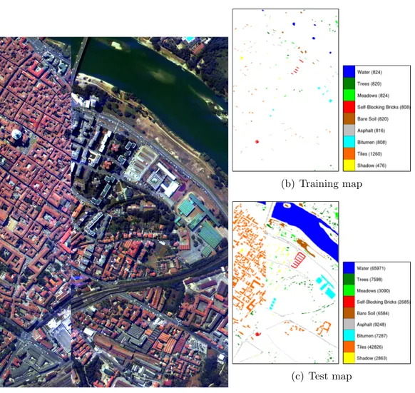
2. Centre: DAIS (Digital Airborne Imaging Spectrometer) and ROSIS (Re-flective Optics System Imaging Spectrometer) data with 1, 096 × 715 pixels and 102 spectral bands corresponding to the city center in Pavia, Italy. The Centre data set includes 9 land cover/use classes: water, trees, mead-ows, self-blocking bricks, bare soil, asphalt, bitumen, tiles, and shadow. The thematic maps for ground truth contain 7,456 pixels for training and 148,152 pixels for testing. Details are given in Figure 3.2.

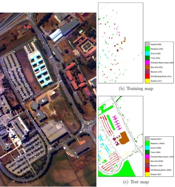
3. University: DAIS and ROSIS data with 610 × 340 pixels and 103 spectral 13

CHAPTER 3. FEATURE EXTRACTION AND DATASETS 14

(a) DC Mall data (b) Training map (c) Test map

Figure 3.1: False color image of the DC Mall data set (generated using the bands 63, 52 and 36) and the corresponding ground truth maps for training and testing. The number of pixels for each class are shown in parenthesis in the legend. (Images taken from [3].)

CHAPTER 3. FEATURE EXTRACTION AND DATASETS 15

(a) Centre data

(b) Training map

(c) Test map

Figure 3.2: False color image of the Centre data set (generated using the bands 68, 30 and 2) and the corresponding ground truth maps for training and testing. The number of pixels for each class are shown in parenthesis in the legend. (A missing vertical section in the middle was removed.) (Images taken from [3].)

CHAPTER 3. FEATURE EXTRACTION AND DATASETS 16

bands corresponding to a scene over the University of Pavia, Italy.

The University data set also includes 9 land cover/use classes: asphalt, meadows, gravel, trees, (painted) metal sheets, bare soil, bitumen, self-blocking bricks, and shadow. The thematic maps for ground truth contain 3,921 pixels for training and 42,776 pixels for testing. Details are given in Figure 3.3.

In the rest of the chapter, pixel level characterization consists of spectral and textural properties of pixels that are extracted as described below.

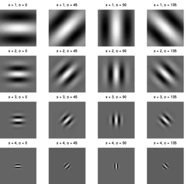
To simplify computations and to avoid the curse of dimensionality during the analysis of hyper-spectral data, we apply Fisher’s linear discriminant analysis (LDA) [23] that finds a projection to a new set of bases that best separate the data in a least-squares sense. The resulting number of bands for each data set is one less than the number of classes in the ground truth. We also apply principal components analysis (PCA) [23] that finds a projection to a new set of bases that best represent the data in a least-squares sense. Then, we keep the top principal components representing the 99% variance of the whole data instead of the large number of hyper-spectral bands. The resulting number of bands for DC Mall, Centre and University data sets are 3, 3 and 4, respectively. In addition, we extract Gabor texture features [51] by filtering the first principal component image with Gabor kernels at different scales and orientations shown in Figure 3.4. We use kernels rotated by nπ/4, n = 0, . . . , 3, at 4 scales resulting in feature vectors of length 16.

Finally, each feature component is normalized by linear scaling to unit variance [5] as

˜

x = x − µ

σ (3.1)

where x is the original feature value, ˜x is the normalized value, µ is the sample mean, and σ is the sample standard deviation of that feature, so that the features with larger ranges do not bias the results. Examples for pixel level features are shown in Figures 3.5-3.7.

CHAPTER 3. FEATURE EXTRACTION AND DATASETS 17

(a) University data

(b) Training map

(c) Test map

Figure 3.3: False color image of the University data set (generated using the bands 68, 30 and 2) and the corresponding ground truth maps for training and testing. The number of pixels for each class are shown in parenthesis in the legend. (Images taken from [3].)

CHAPTER 3. FEATURE EXTRACTION AND DATASETS 18

Figure 3.4: Gabor texture filters at different scales (s = 1, . . . , 4) and orientations (o ∈ {0◦, 45◦, 90◦, 135◦}). Each filter is approximated using 31×31 pixels. (Image taken from [3].)

CHAPTER 3. FEATURE EXTRACTION AND DATASETS 19

Figure 3.5: Pixel feature examples for the DC Mall data set. From left to right: the first LDA band, the first PCA band, Gabor features for 90 degree orientation at the first scale, Gabor features for 0 degree orientation at the third scale, and Gabor features for 45 degree orientation at the fourth scale. Histogram equal-ization was applied to all images for better visualequal-ization. (Images taken from [3].)

CHAPTER 3. FEATURE EXTRACTION AND DATASETS 20

Figure 3.6: Pixel feature examples for the Centre data set. From left to right, first row: the first LDA band, the first PCA band, Gabor features for 135 degree orientation at the first scale; second row: Gabor features for 45 degree orientation at the third scale, Gabor features for 45 degree orientation at the fourth scale, and Gabor features for 135 degree orientation at the fourth scale. Histogram equalization was applied to all images for better visualization. (Images taken from [3].)

CHAPTER 3. FEATURE EXTRACTION AND DATASETS 21

Figure 3.7: Pixel feature examples for the University data set. From left to right, first row: the first LDA band, the first PCA band, Gabor features for 45 degree orientation at the first scale; second row: Gabor features for 45 degree orientation at the third scale, Gabor features for 135 degree orientation at the third scale, and Gabor features for 135 degree orientation at the fourth scale. Histogram equalization was applied to all images for better visualization. (Images taken from [3].)

Chapter 4

Image Segmentation

In this work, our goal is to develop a segmentation algorithm for partitioning images into spatially contiguous regions so that the structural information can be modeled using the properties of these regions in classification. Many popular image segmentation algorithms in the computer vision literature that are based on clustering assume that images have a moderate number of objects with rel-atively homogeneous features, and cannot be directly applied to high-resolution remote sensing images that contain a large number of complex structures. Fur-thermore, another popular approach of edge-based segmentation becomes hard for such images because of the large amount of details. Moreover, watershed-based techniques are also not very useful because they often produce oversegmented re-sults mostly because of irrelevant local extrema in images. A common approach is to apply smoothing filters to suppress these extrema but lots of details in high-resolution images may be lost because spatial support of these details are usually small. Therefore, most of the segmentation work in the remote sensing literature are based on merging neighboring pixels according to user-defined thresholds on their spectral similarity. As an alternative, proximity filtering and morphological operations can also be used as post-processing techniques to pixel-based classifi-cation results for segmenting regions [6].

In a related work, Pesaresi and Benediktsson [54] performed segmentation us-ing morphological characteristic of pixels in the image. In their approach, openus-ing

CHAPTER 4. IMAGE SEGMENTATION 23

and closing operations with increasing structuring element (SE) sizes were suc-cessively applied to an image to generate morphological profiles for all pixels, and the segment label of each pixel was assigned as the SE size corresponding to the largest derivative of these profiles. A problem with that approach is that it assumes all the pixels in a particular structure have only one significant deriva-tive maximum occurring at the same SE size. However, our experiments have shown that many pixels in most structures often have more than one significant derivative maximum. Furthermore, even though morphological profiles are sensi-tive to different pixel neighborhoods, the segmentation decision is performed by evaluating pixels individually without considering the neighborhood information. In this chapter, we present a method that uses the neighborhood and spectral information as well as the morphological information. We first apply principal components analysis to hyper-spectral data to obtain representative bands. Then, we extract candidate regions on each principal component by applying opening and closing by reconstruction operations. For each principal component, we rep-resent the extracted regions by a hierarchical tree, and select the most meaningful regions in that tree by optimizing a measure that consists of two factors: spectral homogeneity, which is calculated in terms of variances of multi-spectral features, and neighborhood connectivity, which is calculated using sizes of connected com-ponents.

4.1

Morphological Profiles

Morphological opening and closing operations are used to model structural char-acteristics of pixel neighborhoods. These operations are known to isolate struc-tures that are brighter and darker than their surroundings, respectively. Contrary to opening (respectively, closing), opening by reconstruction (respectively, clos-ing by reconstruction) preserves the shape of the structures that are not removed by erosion (respectively, dilation). In other words, image structures that the SE cannot be contained are removed while others remain (see Figure 4.1 for an illustration).

CHAPTER 4. IMAGE SEGMENTATION 24

(a) Gray-scale image (b) SE

(c) 3-d representation of (a) (d) After opening by recon-struction

(e) After closing by recon-struction

Figure 4.1: Opening and closing by reconstruction example. (d) and (e), respec-tively, show 3-d representations of the results of opening and closing by recon-struction applied on (a) with a disk SE of size 5. In (d) and (e), respectively, brighter and darker image structures that the SE cannot be contained are removed by flattening the pixels on the structure into same level.

CHAPTER 4. IMAGE SEGMENTATION 25

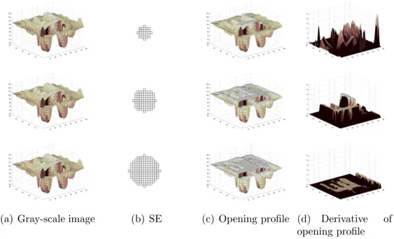
(a) Gray-scale image (b) SE (c) Opening profile (d) Derivative of opening profile

Figure 4.2: The morphological opening profile and the derivative of the morpho-logical opening profile example. The original image in (a) is applied opening by reconstruction with increasing SE sizes (disk SEs of sizes 3, 5 and 7 are used as shown in (b)) to obtain the opening profile in (c). The difference between consecutive steps of the opening profile is stored as the derivative of the opening profile as shown in (d).

These operations are applied using increasing SE sizes to generate multi-scale characteristics called morphological profiles For completeness, we review the con-cepts of the morphological profile and the derivative of the morphological profile as defined by Pesaresi and Benediktsson [54] below (see Figure 4.2 for an illus-tration).

Let γλ be the morphological opening by reconstruction operator using SE with

size λ (in our case λ represents the radius of a disk shaped SE) and Πγ(x) denote

the opening profile at pixel x of image I. Πγ(x) is defined as the vector

Πγ(x) = {Πγλ : Πγλ = γλ(x), ∀λ ∈ [0, . . . , m]}. (4.1)

Also, let ϕλ be the morphological closing by reconstruction operator using SE

with size λ and Πϕ(x) denote the closing profile at pixel x of image I. Similarly,

Πϕ(x) is defined as the vector

CHAPTER 4. IMAGE SEGMENTATION 26

The definition of opening and closing by reconstruction operations imply that Πγ0(x) = Πϕ0(x) = I(x). The derivative of the morphological profile (DMP) is

defined as a vector where the measure of the slope of the opening-closing profile is stored for every step of an increasing SE series [54]. The derivative of the opening profile ∆γ(x) is defined as the vector

∆γ(x) = {∆γλ : ∆γλ = |Πγλ− Πγλ−1|, ∀λ ∈ [1, . . . , m]}. (4.3)

Similarly, the derivative of the closing profile ∆ϕ(x) is defined as the vector

∆ϕ(x) = {∆ϕλ : ∆ϕλ = |Πϕλ− Πϕλ−1|, ∀λ ∈ [1, . . . , m]}. (4.4)

Then, the DMP ∆(x) can be written as the vector ∆(x) = ( ∆c+λ: ∆γλ, ∀λ ∈ [1, . . . , m] ∆c−λ+1 : ∆ϕλ, ∀λ ∈ [1, . . . , m] ) (4.5) for an arbitrary integer c with m equal to the total number of iterations [54].

In their segmentation scheme, Pesaresi and Benediktsson [54] define an image segment as a set of connected pixels showing the greatest value of the DMP for the same SE size. That is, the segment label of each pixel is assigned according to the SE size corresponding to the largest derivative of its profiles. Their scheme works well in images where the structures in the image are mostly flat so that all pixels in a structure have only one derivative maximum. A drawback of this scheme is that neighborhood information is not used while assigning segment labels to pixels. This results in lots of small noisy segments in images with non-flat structures where the scale with the largest value of the DMP may not correspond to the true structure (see Figure 4.3 for an illustration). In our approach, we do not consider pixels alone while assigning segment labels. Instead, we also take into account the behavior of the neighbors of the pixels.

4.2

Hierarchical Region Extraction

In our segmentation approach, our aim is to determine the regions by applying opening and closing by reconstruction operations. We assume that pixels with a

CHAPTER 4. IMAGE SEGMENTATION 27

(a) DMP of the pixel marked in (b)

(b) Sample pixel marked on the image

(c) Region for SE size 2 (d) Region for SE size 3

Figure 4.3: The greatest value in the DMP of the pixel marked with a blue + in (b) is obtained for SE size 2 (derivative of the opening profile of the 3rd PCA band is shown in (a)). (c) shows the region that we would obtain if we label the pixels with the SE size corresponding to the greatest DMP. The region in (d) that occurs with SE size 3 is more preferable as a complete structure but it does not correspond to the scale of the greatest DMP for all pixels inside the region.

CHAPTER 4. IMAGE SEGMENTATION 28

positive DMP value at a particular SE size face a change with respect to their neighborhoods at that scale. The main idea is that a neighboring group of pix-els that have a similar change for a particular SE size is a candidate region for the final segmentation. These groups can be found by applying connected com-ponents analysis to the DMP at each scale (see Figure 4.4 for an illustration). Then, we use the spectral angle mapper (SAM) as a rough measure to check the spectral homogeneity within each group. SAM between two vectors si and

sj is calculated as: SAM (si, sj) = cos−1( si·sj

ksikksjk). Using SAM, spectral

similar-ity of pixel vectors {p}K

i in the region Rk relative to the vector sj is computed

as: S(Rk, sj) = (1/K)PK_i=1SAM (sj, pi) where K is the number of pixels in the

region Rk. Then, Plaza and Tilton [55] define a measure of homogeneity in the

re-gion Rk as: S(Rk, ck) where ck = (1/K)

PK

i=1pi is the centroid of Rk. S indicates

how similar are spectral information of the pixels in a region. The less the S, the more the region is homogeneous. The connected components whose average DMP values are greater than 0.2 and average SAM values are less than 0.095 are considered in the rest of the analysis. These thresholds are chosen empirically.

Considering the fact that different structures have different sizes, we apply opening and closing by reconstruction using SEs in increasing sizes from 1 to m. However, a connected component appearing for a small SE size may be appearing because heterogeneity and geometrical complexity of the scenes as well as other external effects such as shadows produce texture effects in images and result in structures that can be one to two pixels wide [54]. In this case, there is most probably a larger connected component appearing at the scale of a larger SE and to which the pixels of those noise components belong. On the other hand, a connected component that corresponds to a true structure in the final segmentation may also appear as part of another component at larger SE sizes. The reason is that a meaningful connected component may start merging with its surroundings and other connected components after the SE size in which it appears is reached. Figure 4.5 illustrates these cases.

For each opening and closing profile, through increasing SE sizes from 1 to m, each morphological operation reveals connected components that are contained within each other in a hierarchical manner where a pixel may be assigned to

CHAPTER 4. IMAGE SEGMENTATION 29

(a) Opening DMP (b) DM P > 0

Figure 4.4: In (b), the pixels whose DMP (DMP of the 2nd PCA band is shown in (a)) are greater than 0 are shown. Each connected component at each scale is a candidate region for the final segmentation.

CHAPTER 4. IMAGE SEGMENTATION 30

(a) False color image (b) A small connected component that is part of (c)

(c) The preferred connected component (d) A large connected component where (c) started merging with others

Figure 4.5: Example connected components for a building structure. These com-ponents appear for SE sizes 3, 5 and 6, respectively, in the derivative of the opening profile of the 2nd PCA band.

CHAPTER 4. IMAGE SEGMENTATION 31

(a) (b) (c) (d) (e)

(f) (g) (h) (i) (j)

Figure 4.6: Example connected components appearing for SE sizes from 2 to 10 in the derivative of the opening profile of the 3rd PCA band. These regions are contained within each other in a hierarchical manner. Note that the components do not change in some of the scales.

more than one connected component appearing at different SE sizes (see Figure 4.6). We treat each component as a candidate meaningful region. Using these candidate regions, a tree is constructed where each connected component is a node and there is an edge between two nodes corresponding to two consecutive scales (SE sizes differ by 1) if one node is contained within the other. Leaf nodes represent the components that appear for SE size 1. Root nodes represent the components that exist for SE size m. Since we use a finite number of SE sizes, there may be more than one root node. In this case, there will be more than one tree and the algorithms described in the next section are run on each tree separately.

Figure 4.7 shows an example tree where the nodes are labeled as i j with i denoting the node’s level and j denotes the number of the node from left to right in level i. For example, node 3 3 has two children nodes 2 4 and 2 5, and its parent is node 4 1. The reason of node 2 3 having only one child may be that either no new connected component appears in level 2 or node 2 3 is formed by merging of node 1 4 with its surrounding pixels that are not included in any connected component in level 1. The same reasons also hold for node 3 2. Figure 4.8 shows a part of an example tree constructed by candidate meaningful regions

CHAPTER 4. IMAGE SEGMENTATION 32 level 2 level 1 level 3 level 4 (9) (2) (2) 1_2 1_1 (5) 1_3 (4) 1_6(3) 1_7(4) 2_1 (5) (6) 2_3 2_4(2) 2_5(8) 3_1 3_2 (3) 3_3(4) 4_1 (1) 2_2 (5) 1_8 1_5 (3) (1) 1_4

Figure 4.7: An example tree. Node i j is a connected component that exists for SE size i. j denotes the sequence number of the node from left to right in level i. appearing in five levels.

4.3

Region Selection

After forming a tree for each opening and closing profile, our aim is to search for the most meaningful connected components among those appearing at different SE sizes in the segmentation hierarchy. With a similar motivation in [66], Tilton analyzed hierarchical image segmentations and selected the meaningful regions manually. Then, Plaza and Tilton [55] investigated how different spectral, spatial and joint spectral/spatial features of regions change from one level to another in a segmentation hierarchy with the goal of automating the selection process in the future. In this thesis, each node in the tree is treated as a candidate region in the final segmentation, and selection is done automatically as described below.

Ideally, we expect a meaningful region to be as homogeneous as possible. However, in the extreme case, a single pixel is the most homogeneous. Hence, we also want a region to be as large as possible. In general, a region stays almost the same (both in homogeneity and size) for some number of SEs, and then faces a

CHAPTER 4. IMAGE SEGMENTATION 33

Figure 4.8: An example tree where each candidate region is a node. large change at a particular scale either because it merges with its surroundings to make a new structure or because it is completely lost. Consequently, the size we are interested in corresponds to the scale right before this change. In other words, if the nodes on a path in the tree stay homogeneous until some node n, and then the homogeneity is lost in the next level, we say that n corresponds to a meaningful region in the hierarchy.

With this motivation, to check the meaningfulness of a node, we define a measure consisting of two factors: spectral homogeneity, which is calculated in terms of variances of spectral features, and neighborhood connectivity, which is calculated using sizes of connected components. Then, starting from the leaf nodes (level 1) up to the root node (level m), we compute this measure at each node and select a node as a meaningful region if it is the most homogeneous and large enough node on its path in the hierarchy (a path corresponds to the set of nodes from a leaf to the root).

In order to calculate the homogeneity factor in a node, we use the fact that pixels in a correct structure should have not only similar morphological profiles,

CHAPTER 4. IMAGE SEGMENTATION 34

but also similar spectral features. Thus, we calculate the homogeneity of a node as the standard deviation of the spectral information of the pixels in the corre-sponding region where the spectral information of a pixel consists of the PCA components representing the 99% variance of the whole data. However, while examining a node from the leaf up to the root in terms of homogeneity, we do not use the standard deviation of the node directly. Instead, we consider the differ-ence of the standard deviation of that node and its parent. What we expect is a sudden increase in the standard deviation. When the standard deviation does not change much, it usually means that small sets of pixels are added to the region or some noise pixels are cleaned. When there is a large change, it means that the structure merged with a larger structure or it merged with other irrelevant pixels disturbing the homogeneity in the node. Hence, the difference of the standard deviation in the node’s parent and the standard deviation in the node should be maximized while selecting the most meaningful nodes.

To be able to calculate a single value for the difference of the standard de-viations, we must find a single value for the standard deviation of the PCA components of the pixels in a node and its parent. Let the number of PCA com-ponents be d. We find a single standard deviation value for the d-dimensional PCA components X of the pixels in node n by projecting X into a 1-dimensional representation where we find the standard deviation [30]. X is projected onto the vector connecting the average of the PCA components of n and the average of the PCA components of the parent of n. This is the vector where it is believed to be important for separating the data. Let c1 be the average of the PCA

com-ponents of n, c2 be the average of the PCA components of the parent of n, and

v = c1 − c2 be the d-dimensional vector connecting c1 and c2. The projection

xi0 ∈ X0 of PCA components xi ∈ X of each pixel i is done by: xi0 = <x_||v||i,v>2 .

X0 is a 1-dimensional representation of X projected onto v. After projecting the PCA components of a node and its parent into a 1-dimensional representation, the standard deviation of the projected data for each node is found.

However, using only the homogeneity factor will favor small structures be-cause in the extreme case a single pixel is the most homogeneous. To overcome this problem, the number of pixels in the region corresponding to the node is

CHAPTER 4. IMAGE SEGMENTATION 35

introduced as another factor to create a trade-off. As a result, the goodness measure M for a node n is defined as

M (n) = D(n, parent (n)) × C(n) (4.6) where the first term is the standard deviation difference between the node’s parent and itself, and the second term is the number of pixels in the node. The node that is relatively homogeneous and large enough will maximize this measure and will be selected as a meaningful region.

Given the value of the goodness measure for each node, we find the most meaningful regions as follows. Suppose T = (N, E) is the tree with N as the set of nodes and E as the set of edges. The leaf nodes are in level 1 and the root node is at level m. Let P denote the set of all paths from the leaves to the root, and M (n) denote the measure at node n. descendant(n) denotes descendant nodes of node n. We select N∗ ⊆ N as the final segmentation such that

1. ∀a ∈ N∗, ∀b ∈ descendant(a), M (a) ≥ M (b), 2. ∀a ∈ N \ N∗, ∃b ∈ descendant(a) : M (a) < M (b). 3. ∀a, b ∈ N∗, ∀p ∈ P : a ∈ p → b /∈ p, ∀p ∈ P : b ∈ p → a /∈ p, 4. ∀p ∈ P, ∃a ∈ p : a ∈ N∗_,

The first condition requires that any node in N∗ must have a measure greater than all of its descendants. The second condition requires that no node in N \ N∗ has a measure greater than all of its descendants. The third condition requires that any two nodes in N∗ cannot be on the same path (i.e., the corresponding regions cannot overlap). The fourth condition requires that every path must include a node that is in N∗.

CHAPTER 4. IMAGE SEGMENTATION 36

We use a two-pass algorithm for selecting the most meaningful nodes (N∗) in the tree. The bottom-up (first) pass aims to find the nodes whose measure is greater than all of its descendants (condition 1). The algorithm first marks all nodes in level 1. Then, starting from level 2 up to the root level, it checks whether each node in each level has a measure greater than or equal to those of all of its children. The greatest measure, seen so far in each path, is propagated to upper levels so that it is enough to check only the children, rather than all descendants, in order to find whether a node’s measure is greater than or equal to all of its descendants’.

After the bottom-up pass marks all such nodes, the top-down (second) pass seeks to select the nodes satisfying, as well, the remaining conditions (2, 3, 4). It starts by marking all nodes as selected in the root level if they are marked by the bottom-up pass. Then, in each level until the leaf level, the algorithm checks for each node whether it is marked in the bottom-up pass while none of its ancestors is marked. If this condition is satisfied, it marks the node as selected. Finally, the algorithm selects the nodes that are marked as selected in each level as meaningful regions.

Below, we give the algorithm for selecting the most meaningful nodes in the hierarchical tree. In the algorithm, children(n) denotes children nodes of node n.

Algorithm 1 Region Selection Run Bottom-Up algorithm Run Top-Down algorithm for each level l = 1 to m do

for each node n in level l do

select n as a meaningful region if it is marked as selected end for

end for

In order to illustrate an example run of these algorithms, a measure is given, in parenthesis, in each node i j in the example tree of Figure 4.7. After we run the Bottom-Up algorithm, each node 1 j(1 ≤ j ≤ 8) is marked in the beginning of the algorithm. Then, as we move upwards nodes 2 1, 2 2, 2 3, 2 5 in level 2,

CHAPTER 4. IMAGE SEGMENTATION 37

Algorithm 2 Bottom-Up algorithm Mark all nodes in level 1

for each level l = 2 to m do for each node n in level l do

if M (n) ≥ max{M (a)|a ∈ children(n)} then mark n

else

M (n) = max{M (a)|a ∈ children(n)} leave n unmarked

end if end for end for

Algorithm 3 Top-Down algorithm

Mark all nodes in level m as selected if they’re already marked in Bottom-Up for each level l = m − 1 to 1 do

for each node n in level l do

if parent(n) is marked as selected or parent-selected then mark n as parent-selected

else

if parent(n) is not marked in Top-Down and n is not marked in Bottom-Up then leave n unmarked else mark n as selected end if end if end for end for

CHAPTER 4. IMAGE SEGMENTATION 38

(a) Step 1 (b) Step 2

(c) Step 3 (d) Step 4

Figure 4.9: An example run of Bottom-Up algorithm on the tree in Figure 4.7. Beginning from the leaves until the root, the nodes whose measure are greater than all of its descendants (satisfying condition 1) are colored with blue in each step.

nodes 3 1 and 3 2 are marked in level 3 since each of them is greater than or equal to all of its descendants. Then, we run the Top-Down algorithm and mark nodes 3 1, 3 2, 2 5 and 1 5, satisfying the four conditions defined above, as selected. Figures 4.9 and 4.10 show the marked nodes in each step of the Bottom-Up and the Top-Down algorithms. In the Bottom-Up algorithm, the marked nodes are colored with blue and in the Top-Down algorithm, the marked nodes are colored with green.

After selecting the most meaningful connected components in each opening and closing tree separately, the next step is to merge the resulting connected components. The problem occurs when two connected components, where one is selected from the opening tree and the other is selected from the closing tree, intersect. In this case, the intersecting pixels are assigned to the connected com-ponent whose goodness measure is greater.

CHAPTER 4. IMAGE SEGMENTATION 39

(a) Step 1 (b) Step 2

(c) Step 3 (d) Step 4

Figure 4.10: An example run of Top-Down algorithm on the tree in Figure 4.9(d). Beginning from the root until the leaves, the nodes marked in Bottom-Up algo-rithm which satisfy, as well, the remaining conditions (2, 3, 4) are marked with green in each step. When the algorithm ends, the green nodes are selected as the most meaningful nodes in the tree.

Chapter 5

Object Detection

In Chapter 4, we described a method that used the neighborhood and spectral information as well as the morphological information for segmentation. After principal components analysis (PCA), morphological profiles were generated for each PCA band separately. These operations produced a set of connected compo-nents forming a hierarchy of segments for each PCA band. Then, a measure that combined spectral homogeneity and neighborhood connectivity was designed to select meaningful segments at different levels of the hierarchy.

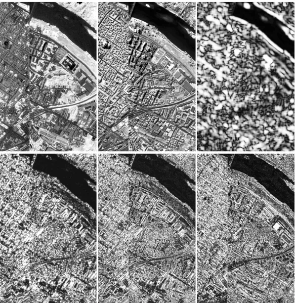
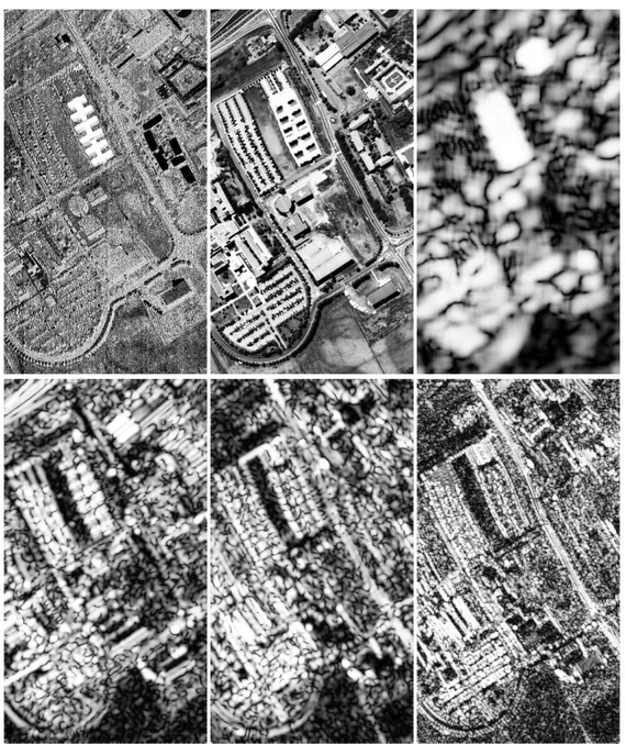
The experiments in Section 7.1 show that the combined measure is able to detect structures in the image that are more precise and more meaningful than the structures detected by the approach in [54]. An important observation is that different structures appear more clearly in different principal components. For example, buildings can be detected accurately in one component but roads, trees, fields and paths can be detected accurately in other components (see Figures 5.1 and 5.2 for examples). Information from multiple PCA components must be combined for better overall detection.

In this chapter, we present an unsupervised algorithm for automatic selection of segments from multiple segmentations and PCA bands. The input to the algo-rithm is a set of hierarchical segmentations corresponding to different PCA bands. The goal is to find coherent groups of segments that correspond to meaningful

CHAPTER 5. OBJECT DETECTION 41

Figure 5.1: Example segmentation results (overlaid as white on false color and zoomed) for the DC Mall data set. The left, middle and right images show the extracted segments in the first, second and third PCA bands, respectively.

Figure 5.2: Example segmentation results (overlaid as white on false color and zoomed) for the Centre data set. The left, middle and right images show the extracted segments in the first, second and third PCA bands, respectively.

CHAPTER 5. OBJECT DETECTION 42

structures. The assumption here is that, for a particular structure (e.g., building), the “good” segments (i.e., the ones containing a building) will all have similar features whereas the “bad” segments (i.e., the ones containing multiple objects or corresponding to overlapping partial object boundaries) will be described by a random mixture of features. Therefore, given multiple objects/structures of interest, this selection process can also be seen as a grouping problem within the space of a large number of candidate segments obtained from multiple segmen-tations. We use the probabilistic Latent Semantic Analysis (PLSA) algorithm [37] to solve the problem. The resulting groups correspond to different types of objects in the image.

5.1

Modeling Segments

The grouping algorithm consists of three steps: extracting segment features, grouping segments, detecting objects. In the first step, each segment is modeled using the statistical summary of its pixel content. First, all pixels in the image are clustered by applying the k-means algorithm [23] in the spectral (PCA, LDA) and textural (Gabor) feature domains. This corresponds to quantization of the feature values. Then, a histogram is constructed for each segment to approxi-mate the distribution of these quantized values belonging to the pixels in that segment. This histogram is used to represent the segment in the rest of the algo-rithm. (Note that any discrete model of the segment’s content can also be used by the grouping algorithm in the next section.)

5.2

Grouping Segments

In this work, we use the probabilistic Latent Semantic Analysis (PLSA) algo-rithm [37] to solve the grouping problem. PLSA was originally developed for statistical text analysis to discover topics in a collection of documents that are represented using the frequencies of words from a vocabulary. In our case, the