AUTOMATED LAYOUT OF PROCESS
DESCRIPTION MAPS DRAWN IN SYSTEMS
BIOLOGY GRAPHICAL NOTATION
a thesis
submitted to the department of computer engineering
and the graduate school of engineering and science
of bilkent university
in partial fulfillment of the requirements
for the degree of
master of science
By
Beg¨
um Gen¸c
I certify that I have read this thesis and that in my opinion it is fully adequate, in scope and in quality, as a thesis for the degree of Master of Science.
Assoc. Prof. Dr. U˘gur Do˘grus¨oz(Advisor)
I certify that I have read this thesis and that in my opinion it is fully adequate, in scope and in quality, as a thesis for the degree of Master of Science.
Asst. Prof. Dr. ¨Oznur Ta¸stan
I certify that I have read this thesis and that in my opinion it is fully adequate, in scope and in quality, as a thesis for the degree of Master of Science.
Asst. Prof. Dr. ¨Ozg¨ur S¸ahin
Approved for the Graduate School of Engineering and Science:
Prof. Dr. Levent Onural Director of the Graduate School
ABSTRACT
AUTOMATED LAYOUT OF PROCESS DESCRIPTION
MAPS DRAWN IN SYSTEMS BIOLOGY GRAPHICAL
NOTATION
Beg¨um Gen¸c
M.S. in Computer Engineering
Supervisor: Assoc. Prof. Dr. U˘gur Do˘grus¨oz July, 2014
Evolving technology has increased the focus on genomics. The combination of today’s advanced studies with decades of molecular biology research yield in huge amount of pathway data. These models can be used to improve high-throughput data analysis by linking correlation to the causation, shedding light on many complex diseases. In order to prevent ambiguity and ensure regularity of the research, a need for using a standard notation has emerged.
Systems Biology Graphical Notation (SBGN) is a visual language developed by a community of biochemists, modellers and computer scientists with the intention of enabling scientists to represent networks, including models of cellular processes, in a standard, unambiguous way. SBGN is formed of three languages: process, entity relationship and activity flow. This research is focused on its process diagram branch.
Automated layout is commonly used to clearly visualize the information repre-sented by graphs. Considering the fact that, biological pathways includes nested structures (e.g., nucleoplasms), we have made use of a force-directed automatic layout algorithm called Compound Spring Embedder (CoSE), which supports the compound graph structures. On top of this layout structure, we have developed a specialized layout algorithm called SBGN-PD layout.
SBGN-PD layout enhancements mainly include properly tiling of complex members and disconnected molecules, placement of product and substrate edges on the opposite sides of a process node without disturbing the force-directed structure of the algorithm.
iv
Keywords: information visualization, graph layout, automatic layout, biological networks, biological process diagrams, graph algorithms, graph visualization, sys-tems biology graphical notation, compound spring embedder.
¨
OZET
SYSTEMS BIOLOGY GRAPHICAL NOTATION
KULLANILARAK C
¸ ˙IZ˙ILEN PROSES
D˙IYAGRAMLARININ OTOMAT˙IK YERLES
¸T˙IRMES˙I
Beg¨um Gen¸c
Bilgisayar M¨uhendisli˘gi, Y¨uksek Lisans Tez Y¨oneticisi: Assoc. Prof. Dr. U˘gur Do˘grus¨oz
Temmuz, 2014
Geli¸sen teknolojiyle birlikte genom bilimi ¨uzerindeki ilgi arttı. G¨un¨um¨uzdeki ileri d¨uzey ¸calı¸smalar ve y¨uzyıllardır s¨uregelen molek¨uler biyoloji ara¸stırmaları birle¸since y¨uksek miktarda yolak verisi olu¸stu. Bu modeller, ba˘gıntıları nedenlere ba˘glayıp, y¨uksek hacimli veri analizinde kullanılarak, bir ¸cok karma¸sık hastalı˘gı aydınlatabilir. Bu ¸calı¸smalardaki anlam belirsizli˘gini ¨onlemek ve d¨uzenlili˘gi sa˘glamak amacıyla standart bir notasyona ihtiya¸c duyuldu.
Systems Biology Graphical Notation (SBGN), bir grup biyokimyacı, mod-elleme uzmanı ve bilgisayar bilimcisi tarafından, bilim adamlarının h¨ucresel s¨ure¸cler de dahil olmak ¨uzere pek ¸cok a˘g yapısını stadart ve belirsizli˘ge yer ver-meyen bir ¸sekilde yansıtması i¸cin geli¸stirilmi¸stir. SBGN ¨u¸c dilden olu¸sur: proses, varlık ili¸ski ve etkinlik akı¸s. Bu ara¸stırma, bu dilin proses diyagramları kolu ¨
uzerine yo˘gunla¸smaktadır.
Otomatik yerle¸stirme, ¸cizgelerle temsil edilen bilginin a¸cık¸ca g¨orselle¸stirilmesini sa˘glamakta yaygın ¸sekilde kullanılır. Biyolojik yolakların i¸ci¸ce yapılar (n¨ukleoplazma vb.) i¸cerdi˘gini g¨oz ¨on¨unde bulundurarak, bu yapıları destekleyen kuvvet-y¨onlendirilmi¸s bir otomatik yerle¸stirme metodu olan Compound Spring Embedder (CoSE) algoritmasını kullandık. Bu algoritma yapısını kullanarak, ¨
ozelle¸stirilmi¸s bir SBGN-PD yerle¸stirme algoritması geli¸stirdik.
SBGN-PD yerle¸stirme algoritması genel olarak; kompleks ¨uyelerinin ve ba˘glantısı olmayan molek¨ullerin d¨uzg¨unce d¨o¸senmesi, proses d¨u˘g¨umlerinin substrat ve ¨ur¨un ba˘glantılarının, ilgili proses d¨u˘g¨umlerinin zıt taraflarına yerle¸stirilmesi ve bu i¸slemlerin algoritmanın kuvvet-y¨onlendirilmi¸s yapısını boz-madan yapılmasını i¸cerir.
vi
Anahtar s¨ozc¨ukler : bilgi g¨orselle¸stirme, ¸cizge yerle¸stirme, otomatik yerle¸stirme, biyolojik a˘g diyagramları, biyolojik proses diyagramları, ¸cizge algoritmaları, ¸cizge g¨orselle¸stirme.
Acknowledgement
I would like to express my gratitude and thanks to my supervisor U˘gur Do˘grus¨oz for the understanding, patience and expertise through the learning process of this master thesis. His supports and advices are greatly appreciated.
Besides my supervisor, I would like to thank to the rest of my thesis committee: Asst. Prof. Dr. ¨Oznur Ta¸stan and Asst. Prof. Dr. ¨Ozg¨ur S¸ahin for reviewing my work and the questions.
Furthermore, I would like to thank to my friends Mecit Sarı, Do˘gukan C¸ a˘gatay, Merve C¸ akır, ˙Istemi Rahman Bah¸ceci, Can C¸ a˘gda¸s Cengiz and Muhsin Can Orhan for the valuable friendship and coffee breaks.
Of course I would like to thank my mom and dad for unconditional support throughout my degree, Selen for being such an understanding sister and Arya for being a charming niece. A very special thanks goes to my brother Burkay Gen¸c, without whose encouragement and assistance, I would have not finished this thesis.
Finally, I would like to thank T ¨UB˙ITAK for making this research possible by providing financial assistance.
Contents
1 Introduction 1
1.1 Motivation . . . 1
1.2 Contribution . . . 5
2 Background and Related Work 7 2.1 Graphs . . . 7
2.2 Systems Biology Graphical Notation . . . 9
2.3 Automated Layout . . . 11
2.4 Compound Spring Embedder . . . 14
2.4.1 CoSE Layout Structure . . . 18
2.5 Rectangle Packing . . . 21
2.5.1 Tiling . . . 23
2.5.2 Polyomino Packing . . . 24
2.6 Compaction . . . 26
CONTENTS ix
3.1 Nested Rectangle Packing . . . 31
3.1.1 Packing Complex Members . . . 33
3.1.2 Packing Non-Complex Members . . . 37
3.1.3 Performing Compaction . . . 40
3.2 Handling Port Nodes . . . 42
3.3 Orienting Products and Substrates . . . 45
4 Results 50 4.1 Evaluation . . . 62
List of Figures
1.1 “ATM mediated phosphorylation of repair proteins” biological net-work shown in Pathway Commons [1] . . . 2 1.2 Visualized version of ATM mediated phosphorylation of repair
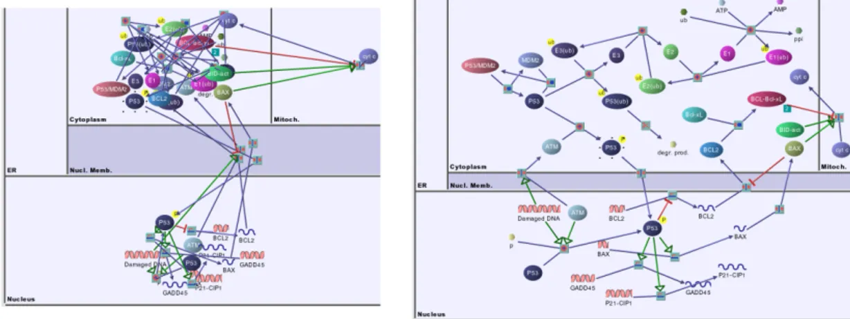
pro-teins biological network shown in Fig. 1.1, using VISIBIOweb [2] . 2 1.3 Random node positioning (left) and automatically laid out (right)
versions of a biological network that respects cell compartments. . 3 1.4 Systems Biology Graphical Notation (SBGN) reference card [3] . . 4 1.5 Result of an automated layout algorithm applied on a biological
process diagram . . . 6 1.6 Proper SBGN layout of the biological diagram shown in Fig. 1.5 . 6
2.1 Sample compound graph created randomly using Chisio graph ed-itor [4]. . . 8 2.2 IFN regulation, a gene regulatory network. . . 9 2.3 From left to right: complex between phosphorylated cyclin and
CDK2 forming the maturation promoting factor in yeast, a tetramer of complexes between globin and heme, and a complex between calcium-calmodulin kinase II and another complex, itself formed of calmodulin and calcium [5]. . . 10
LIST OF FIGURES xi
2.4 Reaction between ATP and fructose-6-phosphate to produce fructose-1,6-biphosphate, ADP and a proton [5]. . . 11 2.5 Illustration of a generic force-directed method: the graph
(top-left) represented as springs and particles (top-right), reached stable state (bottom-right), corresponding graph (bottom-left) [6]. . . 13 2.6 A sample compound graph (left) and its corresponding model in
CoSE (right) [7] . . . 15 2.7 Total area is divided into 3: A (rectangular objects), B (wasted
area) and C (additional wasted area if aspect ratio is specified as 2). 21 2.8 A sample disconnected graph layout given the aspect ratio, with
and without packing, respectively. . . 22 2.9 A sample result of tiling algorithm, where the numbering indicates
the order of processing. . . 24 2.10 Polyomino constructed from a simple graph (left) and its bounding
box (right). . . 24 2.11 Packing results of a arbitrarily shaped object set using two
meth-ods: tiling (left) and polyomino packing (right) [8]. . . 25 2.12 A simple polygon (left) with no obstacles and the visibility graph
edges (right) . . . 26 2.13 A set of objects (top), its horizontal visibility graph (bottom-left)
and vertical visibility graph (bottom-right), with no directions specified. . . 27
3.1 CoSE fails to separate substrate, production and effector nodes (left), desired result (right). . . 29
LIST OF FIGURES xii
3.2 A disconnected graph laid out using CoSE (top) and SBGN with tiling (bottom). Disconnected molecules are shown using red, where complexes are represented by octagonal boundaries. . . 32 3.3 Polyomino representation and the polyomino cells of two objects. 34 3.4 Polyomino packing result on a sample graph. . . 36 3.5 A dummy complex is created to group each disconnected molecules
at each depth (large margins for dummy complexes are used to get a better understanding). . . 38 3.6 Two sample dummy complexes that have non-zero degree child
nodes. . . 39 3.7 Vertical visibilities of a node set (top-left), vertical compaction
result (top-right), horizontal visibilities (bottom-right) and result of horizontal compaction (bottom-left). . . 42 3.8 Process node handling in CoSE (left), how SBGN defines it to be
(right) . . . 43 3.9 Illustration of a process node (orange) using dummy compound
(yellow), port nodes (green) and rigid edges (red) in SBGN-PD layout. . . 43 3.10 Rotational force acting on a sample process node. . . 46 3.11 A sample layout, where net rotational force fails to detect 90-degree
rotation. . . 47 3.12 Reference card for rotational force signs for four possible
orienta-tions: left-to-right, right-to-left, top-to-bottom, and bottom-to-top. 48
4.1 Comparison of tiling, polyomino packing without compaction and polyomino packing with compaction . . . 51
LIST OF FIGURES xiii
4.2 Percentage of properly oriented edge count to total number of edges
to be oriented with different value sets. . . 53
4.3 Effect of approximation distance on results. . . 54
4.4 Effect of rotation period on results. . . 55
4.5 Effect of angle tolerance on results. . . 55
4.6 Effect of 90-degree rotation constant on results. . . 56
4.7 Effect of 180-degree rotation constant on results. . . 57
4.8 Effect of approximation period on results. . . 57
4.9 Effect of phase 1 maximum iteration count on results. . . 58
4.10 Comparison of CoSE and SBGN-PD average results. . . 58
4.11 Comparison of CoSE and SBGN-PD average execution times. . . 59
4.12 Effect of (N+E) on the average result for non-compound graphs. . 60
4.13 Effect of (N+E) on average execution time for non-compound graphs. 60 4.14 Effect of (N+E) on the average result for compound graphs. . . . 61
4.15 Effect of total number of nodes and edges on the average execution time for compound graphs. . . 62
4.16 Comparison of polyomino packing (left) and tiling (right). . . 63
4.17 Btg family proteins and cell cycle regulation network laid out using SBGN-PD. . . 64
4.18 Vitamins B6 activation to pyridoxal phosphate network laid out using SBGN-PD. . . 65
LIST OF FIGURES xiv
4.20 5HT1 type receptor mediated signalling pathway laid out using SBGN-PD. . . 67 4.21 Aspirin blocks signalling pathway involved in platelet activation
laid out using SBGN-PD. . . 68 4.22 Process between ATM and RBBP8 laid out using SBGN-PD. . . . 69 4.23 Carm1 and regulation of the estrogen receptor pathway laid out
using SBGN-PD. . . 70 4.24 Tie2 signaling pathway laid out using SBGN-PD. . . 71
Chapter 1
Introduction
1.1
Motivation
One of the most famous idioms states that: “A picture is worth a thousand words”. That phrase lays the foundation of information visualization. Fig. 1.1 and Fig. 1.2 illustrate the fact that it is easier to interpret data in visual format. Since the beginning of mankind, visualization has been effectively used. Even the ancient people were drawing hieroglyphs and diagrams on the cave walls to express themselves. It is stated that, the diagrams directly address people’s innate cognitive abilities [9]. Due to the fact that symbols, diagrams and other graphical representations spread all over the world, it is necessary to have a common interpretation. Therefore, standard notations play an important role in communication and rapid development of many research areas. For instance, in the field of electronics, people use a common circuit design notation, which fastens the development and research quality.
Going back a few years ago, biologists did not have a common language for representation of their research results [10]. Studies included intensive usage of graphical elements but there were poor similarities between them when compared. There were no standard notation to visualize biochemical reaction pathways, signal transduction on the cell surface or inside the cell and genome regulation
Figure 1.1: “ATM mediated phosphorylation of repair proteins” biological net-work shown in Pathway Commons [1]
Figure 1.2: Visualized version of ATM mediated phosphorylation of repair pro-teins biological network shown in Fig. 1.1, using VISIBIOweb [2]
diagrams. Already present notations were fulfilling the needs of some groups of researcher but when used by others, resulting in ambiguity [11].
In 2005, a group of modellers, biochemists and software engineers have started working on a standard notation and in 2009, they published the Systems Biol-ogy Graphical Notation (SBGN) [?]. This notation allows scientists to represent biological pathways and networks in an easy-to-understand and efficient way. It consists of three complementary languages: process descriptions (PD), activity flows (AF) and entity relationships (ER).
In the last years, scientist have developed some other non-graphical notations for representing biological network information [12] and in the meantime over 300 biological network and protein interaction databases have been formed [13].
As intended, SBGN attracted considerable attention of the scientists and many software supporting this notation have been developed [14]. A person can create a new pathway or load a previously created one from listed databases using those tools. The tools also allow automated layout of those networks. This feature is crucial because, a nicely laid out graph helps the user to understand the underlying data faster, whereas a bad drawing may be misleading and confusing as can be seen in Fig. 1.3.
Figure 1.3: Random node positioning (left) and automatically laid out (right) versions of a biological network that respects cell compartments.
Figure 1.4: Systems Biology Graphical Notation (SBGN) reference card [3]
Until recently, most of the studies about automated layout have been focused on visualization of biochemical pathways. There are many software tools support-ing SBGN and many studies on layout of biological networks [15] [16] [17] [18] [19]. However, none of them are specializing in automatic layout of SBGN process di-agrams.
Process descriptions are intended to show change. A process description map represents processes that transform physical entities into other entities as a result of different influences [11].
The main purpose of this research is to represent process description maps in SBGN as clear and understandable as possible. We aim to speed up the compre-hension and analysis steps of biological pathways for scientists by supporting the SBGN standard notation.
1.2
Contribution
We propose a new automated layout algorithm that enforces SBGN-specific rules. Those rules include separating different reactions by using associated compart-ments, tiling of zero degree members and proper orientation of processes and their neighbors.
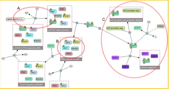
The sample biological diagram in Fig. 1.5 is laid out using a general purpose layout algorithm. The tool [20] supports SBGN by drawing nodes and edges properly. However, that layout exhibits three problems that we address to solve in our proposed layout algorithm.
First problem is that, SBGN states that product and substrate edges of a process node (represented as small gray squares) should be placed on opposite sides of associated process nodes (A). Moreover, each process node should have two port nodes: an input and an output port. The products of a process should be connected to the output port and substrates should be connected to the input port. Secondly, the classical layout does not tile degree zero members inside the
complexes (represented as rectangles with information bulbs) (B). Lastly, the reactions that occurs inside the nucleus is not separated from the other reactions occuring in other places (C).
In this thesis, we propose a new layout algorithm to we obtain a more proper and compliant SBGN process description diagram (Fig. 1.6).
Figure 1.5: Result of an automated layout algorithm applied on a biological process diagram
Chapter 2
Background and Related Work
2.1
Graphs
A graph is a representation of a set of discrete objects and their relations. The objects are called nodes or vertices and the links are called as edges. Mathematical notation of a graph is G = (V, E), where vertex v ∈ V and edge e ∈ E. An edge e represents a connection between two nodes and is represented by e = (u, v), where u, v ∈ V . If two vertices u and v are connected to each other by an edge e, those two vertices u and v are said to be adjacent vertices and they are incident to e.
A graph may have a directed or undirected structure. If pairs (u, v) are or-dered, the graph is said to be a directed graph. In that case, in-degree of a node v is calculated as the total number of incident edges that have their target nodes as v and out-degree is the total number of incident edges where their source nodes are v, respectively. Undirected graph vertices do not have a specific in/out-degree. In both cases, degree of a node is the total number of incident edges of that node. A graph may have child graphs. In that case, if G = (E, V ), Gi = (Ei, Vi)
and Gi ∈ V and similarly, parent of Gi is G. A node that have children nodes
of the root is referred as root graph.
A compound graph can be identified as having a number of edges that connect two nodes, whose parents are different from each other. It is shown as C = (V, E, F ) where V stands for vertex set, E for edge set and F is the inclusion edge set. Inclusion graph T = (V, F ) is an inclusion tree. T does not include any edges connecting a node to its children or parent nodes. Fig. 2.1 illustrates a compound graph, where blue nodes represent simple nodes, which do not have any children and conversely red labelled nodes are compound nodes, which have child graphs. For instance, 4 is a compound node, which has 1 as its parent node, which, in turn, is a compound node with children 8, 9, 31, 33, 38, 39.
Figure 2.1: Sample compound graph created randomly using Chisio graph editor [4].
One common data structure to implement a compound graph is a graph man-ager, which stores the nested structure of compound graphs. A graph manager M = (S, I, F ) is defined by a set of inter-graph edges I, a set of compound graphs S = G1, G2, ..., Gn and a rooted nesting tree F = (VF, EF) [7]. Each node may
have different sizes. If a node is a compound node (i.e., it has a child graph), its bounding box is calculated with respect to the bounds of its child graph in a nested manner.
2.2
Systems Biology Graphical Notation
The Systems Biology Graphical Notation (SBGN) is a standardized visual repre-sentation of biochemical cellular processes. It is developed by a group of software engineers, modellers and biochemists. It defines some sets of symbols and rules by defining their usage. Fig. 2.2 ilustrates a sample SBGN process description map.
Figure 2.2: IFN regulation, a gene regulatory network.
In the recent years, many software tools have been developed for pathway and network design such as PATIKA, CellDesigner, NetBuilder [21] [22] [23]. However all those tools have used their own notations. Therefore, representation of a network resulted in different visuals, causing ambiguity and slowing down the research process. This problem raised the need to have a standard notation and triggered SBGN to be formed.
An SBGN Process Description map is fundamentally a bipartite graph, i.e., its vertices can be divided into two disjoint sets such that each vertex in one set connects to a vertex in the other set, with no edges allowed between two nodes in the same set. One of those sets corresponds to process nodes and the other one to entity pool nodes. Another structure is compartments, which may contain some entity pool nodes. The entities are referred to as glyphs and the edges as arcs.
There are six glyph classes in entity pool nodes: unspecified entity, simple chemical, macromolecule, nucleic acid feature, and complex. Those materials may contain extra information such as state variables, units of information and clone markers (Fig. 1.4).
Figure 2.3: From left to right: complex between phosphorylated cyclin and CDK2 forming the maturation promoting factor in yeast, a tetramer of complexes be-tween globin and heme, and a complex bebe-tween calcium-calmodulin kinase II and another complex, itself formed of calmodulin and calcium [5].
For the layout process, one of our main concern are complexes. A complex node represents a biochemical entity, which is composed of some other biochem-ical entities. A complex is represented by a node that have octagonal bound-aries. Children of complexes do not have edges to other entities. Hence, they
are disconnected nodes. The rule for complex member placement is to tile those disconnected members. Fig. 2.3 illustrates a number of complexes in SBGN.
Another important concern for us is the process nodes. A process node repre-sents processes that transform a number of entity pools into a number of another entity pools. The generic rule for the process nodes is that, they have two port nodes. One of them is for substrates (input) and the other one is for products (output). SBGN specifies that the port nodes should be placed on the opposite sides of its corresponding process node. Fig. 2.4 illustrates a process node with two inputs (left) and three outputs (right).
Figure 2.4: Reaction between ATP and 6-phosphate to produce fructose-1,6-biphosphate, ADP and a proton [5].
2.3
Automated Layout
Information visualization plays a crucial role to improve understanding of people on a given data set. After data has been queried from databases and its irrelevant parts have been filtered out, it is ready to be visualized for analysis.
There has been lots of research on graph layout [24] [25]. The purpose of performing layout on a graph is to make visualization as clear and pleasant to the eye as possible. Because a poor layout of a graph may confuse the user’s mind, whereas a good, aesthetically pleasing layout helps with understanding the data easily (Fig. 1.5 and Fig. 1.6). Criteria of a good layout may differ from person to person. However, the following are some generally accepted ones [24]:
• Minimize total drawing area
• Minimize number of edge-edge crossings • Minimize total edge length
• Support uniform edge length • Reflect the symmetry of the graph
In addition to those items, for our case, considering the fact that biological pathways include nested diagrams, it is important to use a layout algorithm that respects the nested structure. In other words, one of our criteria is to find an automated layout algorithm that places a child node of a compound node such that the boundaries of the compound node completely contains the boundaries of the child node plus user-defined margins.
Force-directed layout algorithms (also known as spring embedders) is proba-bly the most popular approach for automatic layout of graphs. In 1984, Eades used a novel modelling for a graph: he considered nodes as steel rings and edges as stretchable springs [26]. In this algorithm, each node applies repulsion force to all other nodes in the graph and attractive force to its adjacent nodes.
The following equation is used for calculating the repulsion force between two non-adjacent nodes u, v [6]:
frep(pu, pv) =
cr
kpv− puk2
· −−→pupv (2.1)
He uses his own formulations to calculate spring forces, instead of using the exact Hooke’s law formulations. If two nodes u and v are adjacent, which means that they have an edge connecting them to each other, the force acting between those two nodes is calculated using the edge, as follows:
fspring(pu, pv) = cs· log
kpv − puk2
Here, pu denotes the position vector of u, cr is the repulsion constant, csis the
spring constant to control spring strength and l is the length of the edge. The algorithm performs those calculations, until the total displacement of nodes falls under a predefined threshold, indicating that the system became stable (Fig. 2.5).
Figure 2.5: Illustration of a generic force-directed method: the graph (top-left) represented as springs and particles (top-right), reached stable state (bottom-right), corresponding graph (bottom-left) [6].
Kamada and Kawai enhanced Eades’ algorithm by introducing the desirable (Euclidean) distance concept, using graph theoretic distance [27]. By doing so, they calculate attractive forces between not only adjacent nodes, but also nodes that are not adjacent but within an ideal distance. They also worked on minimiz-ing the total sprminimiz-ing energy of the system. As a result, their algorithm produced
successful results on drawing symmetric graphs and resulted in small number of edge crossings.
Later, Fruchterman and Reingold improved Eades’ algorithm and proposed an advanced version [28]. They have used the uniform edge length concept. Their algorithm has two main principles: if two nodes are adjacent, draw them close to each other, but do not draw any two nodes too close to each other. They use a formula similar to Hooke’s law formulations for spring force calculations. In Hooke’s law, force F is defined as F = −kx, where k is defined as spring constant and x is defined as the distance from spring’s current position to desired position. Although those algorithms perform well especially on small scaled graphs, they do not produce good results for the graphs that have a few hundred or more nodes. The main reason of this problem is that, layout process has many local minima. In order to skip local minima, simulated annealing’s cooling process has been imitated but Kobourov states that even more complex approaches do not guarantee to skip local minima [29].
2.4
Compound Spring Embedder
Compound Spring Embedder (CoSE) is a force-directed graph layout algorithm that aims to satisfy the generally accepted graph drawing criteria for compound graphs [7]. CoSE is based on Fruchterman and Reingold’s algorithm discussed in the previous section. Additionally, CoSE has support for inter graph edges, non-uniform node sizes and clustered graphs.
This automated layout algorithm treats the nodes as charged particles, edges as springs and it symbolizes each compound node as a “cart”. Therefore, a nested compound structure can be represented with multiple carts on top of each other, where a cart may contain a number of objects and other carts.
During the layout process, two nodes can repel or pull each other depending on the distance between them. If those nodes are adjacent, force calculation
depends on the tension of their edge. If they are not adjacent and located too close, they apply repulsion forces on each other, which is a similar approach to the one that Fruchterman and Reingold have proposed. Repulsion forces ensure avoiding overlaps between nodes as much as possible.
CoSE also uses gravitational forces. The aim of this force is to keep children of a node closer to the center of their parent, thereby by keeping the children nodes together. Similarly, in the case of the root graph, the gravitational forces keep disconnected graphs together. The results show that this force is useful for reducing the total drawing area.
To illustrate, in Fig 2.6, the nodes represented with filled rectangles in the sample graph are simple nodes, whereas the nodes with no fill are compounds. In the corresponding model, it is seen that all nodes are positively charged. There are gravitational force locations at the center of each compound node and at the center of the root graph. The distance between the gravitational force locations and the nodes affected by that point are shown using red lines.
Figure 2.6: A sample compound graph (left) and its corresponding model in CoSE (right) [7]
CoSE supports non-uniformly sized nodes. The algorithms that do not sup-port varying node sizes, can make use of uniform edge lengths. However, having different node sizes results in some difficulties such as adjusting the edge length. For instance, a predefined edge length may be shorter than the distance be-tween the centres of two nodes, if at least one of them has a big bounding box. Therefore, if non-uniform node sizes is supported, a specialized ideal edge length calculation should be provided. CoSE overcomes this problem by using clipping points. Clipping point of a node is defined as the intersection point between the edge, which is defined from center point of the source node to the center point of the target node, and the bounding box of the node. The ideal edge length is then defined as the length between two clipping points.
Because of the fact that there are varying node sizes, finding an ideal edge length, that is valid for all nodes is not possible. Thus, CoSE defines an ideal edge length for each edge, depending on the number of nesting structures it spans. In order to do that, lowest common ancestors of two end nodes are found first. Then, using the ancestors, clipping points of the nodes are calculated and the distance from nodes to the corresponding clipping points are added to the ideal edge length. After ideal edge lengths for all edges are found, initial positioning of the nodes are performed. If the user does not run incremental layout, initial positioning is performed randomly or radially, depending on the graph type, which in this case being flat and forest or not. The pseudo code of the initialization step can be found in Algorithm 1.
After the initialization step is completed, the forces (repulsion, spring and gravitational) are applied on nodes until the system reaches a steady state or a maximum iteration count. If the total displacement between two iterations is below some predefined threshold, the algorithm is said to be stable. The cooling scheme used by CoSE is a linearly decreasing function (Algorithm 2).
Algorithm 1 CoSE Initialization
1: function classicLayout()
2: calcLowestCommonAncestors()
3: calcInclusionTreeDepths()
4: calcIdealEdgeLengths()
5: if layoutT ype 6= incremental then
6: if graph is f orest and f lat then
7: positionNodesRadially() 8: else 9: positionNodesRandomly() 10: end if 11: end if 12: initSpringEmbedder() 13: runSpringEmbedder() 14: end function
Algorithm 2 Perform Layout
1: function runSpringEmbedder()
2: while totalIterations < maxIterations do
3: totalIterations ← totalIterations + 1 4: if isConverged() then 5: break 6: end if 7: updateBounds(graphManager) 8: calcSpringForces() 9: calcRepulsionForces() 10: calcGravitationalForces() 11: moveNodes() 12: end while 13: end function
2.4.1
CoSE Layout Structure
CoSE makes use of a graph manager that keeps track of all subgraphs, all edges (including inter-graph edges) and all nodes.
As discussed previously, CoSE calculates spring, repulsion and gravitational forces at each iteration and moves each node with respect to total force acting on it. SBGN-PD layout uses the existing forces of CoSE with some modifications. Therefore, in order to specify the modifications, we explain the methods in detail. Spring forces are calculated for each edge in CoSE. This method first updates the edge length using the end nodes centres, as opposed to clipping points to simplify calculations involved or using the rectangles representing the geometry of the nodes. Then, the spring force is calculated and applied on the end nodes. Algorithm 3 Calculate Spring Forces
1: function calcSpringForces() 2: for all e = (u, v) ∈ E do
3: edge ←updateLength(edge)
4: springF orce ← cs∗ (edge.length − idealLength)
5: u.Fspring~ ← u.Fspring~ + springF orce
6: v.Fspring~ ← v.Fspring~ − springF orce
7: end for
8: end function
Repulsion forces are calculated for each pair of nodes that are either adjacent nodes or within some distance. In order to find if two nodes are within some distance, CoSE uses either grid variant structure proposed by Fruchterman and Reingold or simply checks for the distance between each node. It is important to note that the repulsion force calculations for each node is different for those two cases:
• If FR grid variant is active, the surrounding nodes of the given node are detected first and then the repulsion force is applied if both of them are in the same graph.
Algorithm 4 Calculate Repulsion Forces
1: function calcRepulsionForces()
2: if type is useF RGridV ariant then
3: grid ←calculateGrid() 4: for all v ∈ V do 5: addNodeToGrid(v) 6: end for 7: for all v ∈ V do 8: calculateRepulsionForceOfANode(v, grid) 9: end for 10: else 11: S := {} 12: for all v ∈ V do 13: S := S ∪ {v} 14: for all u ∈ V − S do 15: calcRepulsionForce(u, v) 16: end for 17: end for 18: end if 19: end function
two nodes overlap, repulsion force is calculated using the overlap amount. If they do not overlap, the distance between them is updated according to the clipping points and force is calculated using the updated distance.
Gravitational forces keep the components of a graph as close as possible. If the graph is a disconnected graph and gravitational forces are not used, discon-nected components may be placed far from each other, yielding in arbitrarily huge drawing areas. In order to minimize the total drawing area and keep the components close to each other as much as possible, children nodes of graphs are attracted towards the center point of the bounding rectangles of them.
During the calculation of gravitational forces, this force is applied on a node only if the node is “roughly” outside the bounds of the initial estimate for the bounding rectangle of the owner graph. Gravity range factor gf, gravity constant
cg, compound gravity range factor gcf and compound gravity constant cgc are
constants to relax the estimated sizes of the owner graphs because their bounding boxes are tight. Estimated bounding box of the root graph is relaxed more, when
compared to relaxation of a compound node. Algorithm 5 Calculate Gravitation Forces
1: function calcGravitationForces()
2: for all v ∈ V do
3: o ← v.ownerGraph
4: distance ← v.center − o.center
5: if (o is rootGraph) ∧ (|distance| ≥ o.estSize ∗ gf) then
6: v. ~Fgrav = v. ~Fgrav− distance ∗ cg
7: else if (o is compound) ∧ (|distance| ≥ o.estSize ∗ gcf) then
8: v. ~Fgrav = v. ~Fgrav− distance ∗ cg∗ cgc
9: end if
10: end for
11: end function
After all the forces are calculated, each node is moved with respect to the net force acting on it, where ~Fnet = ~Frep+Fspring~ +Fgrav~ . In this location translating
process, if a node is a compound node, the forces acting on the compound is propagated to its children. As a result, not only the compound node, but also the locations of its children are updated.
Algorithm 6 Propagate Displacement To Children
1: function propagateDisplacement(v, ~Fdisp)
2: for all u ∈ v.childGraph do
3: u.center ← u.center + ~Fdisp
4: if u is compound then 5: propagateDisplacement(u, ~Fdisp) 6: end if 7: end for 8: updateBounds(v.childGraph) 9: end function
Considering the fact that, attractive forces are calculated for each edge (|E|), repulsive forces are calculated for each vertex pair (|V |2) and gravitational forces are calculated for each vertex (|V |), CoSE is resulting in a per iteration complexity of O(|E| + |V |2).
2.5
Rectangle Packing
Most of the graph drawing algorithms try to minimize drawing area by assuming that the graph is connected [30]. This minimization is achieved by finding the bounding box of a graph, or in other words, finding the smallest rectangle that the graph can fit in. However, if the graphs have disconnected members and the layout algorithm is poor, resulting layout may contain large wasted area. Additionally, if user specifies an aspect ratio, which is defined as the ratio between resulting container’s width and height, then the packing result should respect the desired ratio and the result may contain even more wasted area (Fig. 2.7).
A B
C h
w = 2h
Figure 2.7: Total area is divided into 3: A (rectangular objects), B (wasted area) and C (additional wasted area if aspect ratio is specified as 2).
Rectangle packing problem can be defined as packing a number of non-uniformly sized, rectangle shaped objects into a container such that there will be no overlaps between the objects and the container will be as compact as possi-ble. More formally, given a set of n rectangular items i ∈ S1,...,n, each defined by
a width wi and hi, find the container R that covers each item i and the wasted
area is minimum. This problem, defined in two-dimensions, is an NP-hard prob-lem [31].
Fig. 2.8 illustrates the affect of packing on wasted area. The sample graph has two disconnected graphs and each of those graphs have 10 nodes. The layout algorithm is given an aspect ratio. It is seen that properly tiling disconnected components gives more aesthetically pleasing results with less wasted area.
a b c d e f g h i j k l m n o p r s t u a b c d e f g h i j k l m n o p r s t u
Figure 2.8: A sample disconnected graph layout given the aspect ratio, with and without packing, respectively.
Fullness of a drawing is calculated as the total area covered by the objects divided by the total drawing area. It is denoted by F (L). Adjusted fullness, on the other hand, expresses the fullness of a drawing, when the aspect ratio is being used. It is denoted by AF (L). For Fig. 2.7:
F (L) = A
A + B (2.3)
AF (L) = A
A + B + C (2.4)
Aspect ratio performance(ARP) of a packing algorithm can be calculated as follows:
ARP (L) = min(AR(L), DAR(L))
where L denotes the list of objects, AR(L) is the aspect ratio produced by the algorithm and DAR(L) is the desired aspect ratio.
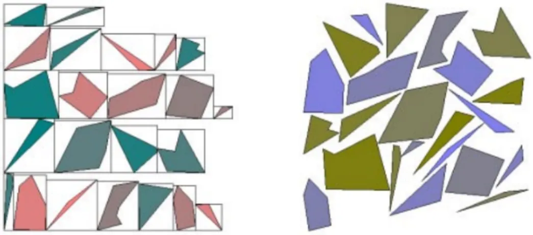
There are a number of different methodologies for rectangle packing such as bin packing, strip packing, alternate-bisection method, tiling and polyomino packing [30] [32] [8]. Below we examine two of those algorithms, which are tiling and polyomino packing. Tiling method gives good results in adjusted fullness and respects the aspect ratio [30]. On the other hand, polyomino packing supports not only rectangle shapes but also arbitrarily shaped objects.
2.5.1
Tiling
The general view to the tiling algorithm is that: the resulting container is com-posed of a number of strips, that are placed on top of each other. A strip is a horizontal container, that stores a number of objects. Therefore, tiling is defined as a type of strip packing problem. In strip packing, the strip is given with a fixed width value, which is calculated using the desired aspect ratio. However, tiling uses a strip, whose width changes dynamically.
The algorithm first, sorts the objects in descending order of their width sizes. Then, the first level strip is created and the first object is placed in it. Its width becomes equal to the width of that object. One by one, all objects are placed into the container by deciding whether to place the next object into the shortest strip or create a new strip. The condition for an object to be placed into the shortest strip is having enough space.
Fig. 2.9 shows a sample result of the algorithm. The experiments show that if the objects are not sorted in increasing order of their heights, the results become more compact [30]. The algorithm takes O(n lg n) time and has serious advantages in terms of adjusted fullness and aspect ratio performance over its competitive types.
1
2
7
9 10 113
4
56
8
12
13
14
15
Figure 2.9: A sample result of tiling algorithm, where the numbering indicates the order of processing.
2.5.2
Polyomino Packing
A polyomino is a geometric figure formed by joining unit squares at the edges [8]. A polyomino represents a graph object. Thus, if the graph is a disconnected graph, each disconnected component is represented using a polyomino. Fig. 2.10 illustrates a sample polyomino of a graph.
Figure 2.10: Polyomino constructed from a simple graph (left) and its bounding box (right).
The polyomino packing algorithm uses a greedy heuristic. Initially, the poly-ominoes of the objects are created. Then, a finite grid, that can cover all polyomi-noes fully or partially, is constructed. After the initialization is completed, each
polyomino is inserted into the grid one by one. The optimal place of a polyomino is where cost function max(|x|, |y|) is minimum. In order to find the optimal place, each empty cell is sequentially scanned in the increasing order of the cost function. This means that the cells near to the already placed polyominoes are checked first. If the polyomino fits in a position without causing any overlaps, the corresponding polyomino cells are marked as full.
It is very crucial to set a good grid cell size s. Because, increasing the cell size means increasing the wasted area, whereas using a small grid size increases the running time of the algorithm by almost checking each point in the grid. The quadratic equation below can be used to calculate l, where c is some constant, s is the average polyomino size and s ≤ c.
(cn − 1)l2− n X i=1 (Wi+ Hi)l − n X i=1 WiHi = 0 (2.6)
For the analysis, the algorithm scans each grid cell to find a suitable grid for each polyomino. When an empty grid cell is found, each neighboring cells corresponding to polyomino cells are checked to see if the polyomino fits into that empty grid cell. Therefore, the algorithm takes O(n2s2) but since s is a
constant, the algorithm is of O(n2), where n is the number of objects to be
packed. Fig. 2.11 shows a comparison of polyomino packing and tiling layouts.
Figure 2.11: Packing results of a arbitrarily shaped object set using two methods: tiling (left) and polyomino packing (right) [8].
Considering that, a grid cell size may not have been properly set. As indicated previously, large grid cells result in large wasted area. In order to reduce that wasted area, a compaction may be performed on the resulting layout as post-processing.
2.6
Compaction
Compaction process is used to obtain more compact results from the tiled graphs. If the objects are drawn more compact, it may decrease the wasted area and result in smaller bounding box, which is a requirement for obtaining more aesthetically pleasing drawings.
Visibility graphs may be used to perform compaction. Visibility graphs are commonly used for planning robot paths. For instance, Nilsson described a system for planning the motion of robotic systems among obstacles in 1969 [33] [34]. He introduced the visibility graph and combined it with A* heuristic to find the shortest, collision-free path amidst obstacles between the robot’s location and the destination point.
A visibility graph is described as Gv = (Ev, Vv) and it indicates the visibility
relation between a set of nodes. The visibility refers to the feasibility of drawing a collision-free straight line between two nodes (Fig. 2.12).
Figure 2.12: A simple polygon (left) with no obstacles and the visibility graph edges (right)
In this context, nodes are defined as point locations and edges are visible connections. However, for the simplicity of the problem, we use the set of objects as the set of nodes instead of using point locations.
There has been intensive research on visibility graphs in 1980’s [35] [36] [37] [38]. The naive approach runs in O(n3) and the studies show that it can be improved to O(n2) by using sweep lines.
The visibility graphs can be applied to a number of shapes such as convex polygons, line segments and simple polygons. An illustration of visibility graph on rectangular objects can be found in Fig. 2.13. We are interested in only the vertical and horizontal visibilities.
A
B
C
E
D
F
G
H
B
A
C
D
E
G
H
F
D
A
F
E
B
G
C
H
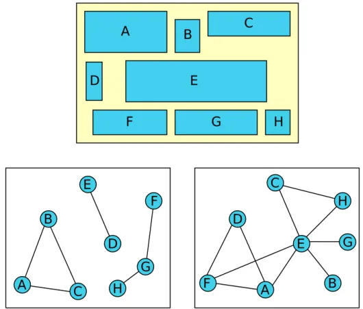
Figure 2.13: A set of objects (top), its horizontal visibility graph (bottom-left) and vertical visibility graph (bottom-right), with no directions specified.
Chapter 3
SBGN-PD Layout
SBGN-PD layout is a specialized automated layout algorithm for SGBN process description maps. It uses the force-directed CoSE layout algorithm as basis. Sat-isfying SBGN rules brings additional constraints to this layout problem. On top of the CoSE structure, we add a new type of force and associated procedures. In the following sections, enhancements to the original CoSE algorithm and adaptation of previously discussed algorithms are going to be explained in detail.
Spring force and repulsion force calculations are modified by SBGN-PD layout to prevent wrong relocation of process and port nodes (see section 3.2 for details). Additionally, a new force called as rotational force is introduced.
CoSE has only one phase for performing layout (see Algorithm 2), whereas SBGN-PD layout uses a two-phase algorithm. The first phase is almost identical to CoSE procedure, except it has a relatively small, fixed number of maximum iterations and it uses the modified force calculation methods.
In the second phase, the maximum number of iterations is initially calculated by taking the logarithm of total number of node and edges. Logarithm function ensures a slow growth. The reason behind using this calculation is to have less maximum number of iterations for small graphs in the second phase, whereas more iterations may be needed for a more complex graph.
Algorithm 7 Second Phase of SBGN-PD Layout
1: function doPhase2(G)
2: maxIterations ← log(GV.size + GE.size) ∗ c0
3: initialCoolingF ac ← ccool
4: while totalIterations < maxIterations do
5: totalIterations ← totalIterations + 1
6: if approximationP eriod is reached then
7: approximateLocations()
8: end if
9: if isConverged() and areEdgesProperlyOriented() then
10: break 11: end if 12: updateBounds(graphManager) 13: calcSpringForces() 14: calcRepulsionForces() 15: calcGravitationalForces() 16: moveNodes() 17: end while 18: end function I1 I2 O1 O2 Eff P O3 I1 I2 O1 O2 Eff P O3
Figure 3.1: CoSE fails to separate substrate, production and effector nodes (left), desired result (right).
Additionally, in the second phase, the cooling factor starts from a smaller value to not to alter the result of first phase. However, this brings along some problems such as not being able to place substrate and production nodes close to each other or put the effector node in between those (Fig. 3.1). Because, CoSE does not respect the node types, it only considers the shapes and their overlap amounts. Therefore, in addition to those modifications, this phase applies a location approximation algorithm for product and substrate nodes and another one for effector nodes at certain iterations.
The approximations are only applied a few times. Product and substrate node approximation is performed to prevent two nodes that connect to different port nodes getting stuck on the reverse sides. Because of the fact that placement of nodes at the end of the first phase does not respect port node locations, the approximation is needed. In addition to this, cooling factor is decreased to a small value to prevent alteration. However, decreasing the cooling factor also prevents, for instance a product node to jump over a substrate node and get located near its own port node.
Although we want all nodes to be close to their own port nodes, the algorithm should not interfere much with a highly connected node. Because, for these types of nodes, forcing their locations to another point may cause long edges and poor layout. Therefore, we only apply approximation for degree-one nodes.
The calculation is done as follows: find all port nodes and their production or substrate nodes. Group multi-edge nodes and degree-one nodes separately. After that, for each group, find an approximation point using the locations of multi-edge nodes. On the other hand, if a port node has only degree-one nodes, then one of those nodes is selected randomly for the approximation point. At the end, all degree-one nodes are moved within a circle, whose center point is the approximation point and radius is a constant.
Location approximation for effector nodes is performed similarly. An effector node may get stuck between some production or substrate nodes. In order to prevent this, all effector nodes of a process node are found and grouped separately. Then, location of each effector node is changed with respect to the orientation of
the associated process node. Location of the effector node is always approximated within an ideal edge length distance from process nodes’ center. There are four cases to consider: process node is oriented vertically and effector should be placed on its left or right, or the process is oriented horizontally and effectors should be placed on its top or bottom.
For instance, illustration of a vertical-left scenario works as follows: if port nodes of a process node is placed vertically, its effector nodes should be placed either on its left or right. If an effector is already placed on the left of the process node, calculate a target point from process node to ideal edge length distance to the left and place the effector node within an circle close to the approximation point. The other cases are handled similar to this one.
As mentioned previously, SBGN-PD layout introduces rotational forces. A rotational force is calculated at each step and it is applied while moving the nodes. This force is discussed in detail in section 3.3.
3.1
Nested Rectangle Packing
In order to achieve compact and proper drawings of SBGN process maps, dis-connected nodes must be packed. A disdis-connected node may either be a member of a complex node or a degree-zero molecule that is not owned by a complex. A graph may need rectangle packing for two reasons:
• Tiling of complex members: Tiling of complex members is required by SBGN. It is important to note that, a complex node may have another complex node as its child. Therefore, the problem becomes a nested rect-angle packing problem.
• Tiling of disconnected molecules: Disconnected graphs may result in large wasted area. In order to reduce it, we perform packing for all disconnected molecules at each level, that are not owned by any complex nodes. In the rest of the document, a disconnected molecule refers to a degree zero node,
whose owner is not a complex, for convenience.
Fig. 3.2 illustrates layout of a sample disconnected graph. CoSE does not perform packing and results in a huge wasted area when compared to SBGN-PD (Fig. 3.2). complex1 complex2 A B C D G F E A B C D E F G complex1 complex2
Figure 3.2: A disconnected graph laid out using CoSE (top) and SBGN with tiling (bottom). Disconnected molecules are shown using red, where complexes are represented by octagonal boundaries.
In order to handle the nested structure, a recursive approach is needed. In this recursive algorithm, processing order of complexes plays the key role. The processing should be performed in a bottom-up manner. Because, each time, bounding box of a complex is calculated using its child nodes. For instance, let v ∈ VG be a complex node and its depth vdepth = d, where d > 1 and
rootdepth = 0. In order to correctly tile the nodes at depth d − 1, vwidth and vheight
tiling complex members at depth d − 1, vwidth and vheight are going to be wrong.
Because, their values are going to be as their initial values. Hence, tiling at depth d − 1 is not going to be correct.
To achieve this bottom-up processing, depth-first search is performed on com-plex nodes of the graph. After finding all the comcom-plex nodes, rectangle packing is performed on each complex with respect to their orders.
Algorithm 8 Perform Layout
1: function layout()
2: groupDisconnectedMolecules()
3: complexOrder ←applyDFSOnComplexes()
4: for all complex ∈ complexOrder do
5: clearComplex()
6: end for
7: performLayout()
8: for all complex ∈ complexOrder do
9: repopulateComplex()
10: end for
11: end function
3.1.1
Packing Complex Members
A user can specify tiling or polyomino packing method to pack the complex members.
Tiling is a straightforward but elegant method that makes use of a container for the objects [30]. The container is composed of strips that are put on top of each other. After sorting each node with respect to their areas in decreasing order, they are inserted into the container one by one.
Aspect ratio is taken into consideration while making the decision about whether to place the object horizontally or vertically by creating a new strip. This decision is made by checking if width of the container increases in case of placing an object into the shortest strip. If it has no effect on the width, the object can be inserted horizontally. However, if the width increases, it may be
Algorithm 9 Tiling pseudocode derived from [20]
1: function insertNode(container, node) 2: if container if empty then
3: insertNodeToRow(container, node, 0)
4: else if canAddHorizontal(container, node) then
5: insertNodeToRow(container, node, container.shortestRowIndex)
6: else
7: insertNodeToRow(container, node, container.lastStripIndex + 1)
8: end if
9: end function
a good idea to place the object vertically. In this case, a new strip is created with that object. When a new strip is created, the container may get smaller by shifting the last element of the longest strip to the end of the new strip. There-fore, after each strip is created, a recursive check is performed to detect potential shifting operations.
Polyomino packing uses a grid structure and places the polyominoes on the empty grid cells [8]. Each polyomino consists of a number of polyomino cells. For instance Fig. 3.3 illustrates example of some sample polyominoes and their polyomino cells. Note that, if cell size is chosen carefully, a polyomino may result in less area when compared to the object’s bounding box.
Figure 3.3: Polyomino representation and the polyomino cells of two objects. In order to have a good cell size, a dynamical computation may be performed or a constant may be used. We use a predefined constant cl and adjust the value
step = 2
1 + aspectRatio (3.1)
cellSizeY = cl∗ aspectRatio ∗ step (3.2)
cellSizeX = cellSizeX ∗ step (3.3)
After the polyomino cell sizes are calculated, polyomino cells are created. When the cells are created, a random permutation of them are performed and their bounding rectangles are calculated. Then, a grid is created and polyominoes are inserted to the grid one by one.
Algorithm 10 Polyomino Packing Body
1: function pack(polyominoes)
2: makeGrid(dim, 0)
3: sortInIncreasingSize(polyominoes)
4: for all pmino ∈ polyominoes do
5: putMino(pmino)
6: end for
7: end function
The grid structure is initialized as a small grid first. Since its dimension (dim) may be too small to store all polyominoes, extra cells may be needed at any time. In order to achieve this, an enlargement step is applied. If extra cells are needed, grid is enlarged by some constant cenlarge and already placed polyominoes are
placed in the enlarged grid without losing their relative locations, before the new placement occurs.
In order to place a polyomino in grid, first, an unoccupied grid cell must be found. The check starts from center point of the grid and continues by increasing distance from center. A polyomino fits in a location only if all the grid cells corresponding to polyomino cells are unoccupied.
Fig. 3.4 illustrates the result of polyomino packing on a sample graph. In the sample graph, A, B and C are complexes. Members at different depths are coloured differently for convenience.
Algorithm 11 Placing A Polyomino Into Grid
1: function putMino(pmino)
2: while !tryPlacing(pmino) do
3: dim ← dim + cenlarge
4: makeGrid(dim, currentMinoes)
5: end while
6: for all cell ∈ pmino do
7: x =← cell.x + pmino.x 8: y =← cell.y + pmino.y 9: grid[x][y] ← occupied 10: end for 11: end function A0 A1 A2 B0 B1 B2 A B D E G F H I J A3 C
Initially, members of A and B are polyomino packed. Considering that all members of B have the same area size, one of them, which is B1 in this case, is
placed in the center and the other members B0 and B2 are placed around it.
Similarly, in order to pack the members of complex A, its members are sorted in decreasing order of their areas as A1, A0, A2 and A3. Then, A1 is placed in
the center, A0 and A2 are placed around it. In order to place A3, an unoccupied
cell is found, where the aspect ratio of A becomes as close as possible to desired aspect ratio. Finally, members of J are sorted as A, B, C, G, F , H, D, E, I and packed respectively.
3.1.2
Packing Non-Complex Members
CoSE uses gravitational forces to keep vertices close to the center as much as possible, but it may still not be sufficient to minimize the drawing area. There-fore, packing is performed on disconnected molecules to reduce the wasted area (Fig 3.2).
Considering that our layout algorithm supports complex member tiling, we make use of dummy complexes to pack disconnected molecules. This is achieved by grouping all disconnected molecules separately at each depth and assigning a dummy complex parent to them. This grouping should be performed at the very beginning of layout.
Fig. 3.5 illustrates tiling of non-complex members. In this figure, graph G is disconnected. C1 and C2 are two compound nodes, Cp is a complex node,
Z1, . . . , Z8, A and B are simple nodes. In this graph, none of the nodes are
connected to another node by an edge. Therefore, degrees of each node are 0. The graph manager stores 4 graphs, whose parent nodes are: root, C1, C2 and
Cp.
Cp is the parent of A and B and its type is complex. Therefore, although A
and B have no edges, considering that they have a complex parent, we do not refer them as “disconnected molecules”. Hence, a dummy complex is created at
C1 C2 Cp A B C1 D1 D2 Z1 Z1 Z2 Z2 Z3 Z3 Z4 Z4 Z5 Z5 Z6 Z7 Z8 C1 Z1 Z2 Z3 Z4 Z5 Z6 Z7 Z8 A B C2 Cp C2 D3 Z6 Z7 Z8 A B Cp
Figure 3.5: A dummy complex is created to group each disconnected molecules at each depth (large margins for dummy complexes are used to get a better understanding).
each level for each node group, except A and B. In this case, 3 dummy complexes are created:
• D1 is created at the root level (depth = 0), stores C1 and Z1
• D2 is created where depth = 1, stores C2, Z2, Z3, Z4 and Z5.
• D3 is created where depth = 2, stores Cp, Z6, Z7 and Z8.
The algorithm packs the members of all complexes in the following order: Cp, D3, D2 and D1. When members of a complex node is cleared out, its child
graph is removed from the graph manager. Then, layout is performed with the remaining nodes. After layout is done, previously cleared children of complexes are reinserted into the graph manager. In the final phase, the dummy complexes are removed from the graph. Although the algorithm seems straightforward, there are some important cases to handle.
A B D C E G F H I C1 C2 DC1 DC2
Figure 3.6: Two sample dummy complexes that have non-zero degree child nodes. Fig. 3.6 illustrates the fact that, using node degrees for compound nodes is misleading. Therefore, for each compound node v ∈ V , we define a graph degree GD(v) = y, where y is the total number of edges of all child nodes of v. For example, GD(C1) = 1 because of the edge between B and D. Similarly,
GD(C2) = 3 . On the other hand, node degrees of C1 and C2 are 0.
If node degrees were used instead of the graph degrees, members of C1 and
forces would not be calculated and after repopulation, A, B, E, F and G would be placed incorrectly. To overcome this problem, if a compound node is encountered while identifying the disconnected molecules, its graph degree value should be used to get a properly tiled result.
Algorithm 12 Graph Degree Calculation of a Compound Node
1: function calcGraphDegree(node)
2: degree ← 0
3: if node has no child then
4: degree ← nodedegree return degree
5: end if
6: for all child ∈ node.childGraph do
7: degree ← degree + nodedegree+ calcGraphDegree(child)
8: end for
9: end function
3.1.3
Performing Compaction
After applying one of the packing algorithms explained above, compaction is applied to further reduce the wasted area.
In order to apply compaction, a visibility graph is constructed from the given set of nodes. A visibility graph is a directed acyclic graph (DAG). It illustrates the visibility of nodes in different directions. For instance, in the case of bottom-to-top direction, an object on top can not “see” the object placed below it.
A node can see another node, if there exists a ray that intersects both of them without intersecting any other nodes in between. In order to find out whether or not there exists a ray between any given two nodes, a straightforward sweeping technique is used. Starting from the intersection area between p and q, walk on a line perpendicular to the desired direction. If a line can be found that does not intersect with any other nodes, the nodes are said to be visible to each other and the line segment between them is referred as a valid visibility edge. This visibility graph construction algorithm has a complexity of O(N3), where N denotes the
Our algorithm applies compaction in two directions: first vertically and then horizontally. In order to find visibilities in different directions, each time the visibility graph should be constructed from scratch. After construction, using the DAG structure of visibility graphs, topological sort is applied to get the objects in order.
Algorithm 13 Compaction Procedure
1: function performCompaction(direction, nodes) 2: visibilityGraph ←construct(direction, nodes) 3: if visibilityGraph.edges is not empty then
4: sortedN odeList ←topologicallySort(visibilityGraph.nodes)
5: compactElements(sortedN odeList)
6: end if
7: end function
Topological sort is defined on directed acyclic graphs and commonly used for task scheduling. The purpose of applying topological sort is to get an ordered list of nodes, where for each edge e = (u, v) in the graph, u appears before v.
Compaction is performed by visiting all the nodes in the topologically sorted list. For each node u in that list, each incoming edge ei = (v, u) is checked. The
node is translated by a distance of the shortest incoming edge length.
Fig. 3.7 illustrates compaction on a set of vertices. First, vertical visibility graph of given objects are constructed. Then, topological sort is applied and each node is labelled as its precedence value. Starting from the first element (0, 1, ..,6) each node is translated vertically, with respect to the empty space. After the translation is completed, horizontal visibility graph is constructed. Again, topo-logical sort is applied, nodes are labelled respectively and horizontal compaction is performed.
The results show that, compaction does not improve the packing too much on compound graphs. Thus, in applications where running time is critical, com-paction can be ignored.
0 1 2 3 5 6 4 0 1 2 3 5 6 4 0 3 6 1 2 5 4 0 3 6 1 2 5 4
Figure 3.7: Vertical visibilities of a node set (top-left), vertical compaction result (top-right), horizontal visibilities (bottom-right) and result of horizontal com-paction (bottom-left).
3.2
Handling Port Nodes
SBGN rules state that neighbours of a process node can only attach to the pro-cess from the port nodes placed vertically or horizontally on the opposite sides. Similarly, production nodes and substrate nodes should be grouped next to their corresponding port nodes to clearly visualize flow of the process. However, orig-inal CoSE algorithm will not respect this constraint as a general purpose layout algorithm (Fig. 3.8).
In order to satisfy this constraint in SBGN-PD layout, we introduce a new node type, called SBGN process node, which extends from the original CoSE node. We also introduce two port node types, where one of them is input port and the other one is output port. The ports are illustrated as small rectangular shaped nodes. Port nodes (pinp and pout) and their associated process node (p)
are connected to each other by a new edge type, rigid edges. Unlike CoSE edges, a rigid edge does not exert spring force on its end nodes. Moreover, we introduce dummy compounds (pdummy) to group each process node and its corresponding
P I1 I3 I4 I2 O1 O2 P I1 I3 I4 I2 O1 O2
Figure 3.8: Process node handling in CoSE (left), how SBGN defines it to be (right)
its port nodes.
P
I O I1 I2 O1 O2Figure 3.9: Illustration of a process node (orange) using dummy compound (yel-low), port nodes (green) and rigid edges (red) in SBGN-PD layout.
At the very beginning of the algorithm, before the layout starts, a pre-processing is performed to create new nodes. After the nodes are created, connec-tion of producconnec-tion and substrate edges between process nodes to the correspond-ing nodes revised as port nodes to correspondcorrespond-ing nodes. Algorithm 14 illustrates this process.
The main purpose of using this structure is to keep those three nodes together and prevent port nodes to lose their relative positions. In order to ensure this, we use constraints for force calculations:
• Do not calculate spring forces for rigid edges.
• Do not calculate gravitation forces for process and port nodes.
Algorithm 14 Create Port Nodes
1: function createPortNodes(v, ~Fdisp)
2: for all u ∈ V do
3: if u.type is process then
4: p ←newProcessNode(u)
5: pinp ←newPortNode(input)
6: pout ←newPortNode(output)
7: pdummy ←newCompoundNode(dummy compound)
8: createRigidEdges()
9: groupIntoCompound(p, pinp, pout, pdummy)
10: reConnectEdges()
11: pdummy.owner ← u.owner
12: remove u
13: end if
14: end for
15: updateBounds(rootGraph)
16: end function
Because of the fact that CoSE does not allow force calculations for two nodes that do not belong to same owner graph, using the constraints above, it is en-sured that repulsion and gravitational forces for the process and port nodes are calculated as 0. On the other hand, due to the substrate and production edges, spring forces are applied on the port nodes. However, the spring forces acting on port nodes are transferred to their dummy compound, before moving the objects. Therefore, moving those nodes are not going to disturb the relative positioning. Conversely, the forces exerted on the dummy compound are calculated as usual. Since, a compound propagates forces to its children, moving a compound means moving a process node and its corresponding port nodes. As a result, the port nodes and their associated process nodes move during the layout process without losing their relative positions.
![Figure 1.1: “ATM mediated phosphorylation of repair proteins” biological net- net-work shown in Pathway Commons [1]](https://thumb-eu.123doks.com/thumbv2/9libnet/5607548.110680/16.918.283.681.172.520/figure-mediated-phosphorylation-repair-proteins-biological-pathway-commons.webp)
![Figure 2.1: Sample compound graph created randomly using Chisio graph editor [4].](https://thumb-eu.123doks.com/thumbv2/9libnet/5607548.110680/22.918.188.773.486.1009/figure-sample-compound-graph-created-randomly-chisio-editor.webp)

![Figure 2.4: Reaction between ATP and fructose-6-phosphate to produce fructose- fructose-1,6-biphosphate, ADP and a proton [5].](https://thumb-eu.123doks.com/thumbv2/9libnet/5607548.110680/25.918.368.594.455.631/figure-reaction-fructose-phosphate-produce-fructose-fructose-biphosphate.webp)