Causality analysis in biological networks

A DISSERTATION SUBMITTED TO

THE DEPARTMENT OF COMPUTER ENGINEERING AND THE INSTITUTE OF ENGINEERING AND SCIENCE

OF B˙ILKENT UNIVERSITY

IN PARTIAL FULFILLMENT OF THE REQUIREMENTS FOR THE DEGREE OF

DOCTOR OF PHILOSOPHY

By

¨

Ozg¨

un Babur

January, 2010

I certify that I have read this thesis and that in my opinion it is fully adequate, in scope and in quality, as a dissertation for the degree of doctor of philosophy.

Assoc. Prof. Dr. U˘gur Do˘grus¨oz (Advisor)

I certify that I have read this thesis and that in my opinion it is fully adequate, in scope and in quality, as a dissertation for the degree of doctor of philosophy.

Asst. Prof. Dr. Ali Aydın Sel¸cuk

I certify that I have read this thesis and that in my opinion it is fully adequate, in scope and in quality, as a dissertation for the degree of doctor of philosophy.

Asst. Prof. Dr. ¨Ozlen Konu

Assoc. Prof. Dr. U˘gur G¨ud¨ukbay

I certify that I have read this thesis and that in my opinion it is fully adequate, in scope and in quality, as a dissertation for the degree of doctor of philosophy.

Asst. Prof. Dr. Tolga Can

Approved for the Institute of Engineering and Science:

Prof. Dr. Mehmet B. Baray Director of the Institute

ABSTRACT

CAUSALITY ANALYSIS IN BIOLOGICAL NETWORKS

¨

Ozg¨un Babur

Ph.D. in Computer Engineering

Supervisor: Assoc. Prof. Dr. U˘gur Do˘grus¨oz

January, 2010

Systems biology is a rapidly emerging field, shaped in the last two decades or so, which promises understanding and curing several complex diseases such as cancer. In order to get an insight about the system – specifically the molecular network in the cell – we need to work on following four fundamental aspects: experimental and computational methods to gather knowledge about the system, mathematical models for representing the knowledge, analysis methods for an-swering questions on the model, and software tools for working on these. In this thesis, we propose new approaches related to all these aspects.

In this thesis, we define new terms and concepts that helps us to analyze cellular processes, such as positive and negative paths, upstream and downstream relations, and distance in process graphs. We propose algorithms that will search for functional relations between molecules and will answer several biologically interesting questions related to the network, such as neighborhoods, paths of interest, and common targets or regulators of molecules.

In addition, we introduce ChiBE, a pathway editor for visualizing and ana-lyzing BioPAX networks. The tool converts BioPAX graphs to drawable process diagrams and provides the mentioned novel analysis algorithms. Users can query pathways in Pathway Commons database and create sub-networks that focus on specific relations of interest.

We also describe a microarray data analysis component, PATIKAmad, built into ChiBE and PATIKAweb, which integrates expression experiment data with networks. PATIKAmad helps those tools to represent experiment values on net-work elements and to search for causal relations in the netnet-work that potentially explain dependent expressions. Causative path search depends on the presence of transcriptional relations in the model, which however is underrepresented in most

of the databases. This is mainly due to insufficient knowledge in the literature. We finally propose a method for identifying and classifying modulators of transcription factors, to help complete the missing transcriptional relations in

the pathway databases. The method works with large amount of expression

data, and looks for evidence of modulation for triplets of genes, i.e. modulator -factor - target. Modulator candidates are chosen among the interacting proteins of transcription factors. We expect to observe that expression of the target gene depends on the interaction between factor and modulator. According to the ob-served dependency type, we further classify the modulation. When tested, our method finds modulators of Androgen Receptor; our top-scoring result modula-tors are supported by other evidence in the literature. We also observe that the modulation event and modulation type highly depend on the specific target gene. This finding contradicts with expectations of molecular biology community who often assume a modulator has one type of effect regardless of the target gene.

Keywords: Computational biology, bioinformatics, systems biology, pathway in-formatics, causality analysis.

¨

OZET

B˙IYOLOJ˙IK A ˘

GLARDA NEDENSELL˙IK ANAL˙IZ˙I

¨

Ozg¨un Babur

Bilgisayar M¨uhendisli˘gi, Doktora

Tez Y¨oneticisi: Do¸cent Dr. U˘gur Do˘grus¨oz

Ocak, 2010

Sistem biyolojisi son birka¸c on yılda ¸sekillenmi¸s, ve kanser gibi karma¸sık

hastalıklara ¸c¨oz¨um vadeden bir alandır. Sistem hakkında (daha spesifik olarak

h¨ucresel a˘glar hakkında) bir kavrayı¸s geli¸stirebilmek i¸cin ¸su d¨ort temel alanda

calı¸smalar yapmak gerekir: sistem hakkında bilgi toplamak i¸cin deneysel ve

hesap-sal metotlar, bilgiyi g¨ostermek i¸cin matematiksel modeller, model hakkındaki

sorulara cevap bulan analiz y¨ontemleri, ve b¨ut¨un bunlar ¨uzerinde ¸calı¸smamıza

yardımcı olacak yazılım ara¸cları. Bu tezde, bahsedilen b¨ut¨un alanlarla ilgili yeni

yakla¸sımlar sunuyoruz.

Bu tezde, pozitif ve negatif etkili yolaklar, akı¸syukarı ve akı¸sa¸sa˘gı ili¸skiler, ve

s¨ure¸c ¸cizgelerinde uzaklık gibi terimler ve kavramlar tanımlıyoruz. Kom¸suluk,

ilgilenilen a˘glar, ve ortak hedef ve ortak d¨uzenleyiciler gibi biyolojik a¸cıdan ilgin¸c

sorulara cevap ¨uretecek, ¸cizge ¨uzerinde fonksiyonel ili¸skiler arayan algoritmalar

¨

oneriyoruz.

Buna ek olarak, BioPAX ¸cizgelerini g¨orselleyen ve analiz eden ChiBE isimli

yazılımı sunuyoruz. Bu yazılım, BioPAX ¸cizgelerini ¸cizilebilir s¨ure¸c ¸cizgelerine

¸ceviriyor ve yukarıda bahsi ge¸cen algoritmaları sa˘glıyor. ChiBE kullanıcıları

Path-way Commons veritabanını sorgulayabiliyor ve kendi ilgilendikleri s¨ure¸clere odaklı

¸cizge par¸caları ¨uretebiliyorlar.

Ayrıca PATIKAmad isimli bir mikrodizi veri analiz yazılımı geli¸stirdik, ve

mikrodizilerle biyolojik a˘gları entegre edecek ¸sekilde ChiBE ve PATIKAweb

yazılım ara¸clarında kullandık. PATIKAmad sayesinde bu ara¸clar mikrodizi

de˘gerlerini molek¨ul d¨u˘g¨umleri ¨uzerinde g¨osterebiliyor ve a˘g ¨ust¨undeki ifadeler

arasındaki ba˘glantıları a¸cıklama potansiyeline sahip sonu¸csal yolakları ortaya

¸cıkarabiliyor. Sonu¸csal yolakların analizi, modellenen biyolojik a˘g ¨uzerinde

yazılım ili¸skilerinin de modellenmi¸s olmasına dayanır. Fakat yazılım ili¸skileri

biy-olojik a˘g veritabanlarında olması gerekenin ¸cok altında bulunmaktadır. Bunun

temel nedeni literat¨urde bu konuda g¨orece daha az bilgi bulunmasıdır.

Son olarak, veritabanlarındaki eksik yazılım bilgisini tamamlama

potansiye-line sahip, yazılım fakt¨orlerinin mod¨ulat¨orlerini tahmin eden ve sınıflayan bir

y¨ontem ¨oneriyoruz. Bu y¨ontem ¸cok sayıda mikrodizi verisini kullanarak

modu-lat¨or - fakt¨or - hedef gen ¨u¸cl¨uleri arasında mod¨ulasyon ili¸skisi arıyor. Modulat¨or

adaylarını yazılım fakt¨or¨un¨un etkile¸sti˘gi bilinen proteinler arasından se¸ciyoruz ve

hedef genin ifadesinin fakt¨or ve mod¨ulat¨or arasındaki etkile¸simden etkilenmesini

bekliyoruz. G¨ozlenen etki ¸sekline g¨ore mod¨ulat¨orleri ayrıca sınıflandırıyoruz.

Metodumuzu Androjen Resept¨or¨u ¨uzerinde denedi˘gimiz zaman g¨or¨uyoruz ki

y¨uksek puanlı mod¨ulat¨orler literat¨urdeki ba¸ska kanıtlarla da destekleniyor.

Bu ara¸stırmada g¨ozledi˘gimiz di˘ger bir olgu ise mod¨ulat¨orlerin etkisinin ve

sınıfının ¸co˘gunlukla hedef gene g¨ore farklılık g¨ostermesidir. Halbuki literat¨urdeki

¸calı¸smalar mod¨ulat¨orleri genellikle hedef genden ba˘gımsız tek tip etkiye g¨ore

(ak-tifle¸stirici ve engelleyici) sınıflandırmaya ¸calı¸sıyor.

Acknowledgement

I would like to thank to my advisor, U˘gur Do˘grus¨oz for his great support

during my PhD studies. He never gave up showing me the right way. I would happily continue working with him if there was no such thing called graduation. This thesis would be in a totally different shape without Emek Demir. We worked together at all parts of this work. He contributed with his mind, heart, and friendship.

While working on GEM, we needed a help in statistics; that’s how I met with

Mithat G¨onen. Then we started on very hot discussions, which was a true joy to

me.

I would like to thank Chris Sander for letting me to work in MSKCC for nine months during my PhD period. It was very motivating for me to work in his group, and I really enjoyed discussing research with him.

Merve C¸ akır and Shatlyk Ashyralyev worked on local queries in ChiBE

dur-ing their summer project. Recep C¸ olak worked on PATIKAmad during his

se-nior project. We shared an office with Alptu˘g Dilek and Esat Belviranlı in the

last three years, and we have been in many encouraging discussions. Cihan

K¨u¸c¨ukke¸ceci developed Chisio during his MS study; it would be very hard to

build ChiBE without it.

I would like to thank C¸ i˘gdem, Zeynep, Kamer, Burcu, ¨Onder, Burak, Cihan,

Duygu, Seng¨or, Engin, and ¨Ozlem for their friendship, and Funda for her love,

and lastly, my family for being there when I needed.

1 Introduction 1 1.1 Biological Pathways . . . 1 1.2 Gene Expression . . . 5 1.2.1 Transcription . . . 6 1.2.2 Expression Microarrays . . . 8 1.3 Contribution . . . 9 2 Related Work 11 2.1 Biological Pathway Ontologies . . . 11

2.1.1 PATIKA Ontology . . . 12 2.1.2 BioPAX . . . 14 2.1.3 SBML . . . 17 2.1.4 SBGN . . . 17 2.2 Pathway Editors . . . 18 2.2.1 Cytoscape . . . 22 ix

CONTENTS x

2.2.2 CellDesigner . . . 22

2.2.3 PATIKAweb . . . 22

2.3 Reverse Engineering of Gene Regulatory Networks . . . 25

2.3.1 Linear Models . . . 25

2.3.2 Probabilistic Models . . . 26

2.3.3 Information Theoretic Models . . . 26

2.4 MINDY - Identifying Transcription factor modulators . . . 27

3 Analysis of Process Description Graphs 28 3.1 Basics . . . 28

3.2 Visualization of BioPAX Using Process Description Graph . . . . 30

3.3 Paths and Distances . . . 32

3.4 Querying Paths on a Network . . . 33

3.4.1 BFS for Process Description Graphs . . . 33

3.4.2 Neighborhood . . . 34

3.4.3 Paths of Interest . . . 34

3.4.4 Graph of Interest . . . 37

3.4.5 Common Stream . . . 37

3.4.6 Inter-Compartment Paths . . . 38

3.5 Expression Data on Pathways . . . 39

4 Discovering Modulators of Gene Expression 42

4.1 GEM Method . . . 44

4.1.1 Construction of Triplets . . . 46

4.1.2 Selection of Expression Data . . . 46

4.1.3 Discretization and Conditional Proportions . . . 47

4.1.4 Selection of Significant Triplets . . . 48

4.1.5 Significance of the Difference of Proportion Pairs . . . 50

4.1.6 Significance of γ . . . 51

4.1.7 Category of Action . . . 51

4.2 Results and Discussion . . . 53

4.2.1 Inferring Modulators of the Androgen Receptor . . . 53

4.2.2 Comparison with MINDy . . . 57

5 Tools 59 5.1 PATIKAmad . . . 59 5.1.1 Clustering . . . 62 5.2 ChiBE . . . 62 5.2.1 Knowledge Representation . . . 64 5.2.2 Pathway Layout . . . 64 5.2.3 Compound Graphs . . . 65 6 Conclusion 66

CONTENTS xii

Bibliography 68

A Features of ChiBE 79

A.1 Viewing and Editing Pathways . . . 81

A.2 Pathway Operations . . . 81

A.3 Querying Pathway Commons . . . 81

A.4 Querying Local Pathway . . . 82

A.5 SIF Operations . . . 82

A.6 Visualizing High-Throughput Data . . . 84

1.1 Metabolic network example from KEGG database [46]. . . 2

1.2 Signaling network example from CSNDB database [74]. . . 3

1.3 Protein-protein interaction network from PATIKA database [28]. . 3

1.4 Genetic interaction network from DRYGIN database [52]. . . 4

1.5 Idea of Central Dogma of Molecular Biology, drawn by Francis

Crick [19]. . . 5

1.6 Sketches showing transcription of a gene. Top: RNA polymerase

recognizes the transcription initiation complex, formed by several transcription factors and their binding proteins. Middle: RNA polymerase starts transcription, reading the coding strand of the DNA and synthesizing mRNA. Bottom: mRNA is synthesized

and RNA polymerase dissociated from DNA [80] . . . 7

1.7 Steps of a microarray experiment . . . 9

2.1 Basics of PATIKA ontology [23]. . . 13

2.2 Demonstration of the use of homology abstraction in PATIKA

on-tology [23]. . . 13

LIST OF FIGURES xiv

2.3 When the associated state is not certain, but a candidate set

ex-ists, incomplete states are used in PATIKA ontology for represent-ing this information. T1 in the drawrepresent-ing is an incomplete state,

indicating either S1 or S10 inhibits the reaction [23]. . . 14

2.4 Part of the data model of BioPAX Level 1. . . 15

2.5 Part of the data model of BioPAX Level 3. . . 15

2.6 Progress of BioPAX language as new levels are released [10]. . . . 16

2.7 A manually drawn pathway appeared in [42]. . . 17

2.8 Stimulation events in the neuro-muscular junction, drawn as a

SBGN Process Diagram [70]. . . 19

2.9 SBGN entity relationship diagram describing the effect of a

de-polarization (dV) on the intracellular calcium, that binds to calmodulin, that itself binds to the calcium/calmoduline kinase

II (CaMKII) [70]. . . 20

2.10 Cytoscape pathway showing dissociation of CAV1 from a big

com-plex. . . 23

2.11 A screenshot of CellDesigner [14]. . . 24

2.12 PATIKAweb view of the pathway “Valine Catabolism”. . . 24

3.1 Sample process description graph with three different node types

and 5 different edge types. Direction of the edges without an ar-row is from the state to the non-state node. Green edge is for

activation, while red edge represents inhibition. . . 30

3.2 PEPs in BioPAX level 2 graph are grouped according to their

mod-ifications and cellular locations during conversion. Each group is

3.3 Reversible Conversion in BioPAX is represented with two

transi-tions in process description graph. . . 31

3.4 Desired distance labeling in a process description graph when

states are in focus of the traversal. Nodes and edges on the S1-S3 path is labeled according to the distance from S1 (upper labels, forward distance), or distance from S3 (lower labels, backward dis-tance). Distances are defined between states, however, there are advantages of defining distance labels for all nodes and edges. For instance, the sum of forward distance and backward distance of a node or edge on the S1-S3 path is equal to the state-based length

of the path, which is 2. . . 32

3.5 Examples of two causative paths. Red state: upregulated, blue

state: downregulated. Transitions with label t are transcription

events. Red edge: inhibition, green edge: activation. . . 41

4.1 Left: GEM is based on a simple model of gene regulation. A

mod-ulator interacts with a transcription factor to affect the expression of a target. Right: Initial hypotheses are generated by combin-ing known protein-protein and protein-DNA interactions which are

then tested against a set of gene expression profiles. . . 44

4.2 Left: Samples are ranked and divided into 27 possible bins.

Sam-ples with middle values are discarded and frequencies from 8 “cor-ner” bins are used for the rest of the analysis. Right: For each combination of m,f states, proportions of t being high are derived from frequencies. Pairwise differences of proportions provide

LIST OF FIGURES xvi

4.3 Classifying modulators using proportion differences: a) A triplet

can be represented as a vector h(αf, αm), (βf, βm)i. The size of the

vector is proportional to γ. b) An example of logical-or case. c) An example of too small γ. Most of the triplets fall into one of these categories and are filtered out by GEM. 1-6) Representative vectors for each category of action in Tables 4.1 and 4.2, drawn

assuming αm = 0. . . 52

4.4 Target genes of the Androgen Receptor detected to be modulated

by CAV1. KLK3, also known as PSA, is upregulated as well as 4

other important tumor growth related genes. . . 54

4.5 Top modulators of Androgen Receptor: each box contains targets

affected by the modulator organized by categories of action and color coded. If the modulator is listed in the review by Heemers et al., it is noted next to the name of the modulator. Most modulators have different effects for different targets and do not necessarily

follow the classification in the review. . . 56

5.1 Part of the Values Table, where experiment rows are filtered with

string “tnfrsf10” in ascending order, according to the log-ratio val-ues. Any number of rows may be selected and used for executing

neighborhood or graph-of-interest queries. . . 62

5.2 Part of a MAP Kinase pathway where two clusters are shown using

compound nodes. Loaded microarray values are shown with labels

and colors on nodes. . . 63

A.1 ChiBE views are organized in canvasses, each displaying one or

more BioPAX pathways. . . 81

A.2 Dialog in which a paths-of-interest query is configured. User

searchs paths from CALM1 to CREB1 with a length limit of

A.3 Result of the paths-of-interest query in Figure A.2, performed on the “NGF Processing” pathway from Pathway Commons database. 83

List of Tables

2.1 A comparison of several popular pathway visualization tools [26]. 21

4.1 Interpretation of the categories of modulation. . . 52

4.2 Inequality constraints that the category of modulation should

sat-isfy. “+” and “−” signs in the columns indicate significantly posi-tive and negaposi-tive values, respecposi-tively. Note that this categorization is formulated for triplets for which the null hypotheses in Eq. 4.11

were also rejected. . . 53

5.1 Comparison of ChiBE and 4 other tools that support BioPAX

vi-sualization. Tools are compared in the aspects of automated layout support, compound graph support, compartment visualization and

experiment data visualization. . . 65

A.1 BioPAX elements and their corresponding visual elements in ChiBE. 80

1 BFS(S, T , dir, k) . . . 35 2 Neighborhood(S, dir, k) . . . 36 3 PoI(S, T , k) . . . 36 4 PoI-Shortest(S, T , k) . . . 36 5 GoI(S, k) . . . 37 6 CommonStream(S, dir, k) . . . 38 7 InterCompartmentPaths(compartment 1, compartment 2, k) . . . 39 xix

Chapter 1

Introduction

1.1

Biological Pathways

Events happening in the cell has always been interesting to the scientific com-munity since most of the diseases are related to malfunctioning of a component or interruption of normal function by external factors, like chemicals or viruses. Modeling of these events creates pathways, which can be diverse in structure and the encoded information. Structure of pathways is generally affected from the viewpoint of researchers, and the experimental methods that supply information about the event.

There are some customary types of pathways such as metabolic, protein in-teraction, signaling, gene regulatory, and genetic interaction networks. Today there are various efforts to integrate these different representations and create a standard representation.

Metabolic networks focus on enzymatic reactions, specifying substrates and products. The identity of the enzyme itself can be unknown and reactants can be generic, i.e. representing a set of molecules that have a common chemical property (Figure 1.1). Reactions are generally discovered with biochemical assays, performed in a test tube (in vitro). These assays can also identify several rate

Figure 1.1: Metabolic network example from KEGG database [46].

constants of the reaction. When rate constants and molecule identities are known, it is possible to simulate metabolic pathways on computer (in silico) [65, 12].

Signaling networks are the bridges between external signals and metabolic events. Complexity of a signaling network increases with the complexity of the associated organism. This kind of networks capture the signal flow between the signaling molecules (Figure 1.2). Phosphorylation and de-phosphorylation of pro-teins constitute a great deal of signaling events, performed by kinases and phos-photases, detected with kinase assays.

Protein interaction networks are the simplest and the most popular type. An edge between two protein nodes indicates an interaction (Figure 1.3). High-throughput experiments, like yeast two-hybrid assays, provide massive amounts of protein interaction data.

Gene regulatory networks capture the relation between genes in terms of the regulation of expression. Edges in these directed networks indicate the activity of the source gene affecting the expression of the target gene. These networks are generally inferred using gene expression datasets [58].

CHAPTER 1. INTRODUCTION 3

Figure 1.2: Signaling network example from CSNDB database [74].

Figure 1.4: Genetic interaction network from DRYGIN database [52].

Genetic interaction networks relate genes whose interaction (probably indi-rect) is associated with a certain phenotype (Figure 1.4). For instance, if a yeast strain dies when genes A and B are knocked out together, but is not affected when only one of them is knocked out, then we say there is a genetic inteaction between genes A and B. A recent high-throughput technique called Synthetic Genetic Array (SGA) analysis is developed for quantitatively identifying genetic interactions based on synthetic lethality [75].

CHAPTER 1. INTRODUCTION 5

Figure 1.5: Idea of Central Dogma of Molecular Biology, drawn by Francis Crick [19].

1.2

Gene Expression

In 1958, Francis Crick reported in a symposium: “Once information has got into a protein it can’t get out again” [19]. On his report, Crick draws a model of information flow of the genetic code in the cell (Figure 1.5). This model is recognized as the Central Dogma of molecular biology. Today, we name each part of the flow as:

• DNA → DNA: DNA replication by DNA polymerases • DNA → RNA: Transcription by RNA polymerases • RNA → Protein: Translation by ribosomes

• RNA → RNA: RNA replication by RNA dependent RNA polymerases of some viral genomes like poliovirus

• RNA → DNA: Reverse transcription by reverse transcriptase enzyme of some viral genomes like HIV

Second and third relations (DNA → RNA → Protein) are collectively called as “gene expression”. The cell changes its expressed set of genes according to changing conditions and external signals. This results in a different set of func-tional proteins in the cell, which also is key to differentiation in multicellular organisms.

1.2.1

Transcription

Gene expression starts with transcription, which means production of mRNA

using a DNA template. This mRNA is later used as a template for protein

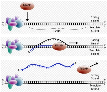
synthesis. Transcription is performed by the enzyme RNA Polymerase, a multi-component protein, found in all living cells. RNA Polymerase binds to promoter region of genes in the presence of specific transcription factors (TFs), and initiate transcription at the start site (Figure 1.6).

TFs are DNA binding proteins that recognize specific binding regions in the promoter or enhancer region of genes. In eucaryotes, TFs can be generic like TATA Binding Factor (TBF), or can be specific, like STATs, targeting a restricted set of genes. Each gene posesses binding sites of a specific set of TFs in their promoter, thus needs presence of a specific set of factors for their expression.

At any given time, depending on the context and cellular stimuli, a tran-scription factor will affect only of a subset of its all possible target genes. This specificity is often provided by modulators, proteins that control transcription fac-tor activity through several different mechanisms, including: post translational modifications, protein degradation, and non-covalent interactions. Modulators help a cell to combine different external signals and make complex downstream decisions. Elucidating their function is necessary for understanding and control-ling cell’s response to external stimuli at gene expression level.

CHAPTER 1. INTRODUCTION 7

Figure 1.6: Sketches showing transcription of a gene. Top: RNA polymerase recognizes the transcription initiation complex, formed by several transcription factors and their binding proteins. Middle: RNA polymerase starts transcrip-tion, reading the coding strand of the DNA and synthesizing mRNA. Bottom: mRNA is synthesized and RNA polymerase dissociated from DNA [80]

1.2.2

Expression Microarrays

The most popular way of detecting gene expression is to measure the mRNA level of the gene. Since mRNAs in a cell are constantly produced and degraded, mRNA concentration cannot last without an active transcription; thus it is an indication of transcription. Translation phase is generally assumed by the pres-ence of mRNA; however, there are studies showing that another kind of RNA, microRNA, can interfere with and inhibit the translation process [54, 67].

Microarray technology is an advancement over the Southern Blotting tech-nique for detecting DNA, and first described by [71]. Southern Blotting is very similar to catching a fish, where the complementary DNA (cDNA) of the queried DNA is bait, and fragmented DNA of the cell separated with gel electrophoresis are the fish [73]. Bait is spread over DNA fragments, and catches (hybridizes with) the DNA whose sequence is complementary. Excess bait is washed out, remaining bait indicates the location of the DNA in query.

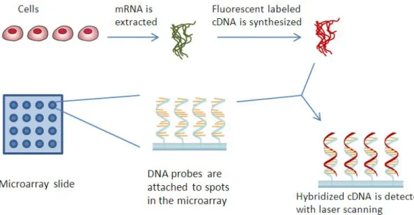
Microarrays detect expression of thousands of genes, sometimes the complete genome of an organism, in a single experiment. The method uses DNA fragments attached to a surface (array). Each spot on the array contains a specific DNA sequence. The mRNA, extracted from the cell, are used for production of labelled with fluorescence cDNAs, which are later hybridized with the DNA attached on the microarray. Attached cDNAs are detected with laser scanning, measuring signals coming from spots, each one indicating the expression level of a gene (Figure 1.7).

There are two main types of microarrays, cDNA arrays and oligonucleotide-arrays. cDNA arrays are historically first emerged type and use the whole ex-pressed sequence as the probe. Each spot cDNA arrays is specific to a gene. Oligonucleotide-arrays, on the other hand, use short oligomers – 25 to 60 bases – in each spot. These oligomers are matched with fragments of genes, one gene represented by several spots on the array. These arrays are mainly produced by corporations Agilent and Affymetrix, they are relatively cheap, and most popular.

CHAPTER 1. INTRODUCTION 9

Figure 1.7: Steps of a microarray experiment

Measured expression values are rarely used as is, since there is no standard for normal expression of a gene. The most common method used for interpreting gene expression is to perform the microarray experiment for two different con-ditions, and compare expressions of the same gene in these conditions. If there is a significant difference in the expressions, then the gene is said to be differen-tially expressed. However, comparing just two arrays for assessing differendifferen-tially expressed genes would not be wise because expression values have high variation due to the expreimental technique. It is said that, differential expressions can be false positive up to 75% [2]. A way to overcome this problem is to perform many microarray expreiments on the same condition and decide the expression by evaluating collectively.

1.3

Contribution

In this thesis, we formulate several analysis methods for process description graphs. Chapter 3 discusses the characteristics of process description graphs and describes some graph traversal algorithms adapted to these graphs. We use

these algorithms for answering several biologically relevant questions like paths between molecules or common targets. We discuss the semantics of integrating microarray data to pathways, and define the concept of causative paths that can be used for elucidating dependencies between gene expressions through paths on the network. In Chapter 4, we describe a probabilistic method, GEM [4], for inferring and characterizing modulators of transcription factors based on ex-pression profiles. We treat interacting molecules of transcription factors as po-tential modulators, and use known targets of factors for measuring the depen-dency of factor-target correlation on the modulator expression. In Chapter 5, we present two tools, PATIKAmad [3] and ChiBE [5], that facilitate pathway visualization and analysis. PATIKAmad is the microarray data integration com-ponent of PATIKAweb [28]. ChiBE is a BioPAX pathway editor that represents BioPAX graphs using the process description notation. It also supports local and distant querying of BioPAX models in process description graphs; and adapts PATIKAmad for expression data integration and analysis.

Chapter 2

Related Work

2.1

Biological Pathway Ontologies

Biological pathways are represented in many different forms, mainly determined by the pathway provider itself. Databases that focus on a specific type of net-work use a model which is simplest to fit their data. For instance Database of Interacting Proteins (DIP) [69] represent their data in PSI-MI [41], which covers molecule and interaction details (like reference or evidence), but cannot model reactions, regulations or abstractions.

There are several efforts for integrating pathway data from different sources. Such an effort have to use a model that can accommodate different types of infor-mation. PATIKA project [24] defines such an ontology, and integrates pathway data from BIND [6], HPRD [50], and Reactome [59] databases. BioPAX [25] is another ontology, being developed with community effort, for modeling many kinds of networks, and offered as a pathway exchange language. SBML [44] is a similar project with a focus on simulation. SBGN [53] is another community effort for determining standards of pathway graphical notation.

An extension of graph-based representation, namely hierarchically structured or compound graphs, in which a member of a biological network may recursively

contain a sub-network of other pathway elements, can be used for representing sub-pathways, molecular complexes and subcellular location. Compound graphs also help managing complexity by interactively decomposing a pathway into dis-tinct components or modules [35, 23]. The recently introduced visualization stan-dard SBGN [53] also uses compound graphs extensively.

2.1.1

PATIKA Ontology

In 2000, PATIKA project was launched to create a pathway visualization and analysis platform with a comprehensive database. Towards this goal, the PATIKA ontology [23], that models pathways in two levels of detail, was defined. Less de-tailed first level (bioentity level) includes bioentities and their binary interactions, while the second level (mechanistic level) models mechanistic details of events.

A molecule node in the mechanistic level is called state, and each state is associated with a bioentity, which keeps references to the sequence databases such as Entrez Gene [56] or UniProt [1], and to small chemical databases such as ChEBI [22] or PubChem [15]. States represent molecular state of an entity in a cellular location with some modification, like phosphorylation.

Events in the mechanistic level are modeled with transitions, which have sub-strate, product, activator, and inhibitor edges that link transitions to states (Fig-ure 2.1). Transitions have several types such as chemical modification, complex formation, and transport.

Homologous states and transitions are modeled with homology abstractions (Figure 2.2), and regular abstraction structure is used for defining any kind of groupings, like pathways.

PATIKA ontology can also handle incomplete information using the model elements incomplete state and incomplete transition (Figure 2.3). When any of the incomplete element is associated with an edge, this means that this edge is actually associated with one of the members of the abstraction, but we do not know which one.

CHAPTER 2. RELATED WORK 13

Figure 2.1: Basics of PATIKA ontology [23].

Figure 2.2: Demonstration of the use of homology abstraction in PATIKA ontol-ogy [23].

Figure 2.3: When the associated state is not certain, but a candidate set exists, incomplete states are used in PATIKA ontology for representing this information.

T1 in the drawing is an incomplete state, indicating either S1 or S10 inhibits the

reaction [23].

2.1.2

BioPAX

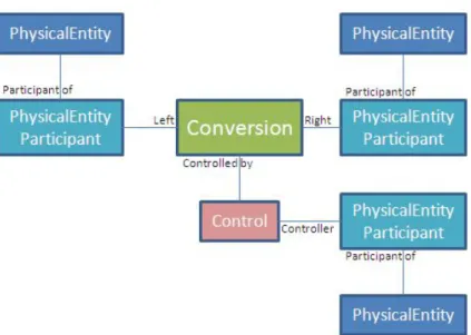
BioPAX (Biological Pathway Exchange Language) project was initiated for cre-ating a common format that will facilitate the data transfer between biological pathway databases. Each version of BioPAX language is called a level. The first BioPAX level (level 1) is released in 2004, modeling biochemical reactions (Fig-ure 2.4). Their model associates PhysicalEntity objects (molecules) to Con-versions through utility objects called PhysicalEntityParticipant, which also keeps stoichiometry, cellular location, and chemical modifications of the associ-ated PhysicalEntity. Level 2 was released with an extension to include physical interactions between molecules.

BioPAX level 3 improves over the previous levels by explicitly putting molecu-lar states in the model. This level completely abandons PhysicalEntityParticipant, and changes semantics of PhysicalEntity to represent molecular states in-stead of entities, and semantics of previous PhysicalEntity class migrates to EntityReference (Figure 2.5). Level 3 also supports gene regulatory interac-tions and genetic interacinterac-tions. Figure 2.6 shows the progress of BioPAX language over time.

CHAPTER 2. RELATED WORK 15

Figure 2.4: Part of the data model of BioPAX Level 1.

Figure 2.6: Progress of BioP AX language as new lev els are released [10].

CHAPTER 2. RELATED WORK 17

Figure 2.7: A manually drawn pathway appeared in [42].

2.1.3

SBML

SBML [44] was developed as a modeling standard for pathways at the level of biochemical reactions. Focus of SBML is simulation of the modeled events; thus, their model is very low level. Each pool of chemically identical molecules in a specific cellular compartment is represented with a Species, which are also inputs and outputs of the Reactions. SBML has structures for reaction rules and parameters, while it completely ignores any generalizations or incomplete information.

2.1.4

SBGN

Biological pathways are generally visualized using graphical models. Most graph-ically pleasing pictures are still manually drawn ones that generally appear in published materials. However, these nice pictures generally lack a consistent no-tation, and it is impossible to understand them without an explanatory text. For instance, the graph in Figure 2.7 describes regulation of Stat signaling by ITAM-dependent pathways [42]. Two arrows that go to Stat1 have completely different meanings. One edge is for the activation of Stat1, while the other is helping this event, which we only understand after reading the related paper.

SBGN [53] is a standardization effort for pathway drawings. It aims the draw-ings to be self-explanatory and to cover most of the biological phenomena. SBGN defines three kinds of drawings: process diagrams, entity relationship graphs, and activity flow graphs. For each graph type, several glyphs are defined as units of the notation. Process diagrams (Figure 2.8) explicitly draw processes with par-ticipant molecular states. This graph type is most similar to the notation used by popular pathway databases like Reactome, KEGG, and PATIKA. Entity re-lationship diagrams (Figure 2.9) draw each entity once, and show processes by edges between entities, their features, and other edges.

2.2

Pathway Editors

A limited number of software tools for biological pathway visualization and anal-ysis was developed such as Cytoscape [51], CellDesigner [36], PATIKAweb [28], Pathway Tools [49], and VisANT [43]. These tools differ in their focus and ca-pabilities. Several of these tools are compared in Table 2.1 with their support to BioPAX and SBGN standards, layout capability, compound graph support, availability and type of software. More details about Cytoscape, CellDesigner, and PATIKAweb are given below.

CHAPTER 2. RELATED WORK 19

Figure 2.8: Stimulation events in the neuro-muscular junction, drawn as a SBGN Process Diagram [70].

Figure 2.9: SBGN entity relationship diagram describing the effect of a depolar-ization (dV) on the intracellular calcium, that binds to calmodulin, that itself binds to the calcium/calmoduline kinase II (CaMKII) [70].

CHAPTER 2. RELATED WORK 21 BioP AX Supp ort La y out Comp ound Supp ort SBGN Av ailab ilit y T o ol T yp e Cytoscap e [51] Y es Automated No No Op en Source Application BiNoM [82] Y es Automated No Y es Op en Source Application 1 Reactome [59] No Automated No Planned Op en Source W eb KEGG T o ols [46] No Man ual/Static Limited 2 No F ree W eb BioCyc [47] Exp ort O nly No No No F ree Application VisANT [43] Y es Y es 3 Y es No Op en Source Application, Applet CellDesigner [36] No Y es Y es Y es F ree Application P athCase [30] Y es 4 Y es No No TSS License 5 Application VISIBIO web Y es Y es Y es Y es Op en Source W eb P A TIKA web [28] Y es Y es Y es No TSS Lisence W eb 1 BiNoM is a plug-in for Cytoscap e 2 Only cellular lo cations are represen ted as comp ounds; complexes are sho wn with simple no des 3 Comp ound supp or t in the la y out seems unreliable 4 BioP AX supp ort seems unrelia ble 5 T om Sa wy er Soft w are License is required T able 2.1: A comparison of sev era l p opular path w a y visualization to ols [26].

2.2.1

Cytoscape

Cytoscape is an open source pathway editor, based on yFiles graph editing frame-work. The project aims the tool to be easily extendable by plugins, so that re-searchers can write their own analyzers for pathways. Today, there are many Cytoscape plugins, written by different groups, implementing a diversity of

path-way analysis algorithms1_.

One pitfall of Cytoscape is that they do not make use of compound graphs, so they have an unusual way of representing complex molecules (Figure 2.10). Cellular locations are shown as text next to the name of the related molecule.

2.2.2

CellDesigner

CellDesigner [36] is a diagram editor for drawing gene-regulatory and biochemical networks. They use SBGN Entity Relationship and Process Diagram representa-tions in drawings (Figure 2.11), and they can save the created models in SBML language. CellDesigner lets user to adjust kinetic parameters of the reactions and concentrations of the molecules, and performs simulations on the model.

2.2.3

PATIKAweb

PATIKAweb [28] is the front-end of the PATIKA database [24]. It is a web based pathway editor, which was built on JSP (JavaServer Pages technology) edition of the Tom Sawyer Visualization technology. Pathway representations are similar to SBGN Process Diagrams. PATIKAweb draws pathways on a cell model; i.e., drawing area is divided into compartments representing cellular locations (Figure 2.12). The tool uses compound nodes for displaying molecular complexes, homologies, and abstractions. Graphs are laid out using the CoSE algorithm [29], specially designed for graphs with compound structures.

CHAPTER 2. RELATED WORK 23

Figure 2.10: Cytoscape pathway showing dissociation of CAV1 from a big com-plex.

Figure 2.11: A screenshot of CellDesigner [14].

CHAPTER 2. RELATED WORK 25

2.3

Reverse Engineering of Gene Regulatory

Networks

Identification of a gene’s regulatory process with controlled experiments is a costly procedure, which requires experiment setups that should involve the gene’s pro-moter with a reporter, and all related transcription factors and their potential

modulators. Since it is not practical to test all potential regulators in

com-binatorially many settings, studies generally focus on few regulators in limited conditions.

Gene expression microarrays can measure expression levels of all genes in a specific condition, thus have potential to provide insights on dependencies of genes to each other for expression. There are many studies that try to re-construct the gene regulatory network using large numbers of expression data. A review by Margolin and Califano [57] classifies reverse engineering methods as linear, probabilistic, and information theoretic, basis of which are summarized below.

All of these methods assume that expression of a gene is a function of other genes, and expression of genes are indicator of their protein activity.

2.3.1

Linear Models

Gene expression at time t+1 can be formulated as the linear combination of other genes’ expressions at time t plus some constant (Eq. 2.1).

xt+1_i =X

j

ajxtj+ ci (2.1)

Xt+1= A × Xt+ C (2.2)

The relation is more formally represented using matrices, like in Eq. 2.2, where, X is the gene expression vector of size n, A is a n × n matrix, and C is

the constants vector of size n. This formulation comes natural when worked on time-series expression data, where samples in the expression dataset belong to equally distributed time intervals, starting after a perturbation is applied to the system.

2.3.2

Probabilistic Models

Probabilistic frameworks try to estimate a probability of expression for the gene under condition of the expression status of other genes. The most popular prob-abilistic framework is the Bayesian network, which is a directed acyclic graph, where nodes represent gene expression statuses and edges represent dependencies

between expressions. A sample formulation is given in Eq. 2.3, where xi is the

expression status of the ith _{gene, π}

i,j represents the jth parent of ith gene, ai,j is

the weight of the effect of jth _{parent on i}th _gene.

P (xi) =

X

j

ai,jπi,j+ ci (2.3)

Probabilistic approaches are generally applicable when gene expressions can be discretized, like high and low. While working on steady-state expression datasets of differing conditions, probabilistic framework is easier to use than a linear sys-tem because of absence of time in the formulation.

2.3.3

Information Theoretic Models

The information theoretic measure, mutual information (MI), can capture the dependency between gene expressions. MI is calculated using independent and joint entropies of gene expressions as in Eq. 2.4, where, S is the information

theoretic entropy, and Xi is the expression vector of the ith gene.

CHAPTER 2. RELATED WORK 27

MI is similar to Pearson correlation in the sense that it measures a kind of dependence between variables; however, Pearson correlation assumes a linear relationship between variables while MI measures any kind of dependence. MI is guaranteed to be non-zero unless variables are statistically independent.

2.4

MINDY - Identifying Transcription factor

modulators

Wang et al. propose an information theoretic approach for inferring modulators of transcription factors (TFs) from microarray data. They measure the mutual information between the TF and the target gene (t ), conditional to the modulator candidate (M ); i.e., CM I(T F, t|M ). The mutual information between TF and the target gene indicates dependency of expression of the target gene on the expression of the TF. In the presence of a modulation, they expect this value to be different in low and high values of the modulator (Eq. 2.5), and infer modulators with a high ∆CM I.

∆CM I = CM I(T F, t|M +) − CM I(T F, t|M −) (2.5)

They test their method on B cells, 254 expression profiles, and identify modu-lators of Myc oncogene. They test all genes as potential targets, and all signaling proteins and other TFs as potential modulators. Low and high values of a mod-ulator are determined by rank-ordering the expression data values, selecting first quartile as low and third quartile as high, and not using the second quartile. Among 542 signaling proteins and 598 transcription factors, MINDY identifies 91 signaling proteins and 99 TFs as modulators of Myc.

Analysis of Process Description

Graphs

This chapter provides the theoretical basis for pathway analysis as implemented in the software tools PATIKAmad and ChiBE.

3.1

Basics

Let G = (V, E) be a graph with a non-empty node set V and an edge set E. An edge, e = x, y or simply xy, joining nodes x and y is said to be incident with both x and y. Node x is called a neighbor of y and vice versa. A pathway graph G = (V, E) is a graph, where some of the edges in E are marked as inhibition edges (e.g., an interaction that disables or impedes the target reaction node via the source state node).

A path between two nodes n0 and nk is a non-empty graph P = (V0, E0) with

V0 = n0, n1, ..., nk and E0 = n0n1, n1n2, ..., nk−1nk, where ni are all distinct. n0

and nk are called the end points of path P = n0n1...nk, whose length, denoted by

|P | is the number of edges on it. A path is said to be directed if all its ordered edges are directed in the same direction. A directed path P is called an incoming

CHAPTER 3. ANALYSIS OF PROCESS DESCRIPTION GRAPHS 29

(outgoing) path of node n if P ends at target (starts at source) node n. A directed path is called positive (negative) if it contains an even (odd ) number of inhibitors (i.e., inhibition edges).

Given node sets A and B, an A − B path is a path with its ends in A and B, respectively, and no node of P other than its ends is from either set A or B. An A − path is a path where one of its end nodes is in A, and no other nodes and interactions are from A.

The graph-theoretic distance dG(x, y), between two nodes x and y in graph

G, is the length of a shortest x − y path in G. If G0 = (V0, E0) is a subgraph of

G = (V, E), and G0 contains all the edges xy ∈ E with x, y ∈ V0, then G0 is an

vertex-induced or simply induced subgraph of G; we say that V0 induces G0 in G

and write G0 = G[V0]. If node x is the starting node of a directed path that ends

up at node y, then node y is said to be in the downstream of node x; similarly, node x is said to be in the upstream of node y. A node y in the downstream of a node x is a potential target of x; similarly, x is a potential regulator of y.

The graph type assumed in the rest of this Chapter (except section 3.5) is bi-ological graphs that are similar to PATIKA mechanistic graphs or SBGN process diagram, which we call process description graph. The characteristic property of such graphs is that they follow the biochemical reaction paradigm, events are represented with a special node type (transitions in PATIKA), molecule nodes, or states, are related to the events through input, output, and effector relations (Figure 3.1).

Edges in a process description graph always have a direction. When two states are connected through a directed path, this implies that the state at the start of the path can have influence on the existence (or concentration) of the state at the end of the path. For instance, in Figure 3.1 the path from S1 to S4 implies that concentration change of S1 can affect the concentration of S4. Because of the presence of such a path, we say that S1 is at the upstream of S4, and S4 is at the downstream of S1.

Figure 3.1: Sample process description graph with three different node types and 5 different edge types. Direction of the edges without an arrow is from the state to the non-state node. Green edge is for activation, while red edge represents inhibition.

Only the effector edges in a process description graph can be negative. In Fig-ure 3.1 S1 is at the positive upstream of S4, and S4 is at the negative downstream of S5.

3.2

Visualization of BioPAX Using Process

De-scription Graph

BioPAX language have some structural differences from process description

graphs, which needs a conversion before visualization and analysis. BioPAX

level 2 uses PhysicalEntityParticipant (PEP) objects as a link from PhysicalEntity (PE) to Interaction (Conversion and Control) objects. PEPs in BioPAX are not reusable objects, they are created per interaction, because PEPs also store the stoichiometry information which is specific to the Interaction. During conversion, each PEP that has the same modification features and the same cellular compartment corresponds to a unique state in process description graph (Figure 3.2).

Conversion in BioPAX can be bidirectional (reversible), however a transition in process description graph is strictly unidirectional. Any reversible Conversion in BioPAX is represented with two transitions in process description graph (Fig-ure 3.3).

CHAPTER 3. ANALYSIS OF PROCESS DESCRIPTION GRAPHS 31

Figure 3.2: PEPs in BioPAX level 2 graph are grouped according to their modifi-cations and cellular lomodifi-cations during conversion. Each group is represented with a unique state in the process description graph.

Figure 3.3: Reversible Conversion in BioPAX is represented with two transitions in process description graph.

Figure 3.4: Desired distance labeling in a process description graph when states are in focus of the traversal. Nodes and edges on the S1-S3 path is labeled according to the distance from S1 (upper labels, forward distance), or distance from S3 (lower labels, backward distance). Distances are defined between states, however, there are advantages of defining distance labels for all nodes and edges. For instance, the sum of forward distance and backward distance of a node or edge on the S1-S3 path is equal to the state-based length of the path, which is 2.

3.3

Paths and Distances

Distances between nodes are often used in graph traversal algorithms. For in-stance the breadth-first search (BFS) guarantees that no node in diin-stance i + 1 will be traversed before all nodes in distance i is traversed. When a graph has a single type of node and a single type of edge, distance between two nodes is simply calculated by the number of the edges on the path that connects them. However, when node and edge types are multiple, distances between a node type of focus can be different from the graph theoretical distance. In that case, we need to modify graph traversal algorithms to run using the specific node-based distance.

In process description graphs, molecular states are connected through other non-state nodes, like transition and control nodes. When the focus of a traversal algorithm is the molecular states on the network, it needs to define the distance as the distance between states. For instance in Figure 3.1, S5 – the upstream inhibitor of S4 – has a graph theoretic distance of 3 from S4. However, S5 is an immediate inhibitor of S4, and the state-based distance is 1.

Figure 3.4 shows an example state-based distance labeling on a path whose graph theoretical distance is 5. The state-based distance from S1 to S3 is 2 because they are connected by 2 events. Here, the non-state nodes and edges

CHAPTER 3. ANALYSIS OF PROCESS DESCRIPTION GRAPHS 33

between states get the label of the state at their upstream. Upper labels in the figure show a forward labeling, i.e, distance from S1; while the lower labels show a backward labeling, i.e., distance from S3. The sum of forward label and backward label of an object on the path is equal to the state-based length of the path, which is 2 in this example.

3.4

Querying Paths on a Network

We previously designed a graph-theoretic querying framework, answering some important biological questions for PATIKA (mechanistic and bioentity) graphs [27], such as neighborhood, shortest path, graph of interest, paths of in-terest, and common stream. Algorithms implemented in this framework did not have to consider the heterogeneity of node types because PATIKA mechanistic graphs are bipartite; thus state-based distance of a path is always half of its graph theoretic distance.

Here we generalize these algorithms to process description graphs, which are not necessarily bipartite; however, node types can be labeled as state and non-state. All these algorithms are based on breadth-first search (BFS), so we first modify the well-known BFS to use the state-based distances in process description graphs, and then build other algorithms on this modified BFS.

3.4.1

BFS for Process Description Graphs

Algorithm 1 is a modified BFS, where search starts from the source set S, ends in target set T, runs in the direction specified by dir parameter, and continues until the limit distance k is reached. If there is no target set, T can be left empty; and if there is no search distance limit, k can be defined as infinite. The complexity of this modified BFS is the same with the ordinary BFS, which is O(|V | + |E|) time complexity, where |V | and |E| are the number of nodes and edges, respectively.

with the closest level of states. This is realized by using a priority queue instead of a regular queue. States are added at the end of the queue to be processed at as the next breadth (line 25), while non-state nodes are added at the head of the queue to be processed immediately (line 27). This BFS also uses a state-based labeling, like the labeling in Figure 3.4. It increments labels only when reaching a state from an edge during forward traversal (line 18), and when reaching an edge from a state during backward traversal (line 12). The algorithm uses color labels for the processing statuses of nodes: white means not processed, gray means in queue, and black means processed. The algorithm assumes initial node colors are white.

3.4.2

Neighborhood

Neighborhood of a set S of source nodes is defined as:

N B(S, k) = S ∪ {x | x is a node on a S-path P, and |P | ≤ k} ∪ {e | e is an edge on a S-path P, and |P | ≤ k}

Upstream or downstream neighborhoods of states in a process description graph can be queried with simple BFS calls (Algorithm 2).

3.4.3

Paths of Interest

Simplest strategy for searching relations between states is to search paths in between. We define the paths-of-interest (PoI) algorithm for searching paths between two given sets of states – source set S, and target set T – within a search distance limit k. This algorithm does not enumerate paths, but returns a merge graph of the related paths. Paths-of-interest is formally defined as:

CHAPTER 3. ANALYSIS OF PROCESS DESCRIPTION GRAPHS 35

Algorithm 1 BFS(S, T , dir, k) Require: dir is fwd or bkwd

Require: S and T contain only state-node

1: for all vertex n ∈ S do

2: _{n.color ← gray} 3: n.label(dir) ← 0 4: Q ← ∅ 5: R ← S 6: Q.enqueue(S) 7: while Q 6= ∅ do 8: u ← Q.dequeue()

9: for all incident edge e of u going in dir do

10: R ← R ∪ {e}

11: _{if dir = bkwd and u is state-node then}

12: e.label(dir) ← u.label(dir) + 1

13: else

14: e.label(dir) ← u.label(dir)

15: n ← e.otherEnd(dir)

16: _{if n.color = white then}

17: _{if dir = fwd and n is state-node then}

18: n.label(dir) ← e.label(dir) + 1

19: else

20: n.label(dir) ← e.label(dir)

21: R ← R ∪ {n}

22: if n /_{∈ T and (n.label(dir) < k or n is not state-node) then}

23: _{n.color ← gray} 24: _{if n is state-node then} 25: Q.enqueue(n) 26: else 27: Q.addF irst(n) 28: else 29: _{n.color ← black} 30: _{u.color ← black} 31: return R

Algorithm 2 Neighborhood(S, dir, k) Require: dir is fwd, bkwd, or both

1: R ← ∅

2: _{if dir = fwd or dir = both then}

3: _{R ← R ∪ BFS(S, ∅, fwd, k)}

4: _{if dir = bkwd or dir = both then}

5: _{R ← R ∪ BFS(S, ∅, bkwd, k)} 6: return R Algorithm 3 PoI(S, T , k) 1: _{C ← BFS(S, ∅, fwd, k)} 2: _{ResetColors(C)} 3: _{C ← C ∪ BFS(T, ∅, bkwd, k)} 4: R ← ∅

5: for all vertex u ∈ C do

6: _{if u.label(fwd) + u.label(bkwd) ≤ k then}

7: R ← R ∪ {u}

8: return R

An alternative version of the PoI algorithm uses the shortest path distance between source and target sets as the search distance limit. This is useful espe-cially when we do not have any idea on the distances from S to T, so we can not provide a realistic k. So, we define the algorithm PoI-Shortest, searching paths from S to T using a length limit shortest + k (Algorithm 4). Both PoI and PoI-Shortest algorithms have O(|V | + |E|) time complexity.

Algorithm 4 PoI-Shortest(S, T , k)

1: _{C ← BFS(S, ∅, fwd, ∞)}

2: _{ResetColors(C)}

3: _{C ← C ∪ BFS(T, ∅, bkwd, ∞)}

4: R ← ∅

5: _{sd ← min(u.label(fwd) + u.label(bkwd)) where u ∈ C}

6: for all vertex u ∈ C do

7: _{if u.label(fwd) + u.label(bkwd) ≤ sd + k then}

8: R ← R ∪ {u}

CHAPTER 3. ANALYSIS OF PROCESS DESCRIPTION GRAPHS 37

3.4.4

Graph of Interest

Often times researchers do not have source and target sets to search a relation in between, but they have just a set of states, and want to learn if they are related. We define the graph-of-interest (GoI) algorithm for searching any path between a given set of states, within a search distance k, which is in fact a PoI call using the state set as both source and target (Algorithm 5). GoI is defined as:

GoI(S, k) = G [B] , where B = {x | x is on a S-S path P, and |P | ≤ k}

GoI can alternatively use PoI-Shortest for searching paths within a distance of shortest + k.

Algorithm 5 GoI(S, k)

1: return PoI(S, S, k)

3.4.5

Common Stream

There are already a number of algorithms for inferring highly connected or co-regulated subnetworks of cellular interactions and processes often called modules or pathways [13, 81, 9]. When analyzing these modules, we often want to know if there is a process or gene that is upstream of the genes in the module, which can provide a causal explanation for the co-regulation, and ultimately a way to control the module. Similarly, two pathways affecting the same mechanism in the cell is interesting since it suggests that a specific phenotype can have more than one molecular cause. For instance, Engelman et al. [31] discuss that drug resistance in lung cancer is related to an alternative pathway that leads to PI3K activation. Searching for common targets of signaling proteins can help to develop alternative treatment strategies.

Common downstream (upstream) of a source entity set S is the set of poten-tial common target (regulator) entities that are in the downstream (upstream) of

all entities in S. We describe the common-stream algorithm for identifying com-mon upstream and downstream (determined by dir parameter) within a search distance limit k (Algorithm 6). Common downstream is defined as:

CD(S, k) = {x | ∀a ∈ S (∃P | P is a path from a to x, and |P | ≤ k)}

Common upstream is defined similarly. The algorithm simply executes a BFS search from each source node and increment reached count of the nodes in the resulting BFS tree. When a node is reached from all of the source nodes, it is collected in the resulting common stream. This algorithm has O((|S|×|V |)+|E|) running time complexity.

Algorithm 6 CommonStream(S, dir, k) Require: dir can be fwd or bkwd

1: C ← R ← ∅

2: for all vertex u ∈ S do

3: _{C ← BFS({u} , ∅, dir, k)}

4: for all vertex n ∈ C do

5: n.reached ← n.reached + 1

6: _{ResetLabel(C, dir)}

7: _{ResetColor(C)}

8: for all vertex v ∈ C do

9: if v.reached = |S| then

10: R ← R ∪ {v}

11: return R

3.4.6

Inter-Compartment Paths

A signal in or outside of the cell is transmitted through cellular locations towards its destination. This is mainly controlled through receptors on the boundary sur-faces of compartments, and carrier molecules that assist other molecules in their transmission. Paths between different cellular locations often capture these sig-naling events. We define Inter-compartment-paths query (Algorithm 7) as a spe-cial application of paths-of-interest query. This query executes a paths-of-interest query from states in a compartment to the states in the other compartment.

CHAPTER 3. ANALYSIS OF PROCESS DESCRIPTION GRAPHS 39

Algorithm 7 InterCompartmentPaths(compartment 1, compartment 2, k)

1: S ← states in compartment 1

2: T ← states in compartment 2

3: _{return PoI(S, T , k)}

3.5

Expression Data on Pathways

Microarray experiments take a snapshot of the cell, showing expression of almost the entire genome. Since gene expressions can be affected from their upstream in a cellular network, and since they can affect expression of their downstream, analyzing expression data on pathways can be informative. One of the simple way of integrating expression data with pathways is visualization of data values on the molecule nodes of the network.

Visualization of expressions on pathways needs a mapping from expression values to molecules in the pathway. This mapping can be obtained by matching external references on the expression data and pathway. However, often times more than one row of expression data match with a molecule on the pathway, and these rows can have dramatically different values. Presence of multiple rows per gene is generally due to presence of several isoforms of that gene, which are measured separately on the expression profile. The most accurate way of visual-ization in that case is to represent all the related values on the molecule nodes; however, this is generally not a practical solution because of space limitation and increasing visual complexity of the pathway drawing. An approximation is to dis-play only the highest value that is matched with the molecule; so that we define expression of a gene as the expression of at least one of its isoforms. This ap-proximation fails when isoforms have different functions, but this time the cause of the failure is not incorrect mapping but absence of sufficient details on the network.

Expression data is a measure for the concentration of RNA molecules in the cell. Thus, the correct way of mapping is to map expressions to RNA states on the network. Unfortunately, RNA states are highly under-represented in popular pathway databases. Representing expressions on the protein states is the next

option, and applied by several pathway editors [51, 5]. When represented on proteins, expression values tend to be interpreted as indicators of protein levels, or activities in the cell. This is a kind of an approximation ignoring translational and post-translational control of proteins, which is probably wrong in many cases, requiring caution when used.

Visualizing a single profile is generally not very informative since expression values do not tell much about activity of gene products. However, comparisons between two profiles tell many things; a change in expression values is often interpreted as a change of activity of gene products in the same direction.

3.6

Causative Paths

Pathway databases contain information about possible interactions and reactions between molecules in a cell. Usually, this data is created by manually curating biological literature and can span multiple experiments from different tissues, organisms and contexts. When taken as an interconnected network, these inter-actions and reinter-actions offer a causal model of a cell’s response to stimuli. For instance, in a typical microarray experiment, relatively small portions of this network are differentially active between the control and the sample, and deter-mining these parts can be extremely useful for finding causal explanations for the correlations observed in the data.

Change of an expression value can be related to change of other gene expres-sions through a path in the cellular network. If a path in the network potentially explains expression change of the end-state with the expression change of the start-state, then we call it a causative path.

The last transition in a causative path should be a transcription, or should at least be related to gene expression. A positive causative path will have similar expression changes at its start-state and end-state. Similarly, a negative path can be causative only when it has different expression changes at its start-state and end-state (Figure 3.5).

CHAPTER 3. ANALYSIS OF PROCESS DESCRIPTION GRAPHS 41

Figure 3.5: Examples of two causative paths. Red state: upregulated, blue state:

downregulated. Transitions with label t are transcription events. Red edge:

Discovering Modulators of Gene

Expression

Our current knowledge of the modulation of transcription factors comes mainly from experimental studies that measure the expression levels of a few target genes (such as [62] and [66]) or the expression level of an artificial reporter gene with a “canonical promoter” (such as [77]). While these experiments provide invaluable insight, they do not tell the whole story. In order to detect context-dependent, target-specific effects of modulators, system-scale methods are required. Gene expression profiles are now extensively used for inferring causal relationships be-tween transcription factors and target genes. The models produced from gene expression profiles, often referred as “gene regulatory networks”, or simply “gene networks”, differ significantly in their semantics and level of detail. Margolin and Califano [57] provide a comprehensive review of these methods and classify them under three groups: linear, graph-theoretic, and information-theoretic models (Section 2.3). The majority of these methods focus on modeling either causal relationships between gene expression levels as binary interactions, or linear in-tegration of expression values.

Expression level of genes can also be affected by non-modulator proteins such as alternative transcription factors, generic inhibitors of transcriptional machinery

CHAPTER 4. DISCOVERING MODULATORS OF GENE EXPRESSION 43

or regulators of mRNA degradation. A modulator is defined by its dependency on the transcription factor in order to exert its effect on the target. When the transcription factor is not present, at least a part of the modulator activity should be rendered ineffective. This implies a ternary, non-linear relationship, analogous to the electrical transistor, between the activity levels of the two “inputs”, the transcription factor and the modulator, and the “output”, the target gene expres-sion. Using a sufficiently large set of expression profiles, these relationships can be detected by looking at the correlations between expression levels of candidate modulators with the expression level of a transcription factor and its target genes. Assuming that the expression level is an indicator of modulator and transcription factor activity, the dependency between modulator and target expression must increase as the concentration of the transcription factor increases. Therefore, we expect to observe a transcription factor-dependent correlation between modulator and target.

Wang et al. [76] propose MINDy, an information theoretic algorithm for de-tecting modulators. They test the conditional mutual information (CMI) between the transcription factor and the target gene, and its dependency on the modula-tor candidate (Section 2.4). This is, in essence, the aforementioned non-linearity principle. Building upon the same principle, we present GEM (Gene Expression Modulation) [4], a probabilistic method for detecting modulators of transcription factors using a priori knowledge and gene expression profiles. For a modulator / transcription factor / target triplet, GEM predicts how a modulator-factor inter-action will affect the expression of the target gene. GEM improves over MINDy by detecting two new classes of interaction that would result in strong corre-lation but low ∆CMI, can filter out logical-or cases and offers a more precise classification scheme. A detailed comparison of GEM and MINDy is provided in Section 4.2.2.

In the following sections, we explain our method and assumptions and apply GEM to predict modulators of Androgen Receptor (AR). We compare our results with a recent literature review on modulators of AR and show that GEM correctly predicts a significant number of its modulators and can provide additional insight into the mechanism of modulation and affected targets. We observe that these