Journal of Physics: Condensed Matter
TOPICAL REVIEW
Beyond Poisson–Boltzmann: fluctuations and fluid
structure in a self-consistent theory
To cite this article: S Buyukdagli and R Blossey 2016 J. Phys.: Condens. Matter 28 343001
View the article online for updates and enhancements.
Related content
Electrostatic interactions in charged nanoslits within an explicit solvent theory
Sahin Buyukdagli
-Ion size effects upon ionic exclusion from dielectric interfaces and slit nanopores
Sahin Buyukdagli, C V Achim and T Ala-Nissila
-Dipolar depletion effect on the differential capacitance of carbon-based materials
Sahin Buyukdagli and T. Ala-Nissila
-Recent citations
Modeling electrokinetics in ionic liquids
Chao Wang et al
-Journal of Physics: Condensed Matter
S Buyukdagli and R Blossey
Beyond Poisson–Boltzmann
Printed in the UK 343001 JCOMEL © 2016 IOP Publishing Ltd 2016 28
J. Phys.: Condens. Matter
CM
0953-8984
10.1088/0953-8984/28/34/343001
34
Journal of Physics: Condensed Matter
1. Introduction
Poisson–Boltzmann (PB) theory is the cornerstone of soft mat-ter electrostatics, but in recent years several shortcomings of this theory have also been clearly revealed. PB theory is a mean-field theory, hence it neglects all fluctuation or correlation effects, and as a simple continuum theory it also ignores the structure of solvents and ions. In the presence of ions of high valency, prominent in biological systems in particular, the theory even fails qualitatively. A systematic field-theoretic approach to soft matter electrostatics developed with the counter-ion case has allowed the identification of a coupling parameter [1],
σ β πε Ξ ≡ | | = q e q 8 3 4 2 2 2 B CG (1)
where q is the valency of the counter-ions, σe is the surface charge density with the electronic charge e, ε is the dielectric constant, and β = k T1/ B . Ξ is thus essentially the ratio of the
Bjerrum length B=e2/(4πε ε0 wk TB ) and the Gouy–Chapman
length GC=1 2/( π qB | |σs). Poisson–Boltzmann theory is the weak coupling limit Ξ→0 of the more general theory, while for Ξ→∞, the strong coupling case, a single-particle picture emerges [2].
Even within the weak coupling limit, or for intermediate values of the coupling parameter, Poisson–Boltzmann theory does not fully describe the electrostatic phenomena in soft matter systems. Being a mean-field theory, it entirely lacks the correlation effects between the charges. These are, however, crucial in many physical settings. For the case of electrostatics near macromolecular surfaces or membrane interfaces—one
Beyond Poisson
–Boltzmann: fluctuations
and fluid structure in a self-consistent
theory
S Buyukdagli1 and R Blossey2
1 Department of Physics, Bilkent University, Ankara 06800, Turkey
2 University of Lille 1, CNRS, UMR 8576 UGSF—Unité de Glycobiologie Structurale et Fonctionnelle,
59000 Lille, France
E-mail: [email protected]
Received 28 December 2015, revised 11 April 2016 Accepted for publication 25 May 2016
Published 30 June 2016
Abstract
Poisson–Boltzmann (PB) theory is the classic approach to soft matter electrostatics and has been applied to numerous physical chemistry and biophysics problems. Its essential limitations are in its neglect of correlation effects and fluid structure. Recently, several theoretical insights have allowed the formulation of approaches that go beyond PB theory in a systematic way. In this topical review, we provide an update on the developments achieved in the self-consistent formulations of correlation-corrected Poisson–Boltzmann theory. We introduce a corresponding system of coupled non-linear equations for both continuum electrostatics with a uniform dielectric constant, and a structured solvent—a dipolar Coulomb fluid—including non-local effects. While the approach is only approximate and also limited to corrections in the so-called weak fluctuation regime, it allows us to include physically relevant effects, as we show for a range of applications of these equations.
Keywords: electrostatics, self-consistent theory, correlation effects (Some figures may appear in colour only in the online journal)
Topical Review
IOP
doi:10.1088/0953-8984/28/34/343001
of the most basic situations encountered in soft matter—this omission does not allow the image charge effects of solvated ions to be treated. Another crucial effect is the charge reversal of macromolecules induced by the overscreening of their bare charge by multivalent counter-ions. This effect can indeed modify the interactions between charged objects, even in a qualitative way.
Therefore, in order to remedy this deficit, methods to include fluctuation effects have been devised. In this topical review, we deal exclusively with one such approach, which relies on a variational formalism, leading to self-consistently coupled equations of the electrostatic potential and its cor-relation function. The formulation that we base this on was originally introduced by Netz and Orland [3], following ear-lier work by Avdeev et al [4]. More precisely, Netz and Orland used the variational approach to calculate the mean-field level charge renormalization associated with the non-linearity of the Poisson–Boltzmann approach, without considering the correlation effects embodied in the self-consistent equations.
In recent years, the variational approach has, however, seen a number of physically relevant applications, covering differ-ent charge geometries, and even dynamical situations such as flow-related effects in nanopores. Hatlo et al considered the variational formulation of inhomogeneous electrolytes by introducing a restricted self-consistent scheme [5]. In [6, 7], one of us (SB) introduced a numerical scheme for the exact solution of the variational equations in slit and cylindrical nanopores. At this point, we should also mention the one-loop treatment of charge correlations that allows the analyti-cal treatment of inhomogeneous electrolytes. Netz introduced the one-loop calculation of the ion partition at membrane sur-faces in counter-ion-only liquids [8]. This was subsequently extended by Lau [9] to electrolytes symmetrically partitioned around a thin charged plane. In [6], we integrated the one-loop equations of a charged liquid in contact with a thick dielectric membrane. Finally, in [10, 11], we considered the role played by charge correlations on the electrophoretic and pressure-driven DNA translocation through nanopores.
In addition, while the original self-consistent equations only covered the case of systems that can be described by mac-roscopic dielectric constants, modified equations have been derived that can also include the effects from fluid structure. The first dipolar Poisson–Boltzmann theory including solvent molecules as point-dipoles was introduced in [12]. Abrashkin
et al incorporated excluded volume effects into this model [13]. One of us (SB) derived a Poisson–Boltzmann equa-tion that relaxes the point-dipole approximation and includes solvent molecules as finitely sized dipoles [14]. This model, which also accounts for ionic polarizability, was shown to contain the non-locality of electrostatic interactions observed in molecular dynamics simulations. Finally, we derived the dipolar self-consistent equations of this model, and in this way generalized Netz–Orland’s variational equations for explicit solvent liquids [15].
Our ambition in this topical review is to provide a quick technical introduction to the method and the results that have been achieved with this approach. We have attempted to make this approach accessible to newcomers by giving a sufficient
amount of technical detail for the simpler cases. This level of detail then, by necessity, diminishes for the more complex ones that follow; however, we hope that by that time, a reader willing to go through about the first third of the equations in a stepwise manner will have no difficulty in following the rest of the paper. For the latter part, as in all reviews, we refer our readers to the original articles for further details.
The material presented in the review is organized as fol-lows. In section 2 we derive the model equations which have been called either variational PB equations, self-consistent field equations, or fluctuation-enhanced Poisson–Boltzmann equations (FE-PB), for the case of a system with 1–1 salt. We also discuss the limits of validity that can be expected from the equations. In section 3 we review the results for systems whose dielectric properties can be properly covered by di electric constants. In particular, we discuss situations of high current interest involving the application of the approach to nanopore geometries. Section 4 contains very recent exten-sions of the approach, including the fluctuation-enhanced Poisson–Boltzmann equations for a dipolar solvent, the DPBL-equation, as well as a non-local version of the latter. Section 5 presents a brief summary and outlook. We finally note that we explain, wherever possible at present, the theor-etical results closely in relation to the experimental findings. This is obviously the ultimate way to validate a theory, and the reader is invited to see how far the self-consistent approach to soft matter electrostatics has been carried so far.
2. Fluctuation-enhanced Poisson–Boltzmann equations
2.1. Derivation
The fluctuation-enhanced Poisson–Boltzmann equa-tions result from the observation that a simple perturbative treatment of the non-linear Poisson–Boltzmann equation only has poor convergence properties. This is particularly the case for electrolytes in contact with low permittivity macromol-ecules or membranes where the singularity of the resulting image-charge potential does not allow the one-loop expansion of the grand potential. As in many other branches of physics, variational approaches thus come as an often fruitful alterna-tive. In this vein, the starting point is the Gibbs variational procedure that consists of extremizing the variational grand potential in the form [3] Ω = Ω +v 0 H−H0 0/Ξ, where H0[ ]φ
is a trial Hamiltonian functional and the bracket ⋅ 0 denotes the field-theoretic average with respect to this Hamiltonian. For this Hamiltonian, the most general functional ansatz is a Gaussian one including the mean electrostatic potential Φ and the covariance of the field expressed via its Green’s function
G as variational parameters
∫ ∫
φ = φ + Φ Ξ ′ − φ ′ + Φ ′ ′ H 1 r r Gr r r r 2 r r i , i . 0[ ] [ ( ) ( )]( ( )) [ ( )1 ( )] (2) For definiteness, we now consider the case of monovalent ions with charges ±q confined to a region Ω in the presence of a fixed charge density f. The Hamiltonian is then, following [16][ ] ⎡( ) ( )/ ⎣⎢ ⎤ ⎦⎥
∫
φ π φ φ φ = ∇ + −Λ Ξ H 1 2 r 2 i f 2e cos , G r r 2 , 2 0 (3)where Λ is the fugacity of the ions, and G0(r r, ′)= | − |1/r r′
is the bare Coulomb potential. The introduction of G0 at this level takes care of the regularization of the Green’s function
( )′
G r r, in the final equations as the ionic self-energy corresp-onding to the equal-point correlation function G( )r r, diverges in the present dielectric continuum formalism. In equation (3), this factor shifts the chemical potential of the ions. With this ansatz, we can compute the grand potential Ωv from which the sought equations follow after extremization with respect to the functions Φ and G. These self-consistent equations read as
( ) ( )/ ( ) ( ) ∇ Φ r − Λe−Ξc sinhΦr = −2 r, f r 2 2 (4) πδ ∇ − Λ2 e−Ξcr 2coshΦ r G r r, ′ = −4 r−r′ , [ ( )/ ( )] ( ) ( ) (5) = ′ − ′ ′ cr lim Gr r, G r r, . r r 0 ( ) [ ( ) ( )] → (6) Equation (4) is a modified Poisson–Boltzmann equation, aug-mented by the correlation function (6) in the exponential. The correlation function fulfills a modified Debye–Hückel (DH) equation, equation (5), in which the usual inverse Debye-length κ2 is replaced by a non-linear function of both c( )r and φ r( ).
These equations are one realization (for the case of 1–1 salt, and without further specification of the fixed charge geometries) of the self-consistent or fluctuation-enhanced Poisson–Boltzmann equations. One should also note that equations (4) and (5) can be easily generalized to an asymmetrical electrolyte (see e.g. [7]).
2.2. Validity
The self-consistent equations (4)–(6) are, by their very construc-tion, only approximate. Their validity ultimately rests on the validity of the Gaussian assumption to begin with, and this is, as usual in variational approaches, not always easy to quantify. One can, however, identify the validity regime qualitatively by considering the charge correlations in a bulk electrolyte. In this case, the electrostatic potential φ vanishes and we are left with a
Debye–Hückel type equation for the Green’s function [17]
( ) ( )/ ( ) πδ( )
−∇2G r r, ′ + Λe−Ξcr 2Gr r, ′ =4 r−r′ .
(7) If we define the screening parameter as κ ≡ Λ2 e−Ξc( )/r 2, the
Green’s function becomes
( ) = | − | ′ ′ κ − | − |′ Gr r r r , e r r . (8)
Inserting equation (8) into equation (6), one finds c= −κ. We are thus led to a first self-consistency condition given by
/
κ = Λ2 eΞκ2.
(9) This equation ceases to have a solution for large values of the coupling parameter Ξ, clearly indicating that the self-consis-tent equations (5) and (6) are only valid for weak to moderate charge correlations. This condition can be, in turn, quantified through equation (1) in terms of the model parameters.
In inhomogeneous liquids, the validity limit of the self-con-sistent equations (5) and (6) is not so easy to assess, as they are, due to their highly non-linear character, not amenable to ana-lytic solutions, even for simple geometries. Numerical meth-ods have recently been developed to solve them [6, 7, 16, 18]. In particular, in comparison with the MC simulations, [6] and [7] identified the validity regime of the equations for liquids confined to slit and cylindrical nanopores, respectively. In the following we will discuss the approximate solutions of equa-tions (4)–(6) and their modifications to physically relevant situations, which to some extent also permit analytical calcul-ations. In particular, we confront these solutions with data from experiments and simulations.
3. The variational equations for a dielectric continuum
In this section, we turn to the application of the SC equa-tions to some specific physical situations. First, we discuss ion correlations and charge reversal at a planar interface, and then move on to the dynamic effects associated with DNA translocation through membrane pores. These examples were selected as they allow us to convey the main insights about correlation effects that can be gained from the variational approach, and in conjunction with ions of higher valency, where PB-theory is known to fail. Further applications of the equations in the case of a dielectric continuum concern the effect of image charges on macro-ions [19] and on the elec-trical double layer [20, 21]. The ion size effects upon ionic exclusion from dielectric interfaces and slit nanopores were treated in [22–24]. The modification of ion polarizabilities from the gas phase to solvation in polar liquids was discussed in [25].
3.1. One-loop expansion of the SC equations and charge reversal
We begin the discussion with the one-loop (1- ) expan-sion of the electrostatic SC equations, valid exclusively for di electrically continuous systems ε( )r =εw. We consider a symmetric electrolyte composed of two ionic species with valencies ±q and a bulk density ρb. In order to facilitate the link to the research literature, in passing from equation (4) to the subsequent equation (10) we will introduce the definition of the new average potential ψ( )r = − Φq ( )r and the Green’s function v(r r, ′)= ΞG(r r, ′). For this case, the SC equa-tions read as ( ) ( ) ( ) [ ( )] ( ) ψ κ ψ π σ ∇ r − e− − δ sinh r = −4 q r b V q v r r r 2 2 2 , B w 2 (10) ( ) [ ( )] ( ) ( ) ( ) ( ) κ ψ π δ ∇ − = − − ′ ′ ′ δ − − vr r r vr r r r , e cosh , 4 , b V q v r r r 2 2 2 , B w 2 (11) where the ionic self-energy (or renormalized equal-point cor-relation function) is defined by
( ) ( ) ( ) ( ) δvr ≡δvr r, = Bκb+vr r, −vcb0 ,
(12) where the DH screening parameter κb2=8π qB 2, and the
func-tion Vw( )r is the ionic steric potential accounting for the rigid boundaries in the system.
The 1- expansion of these equations consists of Taylor-expanding equations (10) and (11) in terms of the electrostatic Green’s function v(r r, )′. Splitting the average potential into its MF and 1- components as ψ( )r =ψ0( )r +ψ1( )r, for the MF potential and the 1- electrostatic Green’s function equa-tions one obtains ( ) ( ) [ ( )] ( ) ψ κ ψ π σ ∇ r − e− sinh r = −4 r b V r 2 0 2 w 0 B (13) {∇ −κe− ( )cosh[ ( )]} (ψ r vr r, ′)= −4π δ(r−r′), b V r 2 2 0 B w (14) and for the 1- correction to the average potential
κ ψ ψ κ δ ψ ∇ − e− cosh r r = −q − vr r 2 e sinh . b V r b V r 2 2 0 1 2 2 0 w w { ( ) [ ( )]} ( ) ( ) ( ) [ ( )] (15) In order to solve the system of differential equations (13)–(15), we first invert equation (14) and recast it in a more practical form for analytical evaluation. By using the defini-tion of the Green’s function
( ) ( ) ( )
∫
drv− r r, vr r, ′ =δr−r′ ,1 1 1 1
(16) one can invert equation (14) and express the electrostatic ker-nel as π κ ψ δ = − ∇ − − ′ ′ − − v r r, 1 r r r 4 r be V cosh , r 1 B 2 2 0 w ( ) { ( ) [ ( )]} ( ) (17) in terms of which equation (15) can be written as
( ) ( ) ( ) ( ) [ ( )]
∫
drv− r r, ψ r =q ρe− δvr sinh ψ r .b V r
1 1 2 1 1 1 4 w 2 2 0 2
(18) Multiplying equation (18) with the potential v(r r, 2) and
integrating over the variable r2, one finally gets the integral
relation for the 1- potential correction completing the equa-tions (13) and (14) ( )
∫
( ) ( ) ( ) [ ( )] ψ r =ρq d er − vr r, δvr sinh ψ r . b V r 1 4 1 w 1 1 1 0 1 (19) We also note that within 1- -theory, the ion number densities are given by ∓ ∓ ρ =ρ ψ − δ ψ ± − ⎧ ⎨ ⎩ ⎫ ⎬ ⎭ q v r e 1 r r 2 . b V r r 2 1 w 0 ( ) ( ) ( ) ( ) ( ) (20)We now have the main set of equations ready and turn to the analytical solutions of equations (13)–(15) for a simple planar geometry in order to investigate the charge inversion phenom-enon [7]. Then we will couple these equations with the Stokes equation and show that charge inversion gives rise to a rever-sal of electrophoretic DNA mobility [10] and hydrodynami-cally induced ion currents through cylindrical pores [11].
3.1.1. Ionic correlations and charge reversal at planar inter-faces. In this part, we consider the charge reversal effect
in the case of a negatively charged planar interface located at z = 0. The electrolyte occupies the half-space z > 0 while the left half-space at z < 0 is ion-free. In the SC-equations this corresponds to a steric potential Vw( ) = ∞r if z < 0 and
( ) =
Vw r 0 for z > 0. The wall charge distribution function is
( ) ( )
σr = −σδs z. By introducing the Gouy–Chapman length
/( )
µ π σ
≡ =
GC 1 2 q Bs that corresponds to the thickness of the interfacial counter-ion layer, the solution of equation (13) satisfying Gauss’s law ψ′ z 00( = )=2/µ reads as
( ) (( )) ψ = − + − κ κ − + − + ⎡ ⎣⎢ ⎤ ⎦⎥ z 2 ln 1 e 1 e , z z z z 0 b b 0 0 (21)
where we introduced the parameter s=κ µb and the auxiliary functions z0= −ln[ ( )]/γs κb and γ( )s = s2+ −1 1. In the DH-limit of a weak surface charge or strong salt, the potential (21) becomes ψ ( ) ( / )z 2 es −κz
0 b. The parameter s thus
corre-sponds to the inverse magnitude of the surface potential. Taking advantage of the planar symmetry in the (x, y)-plane one can expand the Green’s function in the Fourier basis as
( ′)=
∫
π ( ∥− |∥′)˜ ( ′) ∞ vr r, dkkJ kr r v z z 2 , , 0 0 0 (22) where r∥ is the position vector in the (x, y)-plane and J0 is a Bessel function of the order zero. Substituting the expansion (22) together with the MF-potential (21) into the kernel equa-tion (11), the latter takes the form[ ( ){ [ ( )]}]˜( ) ( ) θ κ κ π δ ∂ − + + = − − ′ ′ z p z z v z z k z z 1 2 csch , , 4 z b b b 2 2 2 2 0 B (23)
where we defined the function pb = k2+κb2. The solution of
equation (23), satisfying the continuity of the potential v z z˜( , ′)
and the displacement field ∂zv z z˜( , ′) at z = 0 and z= ′z reads ˜ ( ′)= π [ ( ) ( )+ − ′ + ∆ −( ) ( )]− ′ v z z p k h z h z h z h z , 2 b 0 B2 (24) for 0⩽ ⩽ ′z z, where the homogeneous solutions of equa-tion (23) are given by
∓κ κ = + ± ± ⎧ ⎨ ⎩ ⎫ ⎬ ⎭ h z p z z e p z 1 b coth , b b 0 b ( ) [ ( )] (25)
and the ∆-function reads
( ) ( )[ ( )] ( ) ( )[ ( )] κ κ κ κ κ κ κ κ ∆ = + − − + + + z p k p z z p k p z csch coth csch coth . b b b b b b b b b b b b 2 2 0 0 2 2 0 0 (26)
For z z⩾ ′, the solution of equation (23) can be obtained by interchanging the variables z and z′ in equation (24). From now on we switch to the non-dimensionalized coordinate
¯ κ=
z bz. Rescaling the wave-vector of the Fourier expansion (22) as k→u=pb/κb as well, and inserting the function (24) into equation (12), the ionic self-energy accounting for the charge correlations takes the form
(¯) { [¯ ( )] ¯ ( [¯ ( )]) ¯ }
∫
δ γ γ = Γ − − − + ∆ + − ∞ − v z u u z s u z s d 1 csch ln coth ln e , c c zu 0 1 2 2 2 2 (27)where we defined the electrostatic coupling parameter κ Γ = B b and ∆ = + − + − − + + + + − s su s u u s su s u u 1 1 1 1 1 1 . 2 2 2 2 ¯ ( )( ) ( )( ) (28)
Inserting the MF-potential (21), the Green’s function (24) and the self-energy (27) into equation (19), and carrying out the spatial integral, the 1- -correction to the average potential takes the form
(¯) [¯ ( )]
∫
(¯ ) ψ = Γ − γ − ∞ z q z s u u F z u 4 csch ln d 1 , , c 1 2 1 2 (29) where we introduced the auxiliary functionγ = + + − ∆ + + + + +∆ − + ∆ − − − ⎛ ⎝ ⎜⎜ ⎞⎠⎟⎟ F z u s s s u u s s s u z s , 2 1 1 2 2 3 1 e uz e uz 1 coth ln . c 2 2 2 2 2 2 (¯ ) ¯ ¯ ( ¯ ) [¯ ( )] ¯ ¯ (30)
We note that the correlation-corrected ion densities (20) are fully characterized by the potentials (21), (27) and (29). One also sees that these functions depend solely on the parameters
s and Γ.
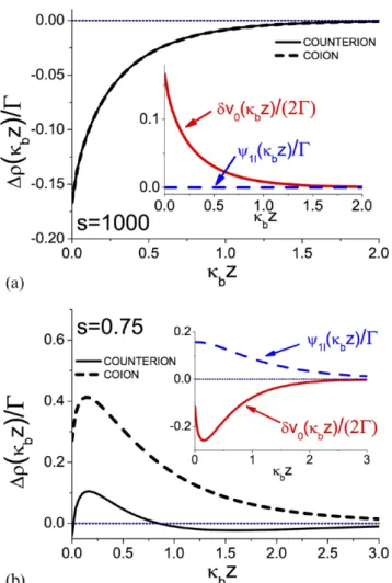
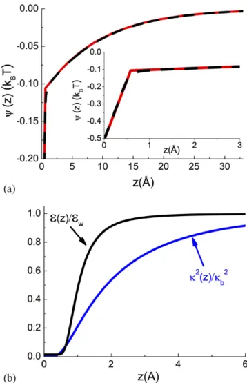
In figure 1, we show the 1- -correction to the ion densities
(¯) (¯) (¯) (¯) (¯)∓ (¯) ρ ρ ρ ρ δ ψ ∆ ± ≡ ± − ± = − ± z z z z q v z z 2 , MF MF 2 0 1 (31)
where the MF-ion densities are given by ρ (¯)=ρ ψ(¯)
± z be∓ z
MF 0 .
The top plot (a) illustrates the density correction at a weakly charged membrane (s = 1000). In this case, the absence of ions in the left half-space results in an ionic screening defi-ciency close to the membrane surface. As a result, ions pre-fer to move away from the interface towards the bulk where they are more efficiently screened and possess a lower free energy. This translates in turn into a positive ionic self-energy
(¯)
δv z0 >0 (see inset) and a decrease in the MF-level co-ion and
counter-ion densities (main plot) by the charge correlations. In the plot of figure 1(b), we consider a strongly charged membrane (s = 0.75). In this parameter regime, the strong counter-ion attraction results in an interfacial charge excess. The ions being more efficiently screened in the vicinity of the membrane surface, they tend to approach the interface. This effect is reflected in the attractive ionic self-energy δv z0(¯)<0
(inset) and the amplification of the MF-density of both co-ions and counter-co-ions (main plot). In [6], it was shown that the transition between these two regimes with the surface self-energy δv 00( ) switching from positive to negative occurs when
the size of the interfacial counter-ion layer becomes compa-rable to the ionic screening radius in the bulk region, i.e. at µ κ −
b1. This equality yields the characteristic membrane charge σ∗= 2ρ π/( )
s b B above which the interfacial
screen-ing dominates the bulk screenscreen-ing.
For a negatively charged membrane, the MF-potential is negative (see equation (18)). Furthermore, in the inset of
figure 1(b) where we plotted the 1- -correction equation (29) to the average potential, one sees that the former is positive. This stems from the interfacial screening excess. Thus, at strongly charged membranes, correlations attenuate the mag-nitude of the negative MF-potential.
We will now show that this peculiarity is the precursor of the charge reversal effect. In order to illustrate this point, we note that at large distances from the charged plane z¯ 1, the MF-potential (21) behaves as ψ(¯)z −4γ( )s e−z¯
0 . Expanding
the 1- -correction to the average electrostatic potential (30) in the same limit, one finds that the correlation-corrected average potential ψ1 (¯)z =ψ0(¯)z +ψ1(¯)z takes the form
ψ z − η − s s 2 e , l z 1(¯) ( ) ¯ (32) where we introduced the charge renormalization factor accounting for electrostatic many-body effects
( ) ( ) ( ) η = γ ⎡ − Γ ⎣⎢ ⎤ ⎦⎥ s 2s s 1 q s 8 I , 2 (33)
Figure 1. One-loop corrections to the counter-ion (solid lines) and
co-ion densities (dashed lines) from equation (31), for two different values of the parameter s=κ µb , the ratio of the Gouy–Chapman and the screening length. Case (a): s = 1000 (a weakly charged membrane) and case (b): s = 0.75 (a strongly charged membrane). The inset shows the ionic self-energy and the one-loop correction to the external potential for these parameters.
with the auxiliary function
∫
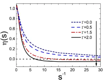
= − + + − − ∆ + + + + ∞ ⎪ ⎪ ⎪ ⎪ ⎧ ⎨ ⎩ ⎛ ⎝ ⎜⎜ ⎞ ⎠ ⎟⎟⎫⎬ ⎭ s u s s s u u s s s I du 1 2 1 1 1 2 2 3 1 . 1 2 2 2 2 2 ( ) ¯ (34) In figure 2, we plot equation (33) versus s−1 for various cou-pling parameters Γ. In the MF-limit Γ = 0, and the charge renormalization factor η s( ) accounts for the non-linearities neglected by the linearized PB-theory. As the latter overesti-mates the actual value of the electrostatic potential at strong charges, with an increasing surface charge from left to right, the correction factor η s( ) drops from unity to zero. Moreover, one sees that at the coupling parameter Γ = 2, the charge renormalization factor passes from positive to negative. In other words, at large distances from the interface, the total average potential (32) switches from negative to positive. This is the signature of the charge inversion effect. As the adsorbed counter-ions overcompensate for the negative fixed surface charge, the interface acquires an effective positive charge. For small s (or large surface charge density), equation (33) takes the asymptotic form( ) ⎡⎣⎢ ( )⎤⎦⎥ ( )
η s =2 1s − Γπ−4 ln 2s +O s
16 .
2
(35)
Setting the equality (35) to zero, one finds that the charge reversal takes place at the particular value
π Γ = − Γ ⎜ ⎟ ⎛ ⎝ ⎞⎠ s 1 2 exp 4 4 . c( ) (36)
Having established the charge reversal effect in the planar geometry, we will now turn to its influence on ion currents and polymer mobilities through cylindrical nanopores, which is a problem of current interest in the field of soft matter physics.
3.1.2. Electrophoretic DNA mobility reversal by multivalent counter-ions. In this part we discuss the effect of charge inversion induced by multivalent ions on the electrophoretic mobility of a DNA molecule [10]. The molecule is modelled
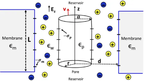
as a charged cylinder with a radius of a = 1 nm, translocating through a nanopore of cylindrical geometry with a radius of
d = 3 nm. The configuration is depicted in figure 3. The solu-tion of the 1- equations (13)–(15) in a cylindrical geometry is similar to their solution in planar geometry. Thus, we will skip the technical details here and refer to [7] and [10] for details. The DNA molecule has a negative surface charge distribu-tion σ( )r = −σ δp (r−a), with σ = 0.4p e/nm2 and r being the radial distance of ions from the symmetry axis of the cylindri-cal polymer. In the general case, the permittivity of the nano-pore εm and DNA may differ from the water permittivity εw. However, in order to simplify the technical task, we assume that there is no dielectric discontinuity in the system and set εm=εp=εw= 80.
As the electrophoretic translocation of DNA under an external potential gradient ∆V corresponds to the collective motion of the electrolyte and the DNA molecule, first we need to derive the convective fluid velocity uc (r) given by the
Stokes equation η∇u r +eρ r ∆V = L 0, c c 2 ( ) ( ) (37)
with the viscosity coefficient of water η =8.91×10⁻⁴ Pa s⋅ ,
the nanopore length L, and the liquid charge density
( )
∑
( )ρcr = qρ r ,
i i i
(38) where ρ ri( ) is the number density of the ionic species i with valency qi, ( ) ( )⎡ ( ) ( ) ⎣ ⎢ ⎢ ⎤ ⎦ ⎥ ⎥ ρ r =ρ e− ψ 1−qψ r −q δv r 2 . i ib q r i 1 i 2 i 0 (39)
By making use of the Poisson equation ∇2ψ1 ( )r +4π ρ Bc( )r =0 in equation (37), the latter can be written explicitly in the cylindrical geometry as η ε ψ ∂ ∂ ∂ ∂ − ∆ ∂ ∂ ∂ ∂ = r rr ru r k T er V L rr r r r 0. c( ) B ( ) 1 ( ) (40) In order to solve equation (40), we first note that the 1- - potential ψ1 ( )r satisfies Gauss’s law φ′ a( )=4π σ B p at the DNA surface. In the steady-state regime, where DNA translocates at a constant velocity v, the longitudinal electric force per poly-mer length Fe= −2π σae p∆V L/ will compensate for the
vis-cous friction force Fv=2π ηa u a′c( ), that is Fe+Fv=0. Finally, we impose the boundary conditions uc(d) = 0 (no-slip) and
uc(a) = v. Integrating equation (40) and imposing the
above-mentioned conditions, we get the convective flow velocity
( )= −µ∆ [ ( )φ −φ( )]
u r V
L d r ,
c e
(41) and the DNA translocation velocity
[ ( ) ( )] µ φ φ = − ∆ − v V L d a , e (42) with the reduced electrophoretic mobility
µ ε η = k T e . e B w (43)
Figure 2. Charge renormalization factor η s( ), see equation (33)
against s−1, s=κ µ
b , for several values of the coupling parameter
κ
We now consider an electrolyte mixture of composi-tion KCl + IClm including an arbitrary type of multivalent counter -ion Im+. The electrophoretic DNA velocity (42)
against the multivalent ion density ρmb is displayed in figure 4 for various multivalent ion types. With divalent Mg2+ ions,
the DNA translocation velocity is negative. This corresponds qualitatively to the classical MF-transport where the nega-tively charged DNA molecule moves in an opposite way to the applied electric field. However, in the mixed electrolytes containing trivalent spermidine and quadrivalent spermine ions, and with the increase of the multivalent ion density, the DNA velocity switches from negative to positive. In other words, at large multivalent counter-ion concentrations, the molecule translocates parallel with the field. Finally, one notes that beyond the mobility reversal density, the positive DNA velocity in spermidine and spermine liquids reaches a peak and drops beyond this point.
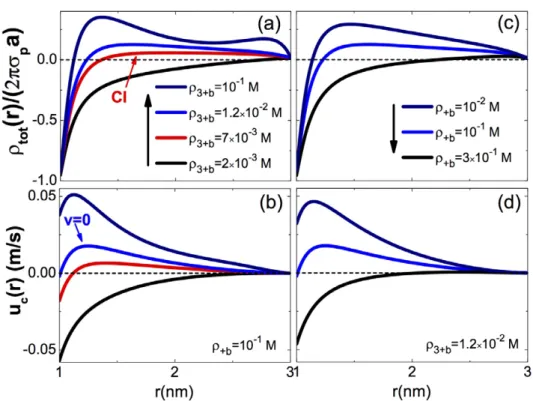
In order to explain the reversal of DNA mobility by mul-tivalent counter-ions, in figure 5(a) we plot the cumulative charge density of the KCl + Spm Cl3+
3 fluid including the
polyelectrolyte charge
∫
ρ r =2π dr r′ ′ρ r′ +σ r′ a r c s tot( ) [ ( ) ( )] (44)for various bulk Spd3+ concentrations. In figure 5(b), we also
illustrate the cumulative liquid velocity (42) at the same den-sities. At the low Spd3+ density ρ = ×
+b 2 10−
3 3 M, moving
from the DNA surface towards the pore wall, the total charge density rises from the net DNA charge towards zero. This corresponds qualitatively to the MFpicture where counter -ions gradually screen the DNA charge. Hence, the negatively charged fluid and DNA move in an opposite way to the field, that is uc(r) < 0 and v = uc(a) < 0. Increasing now the Spd3+
density to ρ + = ×7 10− b
3 3 M, the cumulative charge density
switches from negative to positive at r 1.3 nm. This is the signature of charge reversal, where due to correlation effects induced by Spd3+ ions, counter-ions locally overcompensate
the DNA charge. Consequently, the liquid flows parallel
with the field (uc(r) > 0) in the region r > 1.3 nm. However,
because the hydrodynamic drag force is not sufficiently strong to dominate the electrostatic coupling between the DNA mol-ecule and the external electric field, the molmol-ecule and the liq-uid around it continue to move in the direction of the field. At the higher Spd3+ density ρ = ×
+b 1.2 10−
3 2 M, where charge
reversal becomes more pronounced, the drag force compen-sates for the electric force on the DNA molecule exactly. As a result, the DNA stops its translocation, i.e. v = uc (a) = 0.
At higher Spd3+ concentrations, the DNA molecule and the
electrolyte move parallel with the field. We emphasize that an important challenge in DNA translocation consists of the extremization of the DNA translation velocity for an accurate sequencing of its genetic code [26]. The present result sug-gests that this can be achieved by tuning the trivalent or quad-rivalent ion densities in the liquid.
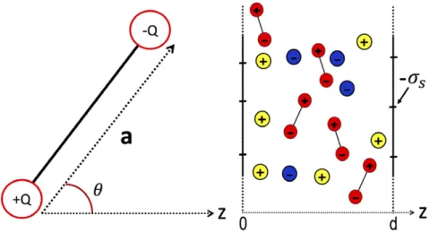
Figure 3. Nanopore geometry: a cylindrical polyelectrolyte of radius a = 1 nm, surface charge −σp, and dielectric permittivity εp is
confined to a cylindrical pore of radius d = 3 nm, with wall charge −σm, and membrane permittivity εm. The permittivity of the electrolyte is ε = 80w .
Figure 4. Polymer translocation velocity against the density of the
multivalent counter-ion species Im+ (see legend) in the electrolyte mixture KCl + IClm. The K+ density is fixed at ρ =+b 0.1 M. The confined double-stranded DNA has a surface charge of σ = 0.4p e nm−2. The potential gradient is ∆ =V 120 mV. Circles mark the charge inversion (CI) point of the DNA molecule.
To summarize, it is found that the inversion of DNA mobil-ity is induced by charge reversal. However, charge inversion should also be strong enough for mobility reversal to occur. This can also be seen in figure 4 where we display the charge inversion points with open circles. One notes that charge inversion precedes the mobility reversal that occurs only with trivalent and quadrivalent ions. We now focus on the peak of the velocity curves in this figure. One notes that at the highest
+
Spd3 concentration in figure 5(a), the first positive peak of the
cumulant charge density is followed by a well. The corresp-onding local drop of the cumulative charge density stems from the attraction of Cl− ions towards the charge-inverted DNA. At
higher Spd3+ concentrations, the stronger chloride attraction
attenuates the charge reversal effect responsible for mobility inversion. This explains the reduction of the inverted charge mobility at high multivalent densities in figure 4. Finally, we consider the effect of potassium concentration that can easily be tuned in translocation experiments. In figures 5(c) and (d), we show the charge density and velocity at a fixed Spd3+
concen-tration for various K+ densities. Starting at the charge-inverted
density values ρ + =1.2×10− b
3 2 M and ρ =+b 10−2 M,
and raising the bulk potassium concentration from top to bot-tom, the cumulative charge density is seen to switch from positive to negative. This drives the DNA and electrolyte velocities from positive to negative. Thus, the K+ ions cancel
the DNA mobility inversion by weakening the charge reversal effect induced by ion correlations.
In the next paragraph, we will discuss the effect of charge reversal on the ion currents induced by a pressure gradient.
3.1.3. Inversion of hydrodynamically induced ion currents through nanopores. We now investigate the effect of charge correlations on streaming currents during hydrodynami-cally-induced polymer translocation events [11]. The DNA- membrane geometry, including the electrolyte mixture, is the same as in the previous section. The only difference is that in hydrodynamically-induced transport experiments, the exter-nally applied voltage difference in figure 3 is replaced with a pressure gradient ∆ >Pz 0 at the pore edges. The resulting
ionic current through the nanopore of length L = 340 nm and radius d = 3 nm is given by the number of charges flowing per unit time through the cross section of the channel,
( ) ( )
∫
π ρ = ∗ ∗ I 2 e drr r u r . a d c s str (45)In equation (45), we introduced the effective pore and poly-mer radii d∗= −d a
st and a∗= −a ast where ast=2Å stands
for the Stern layer accounting for the stagnant ion layer in the vicinity of the charged pore and DNA surfaces. The charge density function ρ rc( ) is defined by equation (38). The stream-ing current velocity is given in turn by the solution of the Stokes equation with an applied pressure gradient
( )
η∆u r +∆P =
L 0.
s z
(46)
Solving equation (46), we impose the boundary conditions
( ) =∗
u ds 0 (no-slip) and u as( ) =∗ v. We also account for the fact that the viscous friction force F=2π ηa u a∗ ′ ∗
v s( ) vanishes in the stationary state of the flow. Integrating equation (46)
Figure 5. Cumulative charge densities rescaled with the bare DNA charge (top plots) and solvent velocities (bottom plots) at a fixed K+
and a varying Spd3+ concentration in (a) and (b), and a fixed Spd3+ and a varying K+ concentration in (c) and (d). In each column, the same colour in the top and bottom plots corresponds to a given bulk counter-ion concentration displayed in the legend. The remaining parameters are the same as in figure 4.
under these conditions, the streaming flow velocity follows in the form of a Poisseuille profile,
( ) ⎡ ⎜ ⎟ ⎣⎢ ⎛⎝ ⎞⎠⎤⎦⎥ η =∆ ∗ − + ∗ ∗ u r P L d r a r d 4 2 ln . s z 2 2 2 (47)
Knowledge of the charge density (38) and liquid velocity (47) completes the calculation of the ionic current of equation (45).
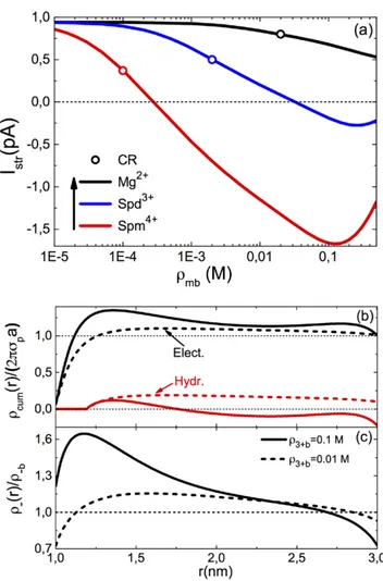
In figure 6(a), we report the streaming currents of the elec-trolyte mixture KCl+IClm against the reservoir density of the multivalent cation species Im+ in a neutral pore. At weak
mul-tivalent ion densities the current is positive. This corresponds to the MF-regime where the negatively charged translocating DNA attracts cations into the pore. Increasing the bulk mag-nesium concentration in the KCl+MgCl2 liquid, in agree-ment with the MF ion transport picture, the streaming current drops slightly but remains positive. However, in the liquids containing spermidine and spermine ions, at a characteristic multivalent ion density, the current turns from positive to neg-ative. It is noteworthy that this streaming current reversal has been previously observed in nanofluidic transport experiments through charged nanoslits without DNA [27].
The positive ion currents of figure 6(a), indicating a net negative charge flow through the pore, cannot be explained by MF-transport theory. In order to explain the underlying mechanism behind the current reversal, in fig-ure 6(b) we plot the electrostatic cumulative charge density
∫
ρ r =2π dr r′ ′ρ r′
a r
c
cum( ) ( ) and the hydrodynamic cumulative
charge density ρ∗ r =2π
∫
a∗dr r′ ′ρ r′r c
cum( ) ( ) of the KCl+SpdCl3
liquid normalized by the DNA charge. The hydrodynamic charge density only accounts for the mobile charges contrib-uting to the streaming flow. Figure 6(c) displays the chloride densities between the DNA and pore surfaces. At the bulk sper-midine concentration ρ3+b=0.01 M, figure 6(b) shows that the electrostatic cumulative charge density slightly exceeds the DNA charge. This is the sign of a DNA charge reversal effect. This in turn leads to a weak Cl− excess ρ( )>ρ
−r −b
between the pore and the DNA (see figure 6(c)). However, because the charge reversal and the resulting chloride attrac-tion is weak, the hydrodynamic flow charge dominated by the counter-ions is positive, i.e. ρ∗ >0
cum for a∗< <r d∗. With an
increase of the spermidine density to ρ3+b=0.1 M, where one arrives at the inverted current regime in figure 6(a), the intensified DNA charge reversal results in a much stronger Cl−
attraction into the pore (see figures 6(b) and (c)). This strong anion excess leads in turn to a negative hydrodynamic charge density ρcum( )d <0 and a negative streaming current through the pore.
To conclude, these calculations show that ionic current inversion during hydrodynamically induced DNA transloca-tion events results from the anion excess in the pore induced in turn by the DNA charge reversal. It is important to note that, similar to the electrophoretic DNA transport of the previous section, the observation of streaming current reversal neces-sitates a strong DNA charge inversion for the adsorbed ani-ons to bring the dominant contribution to the hydrodynamic flow. This is again illustrated in figure 6(a) where the charge
reversal densities (open circles) are seen to be lower than the current inversion densities by several factors.
3.2. Solving SC equations in dielectrically inhomogeneous systems
In the previous paragraphs, we have considered the conse-quences of the charge reversal effect in different settings. In the next section, we will focus on the image-charge effects in dielectrically inhomogeneous systems.
3.2.1. Inversion scheme for the solution of the SC equa-tions. In this section we present the solution of the SC equa-tions (10) and (11) in dielectrically inhomogeneous systems. The technical details of the solution scheme that can be found in [6, 7] will be briefly explained for the case of neutral inter-faces. In this case, where the average potential ψ r( ) is zero, the fluctuation-enhanced Poisson–Boltzmann equation (10)
Figure 6. (a) Streaming current curves at a pressure gradient
∆ =Pz 1 bar against the reservoir density of the multivalent
counter-ion species listed in the legend. Open circles mark the DNA charge reversal (CR) points. (b) Electrostatic (black curves) and hydrodynamic (red curves) cumulative charge densities, and (c) Cl− densities in the KCl+SpdCl3 liquid at the reservoir concentrations ρ3+b=0.01 M (dashed curves) and 0.1 M (solid curves). The
neutral nanopore (σ = 0m ) contains a double-stranded DNA molecule of charge density σ = 0.4p e nm−2, with a bulk K+ density
vanishes. This leaves us with equation (11) to be solved in order to evaluate the ion density
( ) ( ) ρ r =ρ e− δ , i b q vr 2 2 (48) with the ionic self-energy δv r( ) defined by equation (12). The iterative solution strategy consists of recasting the differential equation (11) in the form of an integral equation. To this end, we re-express equation (14) as [ ] ( ) ( ) ( ) ( ) ( ) κ π δ π δ ∇ − = − − = − ′ ′ ′ − v n v r r r r r r r e , 4 4 , b V r 2 2 B B w (49) where we defined the number-density correction function
( ) ( )⎡ ( ) ⎣⎢ ⎤ ⎦⎥ δn r =2q ρ e− 1−e− δ . b V q v r r 2 w 2 2 (50)
Introducing now the DH-kernel
π κ δ = − ∇ − − ′ ′ − − v r r, 1 r r 4 be V r 01 B 2 2 w ( ) { ( )} ( ) (51) and using the definition of the Green’s function (16), one can invert equation (49) and finally obtain
( ′)= ( ′)+
∫
″ ( ″) ( ) (δ ″ ″ ′) vr r, v0r r, dr v0 r r, n r vr r, .(52) Equation (52) expresses the solution of the SC-kernel equa-tion (11) as the sum of the Debye–Hückel potential v0(r r, )′
solution to equation (49) and a correction term associated with the non-uniform charge screening induced by image-charge forces. The iterative solution scheme of equation (52) con-sists of replacing the potential v(r r, )′ on the rhs with the DH potential v0(r r, )′ at the first iterative step, inserting the output
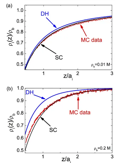
potential v(r r, )′ into the rhs of the equation at the next iterative level, and continuing this cycle until numerical conv ergence is achieved. The solution scheme for charged interfaces/nano-pores is based on the same inversion idea but technically more involved. The more general scheme can be found in [6, 7]. 3.2.2. Image-charge-induced correlations at planar inter-faces. In figure 7, we display the monovalent ion density profiles obtained from the DH and the SC theories that we compare with MC simulations [6]. The dielectric interface located at z = 0 is neutral and the membrane permittivity is ε = 1m . We emphasize that this configuration is also relevant to the water–air interface, whose surface tension was first cal-culated by Onsager and Samaras [28]. Because their calcul-ation was based on the uniform screening approx imcalcul-ation corresponding in our case to the DH approach, the latter is called the Onsager approximation as well. The separation distance is rescaled by the ion size ai, introduced in order to
stabilize the MC simulations. At the salt density ρ = 0.01b M (top plot), the SC result exhibits a very good agreement with the MC simulations while the DH-theory slightly deviates from the MC data, although the error is minor. At this bulk salt concentration where the electrostatic coupling parameter
κ
Γ = b B≈0.2 corresponds to the weak-coupling regime, the
accuracy of the DH-theory is expected. At the much higher salt density ρ = 0.2b M (bottom plot), the SC-theory exhibits
a good agreement with the MC data but the DH-result overes-timates the ion density over the whole interfacial regime.
The inaccuracy of the DH-result is due to the fact that the ion density ρ = 0.2b M corresponds to the intermediate coupling regime Γ ≈ 1. The overestimation of the ion density stems from the non-uniform salt screening of the image-charge potential at the interface. The mobile ions that screen this potential also being subject to image-charge forces, the interfacial charge screening is lower than the bulk screening. As the DH-theory assumes a con-stant screening parameter κb, it cannot account for the reduced screening at the interface. In the SC-theory, this effect is taken into account by the second term on the rhs of equation (52), correct-ing the uniform screencorrect-ing approximation of the DH-theory. We also note that in the close vicinity of the interface, the SC-theory slightly deviates from the MC result. This may be due to ionic hard-core effects neglected so far in the SC-formalism. The weak deviation of the SC theory from the MC data is likely to result from excluded volume effects related to ion size but absent in the SC theory. Although the inclusion of ion size is still an open issue, the excluded volume effects can be included into the pre-sent SC theory via repulsive Yukawa interactions (see e.g. [24]).
Figure 7. Ion density profiles at the dielectric interface against the
distance from the surface with ε = 1m , ε = 80w , and ion diameter ai = 4.25 Å at the bulk ion concentration (a) ρ = 0.01b M and (b)
ρ = 0.2b M. The red lines are MC simulation data, the blue lines the DH theory, and the black lines are from the SC scheme (52). The theoretical curves and MC data are from [6].
3.2.3. Image-charge effects on ion transport through α-Hemolysin pores. The most significant implication of image-charge correlations is found in electrophoretic image-charge transport through strongly confined α-hemolysin pores. The particularly
low conductivity of these pores cannot be explained by MF elec-trophoresis. As in the previous section, we will model the pore as a neutral cylinder with a radius of d = 8.5 Å and a length of L = 10 nm [26] (see figure 3). In the most general case, the pore may be blocked by a single-stranded DNA molecule with a radius of a = 5.0 Å [26]. The pore also contains the monovalent electrolyte solution KCl. Under an external potential gradient
∆V, the total velocity of the positive or negative ionic species
( )= ( )+ ( )
± ±
u r u rc uT r is composed of the convective velocity
uc(r) given by equation (44), and the drift velocity
µ = ± ∆ ± ± u r V L , T ( ) (53) where µ± stands for the ionic mobility. The ionic current is given by ( ) ( )
∫
∑
π ρ = =± I 2 e q drr r u r . i i a d i i (54)Inserting the total velocity u(r) and the ion number density
( )
ρ ri into equation (54), the conductivity takes the form of a linear response relation I= ∆G V, where G stands for pore conductance (see [10] for its functional form).
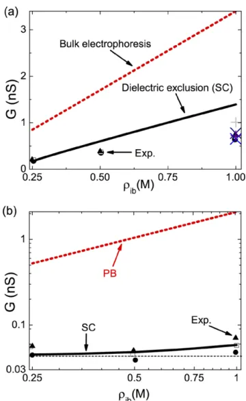
In figure 8(a), we illustrate the conductance of a DNA-free
α-hemolysin pore against the reservoir salt density. It is seen
that the classical bulk conductivity G=π ρ µe ib( ++µ−) /d L2
overestimates the experimental conductance data by an order of magnitude. However, the SC-theory that can account for image-charge interactions lowers the MF-theory to the order of magnitude of experimental data, with a quantitative agree-ment at low ion densities and a qualitative agreeagree-ment at high concentrations. The weak pore conductivity is induced by image-charge interactions between the low permittivity mem-brane and the nanopore. The radius of these pores being com-parable with the Bjerrum length d≈ B, this results in strongly
repulsive polarization forces excluding ions from the pore medium and reducing the net conductance.
Figure 8(b) displays the conductance of the same α-hemolysin
pore blocked now by the single-stranded DNA (see caption for the characteristic parameters of the DNA molecule). One notes that unlike the conductance of DNA-free pores exhibiting a lin-ear increase with the salt density, the blocked pore conductance rises non-linearly at high densities but weakly changes with salt at dilute concentrations. As the PB-conductivity increases lin-early with salt density (dashed red curve), the non-linear behav-iour of the blocked pore conductivity is clearly a non-MF effect. One also notes that the SC theory can reproduce the non-linear shape of the exper imental conductivity data accurately.
In [10], it is shown that the low density conductance of the blocked pore is given by
π µ σ = + G e L a 2 . p (55) The limiting law (55) is displayed in figure 8(b) by the dashed horizontal curve. This law is independent of the salt
concentration and depends only on the mobility of counter-ions. Indeed, this counter-ion-driven charge conductivity results from the competition between repulsive image-charge interactions and attractive DNA-counter-ion interactions driven by the pore’s electro-neutrality. More precisely, as one lowers the bulk ion density, image-charge forces strongly excluding the ions cannot lead to a total ionic rejection, since a minimum number of ions should stay inside the pore in order to screen the DNA charge. In the dilute concentration regime of figure 8(b), these counter-ions contribute solely to the pore conductance. Hence, the low density limit of pore conductance corresponds to a non-MF counter-ion regime, whose density is fixed by the DNA surface charge rather than
Figure 8. (a) Conductivity of an α-hemolysin pore against the
reservoir concentration of the KCl solution. The pore, modelled as an overall neutral cylinder (σ = 0.0m C m−2), has a radius of d = 8.5 Å and a length of L = 10 nm. Experimental data: black circles, triangles, and open squares from figure 2 of [26], and the additional data at the bulk ion density ρ = 1.0ib M from [29] (plus symbol) and table 1 of [30] (cross symbols). (b) The pore in (a) is blocked by a single-stranded DNA molecule with a radius of a = 5.0 Å [26] and a dielectric permittivity of ε = 50p . The effective smeared charge distribution of the ss-DNA is fixed to a value σ = 0.012p e nm−2 providing the best fit with the experimental data (symbols) taken from figure 3 of [26].
the bulk ion density. At high bulk ion densities, the chemical equilibrium between the pore and bulk media takes over. As a result, co-ions penetrate into the pore and the conductance starts rising with the bulk salt density.
This discussion concludes section 3 of the review, covering the solutions of the self-consistent equations for systems with continuum dielectric properties. In the subsequent section, we turn to the effects of charge correlations in solvent-explicit electrolyte models.
4. The dipolar Poisson–Boltzmann equation
In the previous section we have developed a theoretical treat-ment of current soft matter problems in which the solvent structure is modelled sufficiently well by the assumption of continuous dielectric media—in particular of the solvent— and hence can be described in terms of a dielectric constant. This description is one of scale: if one has to consider systems on molecular scales, this assumption becomes questionable. There has, therefore, been recent interest in including sol-vent properties more explicitly with the Poisson–Boltzmann theory, and one such example is the family of models which include, as a first step, solvent properties in the form of molec-ular dipoles. This is done first within the point dipole limit, which allows the formulation local to be kept local. The prop-erties of these theories within mean-field treatments and their application to protein electrostatics have been discussed in a series of papers in recent years [12, 13, 31–38], see also the review [39].
4.1. Self-consistent equations for point-dipoles and ions Here, we derive the variational equations for ions in a point-dipole solvent. The liquid is assumed to be in contact with charged slit membrane walls, though the formulation is valid in all geometries. The solvent geometry and the fluid configu-ration is shown for slit membranes in figure 7. As the self-consistent equations derived here are novel, we present the derivation in detail.
The grand canonical partition function of ions and dipolar solvent molecules in contact with fixed charge distributions is given by the functional integral over potential configurations
[ ]
∫
φ= − φ
ZG D e H [12, 13], with the Hamiltonian
[ ] [ ( )] ( ) ( ) ( ) ( ) ( ) ( )
∫
∫
∫
∑
φ φ π σ φ π Ω = ∇ − − Λ − Λ φ φ − + ⋅∇ − + ⎡ ⎣⎢ ⎤ ⎦⎥ H r i r r r r r r d 8 d d 4 e d e s V i i i V iq r p r r 2 B s i i (56)where we introduced the dipole moment p= −Qa, and dipo-lar and ionic wall potentials Vs( )r and Vi( )r. In equation (56), the first integral term accounts for the electrostatic energy of freely propagating waves in a vacuum. It is important to note that the Bjerrum length in a vacuum B=e2/(4πε0 Bk T) differs
from the one used in the previous chapter for the dielectric continuum model: the dielectric constant of water is absent, as the dipoles explicitly model water properties. The second term of equation (56) is the contribution from solvent molecules
modelled as point dipoles with fugacity Λs. Finally, the third term is due to the mobile ions with fugacity Λi. As stated in the introduction, the SC equations can be derived from a varia-tional extremization principle. The grand potential to be mini-mized has the form [3]
Ω = Ω +v 0 H−H0 0,
(57) where the bracket ⋅ 0 denotes the field-theoretic average with respect to the quadratic reference Hamiltonian of the form of equation (2), [ ( ) ( )] ( )[ ( ) ( )]
∫
φ ψ φ ψ = − − ′ ′ − ′ ′ H 1 r r v r r r r 2 r r , . 0 , 1 (58)In equation (58), we introduced the trial external potential
( )
ψ r and the electrostatic kernel v−1(r r, ′). First, we note that in
equation (57), the part of the grand potential corresp onding to the Gaussian fluctuations of the electrostatic potential is given by Ω = −0 Tr ln[ ]/v 2. Evaluating the field-theoretic averages
in equation (57), one obtains the variational grand potential in the form of the following fairly involved expression
∫
∫
∫
∫
∫
∑
∫ ∫ π ψ σ ψ π δ π Ω Ω = − + ∇ − + − ∇ ⋅ ∇ − Λ −Λ ′ ′ ′ ′ ψ δ ψ δ − + − − − + ⋅∇ − − ⋅∇ ⋅∇ ′ ′ ′ ′ ′ ′ ′ v v r r r r r r r r r r r r r 1 2Tr ln d 8 i d d d 8 , d e d d 4 e . v i i V q q v s V v r r r r r r r r r r p r r r r p p r r B 2 B i 2 d , i 12 d , i i s r r r i 2 [ ] [ ( )] ( ) ( ) ( ) ( ) ( ) ( ) ( ) ( ) ( ) ( ) ( )( )( ) ( ) (59) The ionic and solvent number densities follow from the thermo-dynamic relations ρi( )r = Ω Vδ v/ ( )δ i r and ρs( )r = Ω Vδ v/ ( )δ sr. One finds ( ) ( ) ( ) ( ) ρir = Λie−V −qψ − q v r r 2 r r, i i i 2 (60)∫
∫
ρ π Ω = Λ − + ⋅∇ψ − ′δ − ′ ⋅∇ ⋅∇ ′ ′ r d 4 e . s s V r ip r r r r p p vr r 1 2 d , s r r r ( ) ( ) ( ) ( )( )( ) ( ) (61) In the bulk region, where the electrostatic potential vanishes,( ) →
ψ r 0, and the propagator satisfies spherical symmetry,
( ′) → ( − ′)
vr r, vbr r , from equations (60) and (61) one gets the relation between the bulk densities and fugacities as
( ) ρ = Λ e− − i q v r r ib 2 i b 2 (62)
∫
ρ = Λse− r r r p′δ − ′ ⋅∇ p⋅∇′v r r− ′. sb 1 2 d ( )( r)( r) (b ) (63) Passing from equations (60)–(63), we accounted for the fact that in the bulk region, the dipolar potential of mean force (PMF) in the exponential is independent of the dipolar orientation.The SC equations follow from the optimization of the variational grand potential with respect to the electrostatic potential ψ r( ) and propagator v(r r, ′), i.e. δΩv/ ( )δψ r =0 and
/ ( )
δΩvδvr r, ′ =0. By evaluating the functional derivatives and