Modeling the supplier uncertainty with phase-type distributions in inventory problems

? 1 іі^ггі- ΐ ί Τ Φ ^ ν S »·<* i » w ij w - M. w.í> ., w ^ -:.^·^ 3 ^ Ъ ^ le; w Ь v'<* ;' ;. j ^ ^vi ¡j -J^ ¿‘-^ y

2-?Л!ТГН2- ТО THE DEPAHTMEfvT OF fMD4.í81T¡ÍAL ННві^.?ЕЕ5ТШ wir '¿Ü * β*« j*i " .W ^ O Q í? »T'c: :^:T ÜtİÎVSHSîT / 'r- tr:^’:'·· ξ ^f*w'ц ѵ^ Г* *r ’“î'T t:···'Г’·' О«- ^Г;w r^::''w.w/^:rv^4v.w«·' - WW· f O B THE DEOPE-E Z: 'u /Л S*·· '-‘ р·'’"'' -■ '-'Л'-С г і ' τ· ·:ι :· 'чі5 «Λ’ І ч^ѵ j;i .· · .-.есг i V iC^

MODELING THE SUPPLIER UNCERTAINTY WITH

PHASE-TYPE DISTRIBUTIONS IN INVENTORY

PROBLEMS

A THESIS

SUBMITTED TO THE DEPARTMENT OF INDUSTRIAL ENGINEERING

AND THE INSTITUTE OF ENGINEERING AND SCIENCES OF BILKENT UNIVERSITY

IN PARTIAL FULFILLMENT OF THE REQUIREMENTS FOR THE DEGREE OF

MASTER OF SCIENCE

By

Ahmet Barış Balcıoğiıı

September, 1996

İ5%

11

I certify that I have read this thesis and that in my opinion it is fully adequate, in scope and in quality, as a thesis for the degree of Master of Science.

' k

(Principal Advisor) Assoc. Prof.Nulku

I certify that I have read this thesis and that in my opinion it is fully adequate, in scope and in quality, as a thesis for the degree of Master of Science.

I certify th at I have read this thesis and that in my opinion it is fully adequate, in scope and in quality, as a thesis for the degree of Master of Science.

Assist. Prof. Refik Güllü

.Approved for the Institute of Engineering and Sciences:

/

-Prof." Mehmet B a r ^

MODELING THE SUPPLIER UNCERTAINTY WITH

PHASE-TYPE DISTRIBUTIONS IN INVENTORY

PROBLEMS

Ahmet Barış Balcioglii

M.S. in Industrial Engineering

Supervisor: Assoc. Prof. Ülkü Gürler

September, 1996

This study considers a stochastic inventory nnodel where the supply availability is subject to random fluctuations. The periods in which the supplier is available (ON) or unavailable (OFF) are modeled as a semi-Markov process. During ON periods the {q,r) policy is applied. During OFF periods, the amount enough to bring the inventory position to q + r is ordered as soon as the supplier becomes available again. The regenerative cycles are identifled by observing the inventory position and using the renewal reward theorem the average cost per time objective function is derived. In our study, a K-stage Phase-Type distribution for ON periods and a general distribution for OFF periods are assumed. In our study, the problem is theoretically solved for K- stage Phase-Type distributions; additionally numerical computations are made for 2-stage Phase-Type distributions. For large q values the structure of the objective function is investigated.

Key words: Inventory Models, Phase-Type Distribution, Semi-Markov

Processes, Supplier Availability

ÖZET

ENVANTER PROBLEMLERİNDE SUNUCUNUN

BELİRSİZLİĞİNİN EVRE-TÜRÜ DAĞLIMLARLA

MODELLENMESİ

Ahmet Barış Balcıoğlıı

Endüstri Mühendisliği Bölümü Yüksek Lisans

Tez Yöneticisi: Doç. Ülkü Gürler

Eylül, 1996

Bu çalışmada çeşitli nedenlerden ötürü arzın rassal dalgalanmalar gösterdiği l)ir envanter modeli anlatılmaktadır. Sunucunun hizmet verdiği (AÇIK) ve veremediği (KAPALI) süreler bir yarı-Markov süreç olarak modellenmiştir. AÇIK durum larda {q,r) politikası uygulanmaktadır. KAPALI durumda ise sunucu tekrar çalışabilir duruma gelince, envanter pozisyonunun q + r'ye çıkması için yetecek m iktarda ısmarlama yapılır. Yeniden tekrarlanabilir çevrimler, envanter pozisyonu gözlemlenerek belirlenir ve yenileme ödül kuramı kullanılarak birim zaman ortalama maliyet işlevi türetilir. Çalışmamızda, AÇIK dönemler için K- aşamalı Evre- Türü, KAPALI dönemler içinse genel bir dağılım varsayılmaktadır. Bu çalışmada, problem K-aşamalı Evre-Türü dağılım için kuramsal olarak çözülmüş, ayrıca 2-aşamalı Evre-Türü dağılımlar kullanılarak sayısal çözümlemelere gidilmiştir. Büyük q değerleri için amaç işlevinin yapısı da incelenmiştir.

Anahtar sözcükler. Envanter Modelleri, Evre-Türü dağılımlar, Yarı-Markov

To my family

ACKNOWLEDGEMENT

I am mostly grateful to Ülkü Gürler for suggesting this interesting research topic, and who has been supervising me with patience and everlasting interest and being helpful in any way during my graduate studies.

I am also indebted to Refik Güllü and Halim Doğrusöz for showing keen interest to the subject m atter and accepting to read and review this thesis. I'heir remarks and recommendations have been invaluable.

I would like to thank to Mahmut Parlar who has not only aided me with his valuable suggestions but with his computer program th at I revised, as I would be unlikely to complete the required numerical analysis otherwise.

I have to e.xpress my gratitude to the technical and academical staff of Bilkent University. I am especially thankful to my classmates of my first graduate year, and my office mates, especially Muhittin Demir for helping me in any way during the entire period of my M.S. studies. I can not forget the aids of Hakan Ozaktaş who always supported me with my m aster’s thesis.

Finally I have to e.xpress my sincere gratitude to anyone who have been of help, which I have forgotten to mention here.

1 In trod u ction and Literature R ev iew 1 1.1 Literature R eview ... 4

2 P h a se-T y p e D istribution s 9 2.1 Definitions and Closure P r o p e r tie s ... 11

2.1.1 Discrete Phase-Type Distributions 14

2.1.2 Closure Properties 1,5

2.2 Special PH-Type D is trib u tio n s ... 17 2.2.1 Mixtures of Generalized Erlang (Coxian) Distributions

(M G E )... 17 2.2.2 Hyperexponential D istrib u tio n ... 19 2.3 Equivalence Relations Between Some Classes of PH-Type

Distributions 20

2.3.1 Exponential and Arbitrary Phase-type Distributions . . . 20 2.3.2 Hyperexponential and MGE D is trib u tio n s ... 20

2.4 Moment Approximations 23

2.4.1 Three-moment approximations (c > 1 ) ... 23

2.4.2 Two moment ap p ro x im atio n ... 26

3 T he M od el and N otation s 28 3.1 The Semi-Markov Processes and The Objective Function . . . . 30

3.1.1 Cycle L e n g t h ... 30

3.1.2 Cycle C o s t... 32

3.1.3 Computation of E[N(q)] 36 3.2 Integral Equations of The Transition P ro b ab ilities... 37

3.2.1 Transient Solutions of Pij(t) for special Phase-type d istrib u tio n s... 38

4 A n alytical R esu lts 41 4.1 Analysis of 2-stage Coxian d is tr ib u tio n ... 41

4.2 Analysis of The Model for Large q ... 45

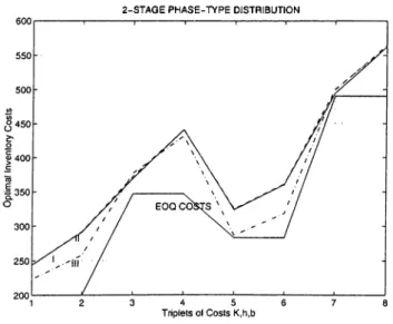
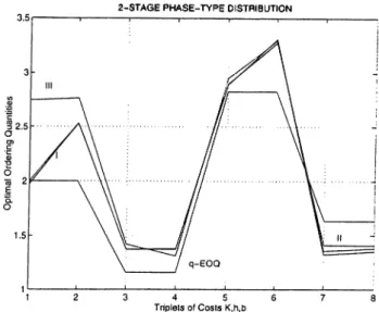
4.2.1 The Limiting Probabilities of Phase-Type Distributions . 46 5 N u m erical R esu lts 52 5.1 2-Stage Phase-Type Distribution 53 5.1.1 Moments of ON and OFF p e rio d s ... 53

5.1.2 General C a s e ... 54

5.1.3 Special C a s e ... 57

5.2 2-Stage Coxian D is trib u tio n ... 62

5.3 Comparison of .Several Phase-Type D istributions... 65

6 C onclusion 75

A Som e C om p utational Issues 77

B C om p u ter Program 81

B IB L IO G R A P H Y 109

List of Figures

2.1 Coxian distribution with m phases ₁₀

2.2 Phase-type distribution with m phases... 11

2.3 Graphical representation of MGE d is tr ib u tio n ... 18

2.4 Graphical representation of the Erlang d is t r ib u t i o n ... 19

2.5 Graphical representation of the hyperexponential distribution 19 2.6 Weighted Hyperexponential distribution 2i 3.1 Regenerative Cycles of the Inventory Position 29 3.2 Phase-type distribution with k phases. 30 3.3 Graphical representation of the Erlang d is t r ib u t i o n ... 39

3.4 Graphical representation of the Coxian d is tr ib u tio n ... 40

4.1 2-Stage Coxian D is trib u tio n ... 41

4.2 k-Stage Phase-Type Distribution ... 47

4.3 k-Stage Coxian D is trib u tio n ... 48

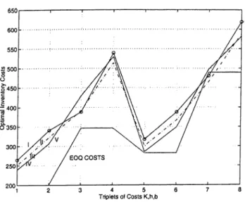
5.1 Comparison of Optimal Costs ( 1 ) ... 57 XI

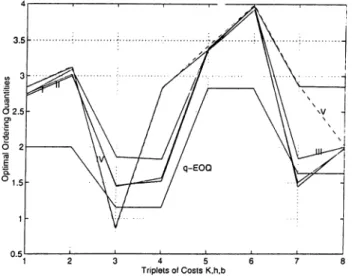
5.2 Comparison of Optimal ( 1 ) ... 58

5.3 Comparison of Optimal Costs ( 2 ) ... 61

5.4 Comparison of Optimal qs { 2 ) ... 62

5.5 Comparison of Optimal Costs ( 3 ) ... 65

5.6 Comparison of Optimal ( 3 ) ... 66 5.7 When K=200, h=100, b=500 ... 67 5.8 When K=200, h=100, b=1000 ... 67 5.9 When K=200, h=300, b=.500 68 5.10 When K=200, h=300, b=1000 ... 68 5.11 When K=400, h=100, b=500 69 5.12 When K=400, h=100, b=1000 ... 69 5.13 When K=400, h=300, b=500 70 5.14 When K=400, h=300, b=1000 ... 70 5.15 When K=200, h=100, b=500 71 5.16 When K=200, h=100, b=1000 ... 71 5.17 When K=200, h=300, b=500 ... 72 5.18 When K=200, h=300, b=1000 ... 72 5.19 When K=400, h=100, b=500 73 5.20 When K=400, h=100, b=1000 ... 73 5.21 When K=400, h=300, b=500 ... 74

LIST OF FIGURES Xlll

5.1 Sensitivity Analysis When Coi=0.5, Co2=0.5 E[ON]=3.6667, Var[ON]=13.518.3... 55 5.2 Sensitivity Analysis When coi=0.4, Co2=0.6 E[ON]=3.68S9,

Var[OM] = 13.5722 ... 56 5.3 Sensitivity Analysis When Coi=0.3, Co2=0.7 E[ON]=3.7111,

Var[ON]=13.6252 ... 56 5.4 Sensitivity Analysis When Aj=0.4, A2=0.5 E[ON]=4.5000,

V ar[O N ]= 1 0 .2 5 ... .58 5.5 Sensitivity Analysis When Ax =0.5, A2=0.4 E[ON] =4.5000,

V ar[O N ]= 1 0 .2 5 ... 59 5.6 Sensitivity Analysis When Ai=0.5, A2=0.5 E[ON]=4.0000,

Var[ON]=8 60

5.7 Sensitivity Analysis When Ax =0.6, A2=0.5 E[ON] =3.6667, Var[ON]=6.7775 ... 60 5.8 Sensitivity Analysis When Ax=0.5, A2=0.6 E[ON]=3.6667,

Var[ON]=6.7775 ... 61 5.9 Sensitivity analysis when ax = 0.0 E[ON]=1.6667, Var[ON]=2.7777 62 5.10 Sensitivity Analysis When ax= 0.1 E[ON]=1.8667, Var[ON]=3.5376 63

LIST OF TABLES X V

5.11 Sensitivity Analysis When a i= 0.2 E[ON]=2.0667, Var[ON]=4.2176 6.3 5.12 Sensitivit}'^ Analysis When a i= 0.3 E[ON]=2.2667, Var[ON]=4.8176 63 5.13 Sensitivity Analysis When a i= 0.6 E[ON]=2.8667, Var[ON]=6.1376 64 5.14 Sensitivity Analysis When a i= 1.0 E[ON]=3.6667, Var[ON]=6.7775 64

Introduction and Literature

Review

Inventory problems are as old as human history, but introduction of analytical tools to study these problems has started since the beginning of this century. The importance of studying inventory problems arises from the fact that, we can not avoid carrying inventories due to several reasons, the main one being that it is either physically or economically impossible to obtain and distribute goods whenever demand occurs. If inventories are not kept then the customers should wait until their orders are supplied which will result in low customer satisfaction. Other than this, to cope with the effects of inflational or seasonal fluctuations of demand and prices, manufacturers are forced to hold inventories. Several other reasons may be listed similarly.

The basic questions that inventory managers are faced with are:

• How often should the inventory status be checked (i.e. what should be the review interval)?

• When to replenish the inventory? • How much to order for replenishment?

These issues are handled by introducing mathematical models for inventory processes. A good mathematical model should capture the main features of the real problem, while avoiding analytical and numerical complexities. Inventory systems differ in size and complexity, in the types and nature of the items they carry, in the nature of information available to decision makers, in the costs related with operating systems. Most of the inventory models aim to minimize an objective function with respect to costs, although there may be other objectives such as profit maximization etc. Basically four types of costs relevant to an inventory problem:

(i) R ep len ish m en t Costs

This is the cost incurred each time a replenishment action is taken. It can be considered in two parts: (i) the fixed amount, often called setup or ordering cost, which must be paid to the source independent of order size, (ii) a component th at depends on the size of the replenishment.

(ii) In ven tory Carrying Costs

Holding stocks include several costs such as: (i) the opportunity cost which is the cost of capital tied up in inventory rather than having it invested elsewhere, (ii) warehouse operation costs, (iii) insurance, (iv) taxes, (v) potential spoilage or obselecence of goods. Usually these costs are accepted to be proportional to the average inventory level, where, in fact some components may be related to inventory level in a more complicated manner.

(iii) Stock ou t C osts

When stocks in hand are insufficient to meet customer demand, costs are incurred as costs of back ordering and/or lost profit on sales other than loosing the good will of the customer due to poor service.

(iv) S y stem C ontrol C osts

It includes the costs of acquiring the data necessary for the adopted decision rules, the computational costs and costs of implementation. However in this sequel this cost type is ignored.

CHAPTER 1. INTRODUCTION AND LITERATURE REVIEW 2

Most of the research that has appeared in the literature implicitly assumes that the goods are available from the supplier at any time an order is

placed. Even in the models which include a (possibly random) lead-time, the assumption is that the supplier will start production of the order and will deliver the amount that has been required as soon as the lead-time ends.

This assumption may be approved only if the supplier is ’always’ available to meet the demand requested. However in practice, supply of the product may be disrupted due to several reasons as discussed below. Therefore, in this study we consider a model where the supplier could also go through ON and OFF times with random durations.

Following examples given by Gürler and Parlar [9] may illustrate the O N /O FF structure of the suppliers: If the supplier has its own inventory process, then we can say that the supplier is ON if ordered quantity q is available in its inventory, and OFF otherwise. Or, as in a frequently encountered example, supplier is considered as a production process which is under statistical process control. The process may start production of items out of specification limits beyond an acceptable proportion and inevitably the process should be stopped before reaching the desired capability. In this case the OFF times of the supplier will be the counterpart of the termination of production while system is being inspected. Similar to this case, machine breakdowns or some maintenance policies may also yield in disruptions in production process and a need for studying supplier unavailability may arise. Rare events such as strikes, embargoes or forced shutdowns of the plants are other possible reasons for disruptions.

When such examples are considered, i.e., in cases when outside supplier may not meet the supply at random times for random durations, the implicit assumption of continuous supply availability would not be valid and new models should be constructed to handle the disruptions of supply.

CHAPTER 1. INTRODUCTION AND LITERATURE REVIEW

1.1

Literature Review

There is a vast literature on modeling inventory problems. It is therefore not attem pted here to give an extensive survey of such studies. The interested reader could refer to Lee and Nahmias [11], Porteus [23], Peterson and Silver [22], Silver [27] and the references therein. Instead, we present below the main studies where supplier unavailability is considered.

Silver [27] is recognized to be the first author who discussed the need of studying supplier unavailability while constructing inventory models. In his review paper, which is also important as it points out the ‘serious gaps existing between the theory and practice in many organizations’. Silver says that while considering the nature of the supply process, most of the literature ignores that ’only a random portion (including 0, perhaps caused by a strike or poor quality conditions) of the ordered material is received’. This is why he suggests finding simple decision rules that must be valid under these circumstances. While explaining the motivation for holding inventories, Nahmias [16] lists three im portant uncertainties that play a major role as (i) uncertainty of external demand, (ii) uncertainty of lead time and (hi) uncertainty of the supply. To make the third one to be understood more clearly, Nahmias gives the OPEC oil embargo of the late 70’s as an example when the electric utilities and the airlines had to cope with curtailing operations due to fuel shortages. Other im portant uncertainties are uncertainty of yield and uncertainty of capacity. We suggest interested reader to read the review article of Yano and Lee [28] on random production and procurement yields.

In order to represent disruptive events such that in our case it is the supplier availability, alternating renewal process models are used. Meyer et

al [14] used this approach while analyzing a single stage production-storage

system of fixed capacity, with a constant known demand which is subject to stochastic failure and repair processes. In this paper, after examining the simple deterministic case corresponding to constant inter-failure and repair times, the case with random inter-failure and repair times are considered. Although a general solution of formulated recurrence equations have not been

obtained, the exponential case is solved.

An article of Parlar and Berkin [20] which is more related with the present study analyzes the supplier uncertainty problem for the classical deterministic (EOQ) model, with a single supplier whose ON and OFF periods follow exponential distribution. In the model presented, it is assumed that the entire ordered amount will be available during the ON periods of the supplier. But there is a positive probability that at any given time the supplier may be unavailable (OFF) for a random duration. Applying concepts of renewal theory, an objective function (average cost/time) is constructed to find the optimal order quantities when orders are placed during the ON periods of the supplier. Two special cases with (i) ’’memoryless” ON and OFF periods and (ii) ’’memoryless” ON and deterministic OFF periods are discussed with sensitivity analysis on the cost and non-cost parameters.

A critique to this previous paper comes from Berk and Arreola-Risa [3]. They point out that Parlar and Berkin [20] make an implicit assumption that a stock out occurs during every OFF period while there is a finite probability that at the end of a cycle there may be positive stock especially when the OFF periods are much shorter than the ON periods. They also state that when the total cost per cycle is derived as if the shortage cost is incurred per unit time will not be valid when sales are lost. Keeping these in mind they develop the ‘correct’ model for the special case of memoryless ON and OFF periods and investigate its characteristics and additionally they study the sensitivity of the optimal order quantity to different values of the model parameters.

Karaesmen et al [7] extend the model of Parlar and Berkin [20] assuming that supply availability periods and disruption durations of supplier are random variables which need not to be independent. They provide two different approaches to compute the expected cost per unit time while formulating the general model. They evaluate the special cases when (i) the supply availability periods and disruption periods are deterministic, (ii) the supply availability periods and disruption periods are memoryless having a certain dependence structure, (iii) the supply availability periods are memoryless and disruption

CHAPTER 1. INTRODUCTION AND LITERATURE REVIEW

periods depending on supply availability follow a two-point distribution. They find out th at the effect of correlation is case dependent for case (iii) and almost ’’invisible” for case (ii). They observe that, as the length of the expected length of disruption durations increases and the number of orders in a supply cycle is one, the problem can be approximated by a single period problem which is easier to solve.

In a recent paper. Parlar and Perry [21] extend the model of Parlar and Berkin [20] and develop average cost objective function models for single, two and multiple suppliers. In the case of two suppliers, in order to derive explicit expressions for the transient probabilities of a four-state continuous­ time Markov chain representing the status of the system, spectral theory is used. The probabilities found in this way ax'e used in the computation of the exact form of the average cost expression. For the multiple case, it is assumed that all the suppliers are similar in availability characteristics and in a simple model, they show that as the number of the suppliers increases, the model reduces to the classical EOQ model.

G upta [6] analyzes a continuous-review, order quantity/reorder point inven­ tory system with an unreliable supplier whose O N /O FF periods are distributed exponentially. It is assumed that the unit demands are generated according to a Poisson process and whenever shortages occur, they are lost. Moinzadeh and Aggarwal [15] study an unreliable bottleneck production/inventory system subject to random disruptions assuming that the demand and production rates are constant. They propose an (s, S) production policy and find expressions for the operating characteristics of the system. They develop a procedure to find the optimal values of policy parameters minimizing the expected total cost. In addition they propose a heuristic procedure to find near optimal production policies.

Güllü et al [8] analyze a periodic inventory model assuming that demand is deterministic and dynamic where the ordered quantity can be either delivered or cancelled if the supplier can not meet the order on time. Therefore in a given period the supplier can be either available or unavailable with

given probabilities which are nonstationary and independent from one period to another. Their contribution with this study are (i) demonstrating the optimality of an order-up-to policy, (ii) characterizing explicitly the optimal order-up-to levels, and (iii) providing a newsboy-like formula to compute the optimal order-up-to levels over the planning horizon.

In another study. Parlar [19] considers a continuous-review stochastic inventory problem subject to suppler unavailability. It is assumed th at the demand and the lead-times are random variables. He assumes that the ON period of the supplier has a k-stage Erlang distribution and the OFF period is general. The supplier availability is modeled as a semi-Markov process. When the supplier is ON, the {q, r) policy is used conveniently. But whenever the supplier is OFF, the policy changes and an amount necessary to hit a tai'get value r -f ç is ordered as soon as the supplier becomes available again and this results in order quantity to be a random variable. Parlar constructs the objective function (average cost/tim e) by first identifying the regenerative cycles of the inventory position process. Employing ’’method of stages” causes the problem to have a larger state space for the O N /O FF stochastic process. However, the process is analyzed using Markovian techniques. The special case when the order quantity q is large is also considered.

Gürler and Parlar [9] enlarge the previous problem to the case of a duopoly of two suppliers who may be ON and OFF independent of each other for random durations. Each supplier’s availability is modeled as a semi-Markov (alternating renewal) process. The durations of ON periods for the two suppliers are assumed to be distributed as Erlang random variables while the OFF periods of each supplier are general. The benefit of this approach comes from the fact that any non-exponential random variable with coefficient of variation less than one can be approximated by an Erlang random variable if the choice of stage parameter of Erlang can be made in a proper way and as a result the O N /O FF stochastic process becomes general under these assumptions. The regenerative cycles of the inventory level process are identified and applying renewal reward theorem the long-run average cost objective function is obtained. Finite time transition functions for the semi-Markov process are

CHAPTER 1. INTROD UCTION AND LITERATURE REVIEW

computed numerically using a direct method of solving a system of integral equations representing these functions. Then two particular case (i) a problem in which the ON periods of both suppliers follow a 2-stage Erlang distribution and OFF period of each supplier is exponentially distributed, and (ii) the problem where the optimal order quantity q may be ‘large’ are described. In the latter case, it is shown that the objective function assumes a very simple form to be used to analyze the optimality conditions. The paper ends with discussion of alternative inventory policy for modeling the random supplier availability problem.

The remainder of the thesis can be outlined as follows. In Chapter 2, the main properties of Phase-type distributions are reviewed. Their closure properties are stated and some special Phase-type distributions are examined. Then the equivalence relations between some classes of these distributions are presented. The second chapter ends with the methods of approximating any general distribution with a Phase-type distribution. In Chapter .3, the mathem atical model of a continuous-review stochastic inventory problem with deterministic demand and random lead-times where the single supplier is subject to disruptions is constructed and the objective cost function is derived. Chapter 4 includes the analytical solution of a special problem such that the ON periods of the supplier is distributed with 2-stage Coxian distribution. Then the model proposed in previous chapter is re-evaluated for large q values. The numerical results of special problems are displayed and discussed in Chapter 5. Chapter 6 gives the conclusion and possible future research areas with the topic presented here.

Phase-Type Distributions

In stochastic modeling, the assumption of exponential interarrival times with Poisson arrivals is frequently used mostly for mathematical convenience due to the lack-of memory property of the exponential distribution. For complex models, exponential assumption is used to obtain tractable steady-state results which avoid the cost of time-consuming simulations. However, for relatively simple models, it is still desirable to obtain exact results under general distributional assumptions.

Analytic approaches to models with general distributions rapidly become complicated and intractable. An alternative approach is to consider probability distributions and processes, which are computationally tractable while being sufficiently versatile to reflect the essential qualitative features of the model. The family of Phase-type distributions is an example of such alternatives.

The advantage of using Phase-type distributions is that their structures give rise to a Markovian state description. Their potential for algorithmic analysis is usually carried out using matrix algebra. The phase (or stage) concept was first introduced by Erlang [5]. An Erlang distribution consists of a series of m exponential distributions with common rate fx. Therefore the random variable associated with Erlang distribution is the sum of m independent exponential random variables with rate fi.

CHAPTER 2. PHASE-TYPE DISTRIBUTIONS 10

A distribution even more general is the Coxian distribution. A Coxian distribution with m stages, also termed as phases, is represented in Figure 2.1. The Coxian distribution is more general than the Erlang distribution since it allows non-identical rates and branching probabilities. This distribution may be better understood by the following physical interpretation. Suppose that the overall processing time of a task is decomposed into a set of m subtasks. The processing time of subtask j is exponentially distributed with rate pj. Upon completion of subtask j , either subtask ^ -f 1 is performed, with probability aj, or the overall task is completed, with probability bj = 1 — aj. bm = I explains that at most m subtasks are performed. In the most general form of the Co.xian distribution, it is also possible to have a zero processing time with a non-zero probability. This is achieved by adding a branching probability (ao, bo) before stage 1.

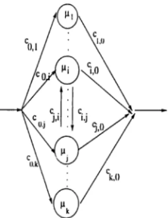
Cox [4] showed that any distribution having a rational Laplace-Stieltjes Transform (LST) can be represented by a set of exponential phases. The LST of any distribution function can be approximated arbitrarily closely by a rational function (Newman and Reddy, [18]). Therefore, in principle, Coxian distributions may represent any distribution either exactly or approximately. The most general form of a distribution that are mixtures of exponential distributions is the family of phase-type distributions. A phase-type distribution with m stages (or phases) is represented in Figure 2.2. The following physical interpretation can be considered: Suppose that an overall task is decomposed into a set of m exponential subtasks. (The processing time of subtask j is exponentially distributed with rate pj.) The first subtask to be processed is j t h one with probability Cq j. Upon completion of subtask j , either subtask к is performed, with probability Cj^k, or the overall task is completed.

with probability cyo- The branching and transition probabilities satisfy, Co,l + ... + Co,m = 1 3,nd Cj-д + ... + = 1

Again the possibility of having a zero processing time with non-zero probability may be added. Note that a Coxian distribution is a special case of phase-type distribution.

Figure 2.2: Phase-type distribution with m phases.

2.1

Definitions and Closure Properties

A phase-type distribution can be considered as the distribution of the time until absorption in an absorbing Markov chain with the states {1,..., m-|-l} with m-|-l being the single absorbing state. Note that since the feasibility and complexity of numerical solutions of Markov processes are very much dependent on the size of the state space, the number of stages of phase-type distributions should be kept as small as possible for modeling purposes. Let Q be the infinitesimal generator of this Markov chain.

Q =

rp po

CHAPTER 2. PHASE-TYPE DISTRIB UTIONS 12

where T is an m x m matrix with Tij > 0 for i^^j and T,·,· < 0 for i= l,...,m . In this representation, m is said to be the order of the phase-type distribution. Then, Te -I- T° = 0, where e is a column vector of ones and the initial probability vector of Q is given by (a, 0!m+i), with a = [ a i ,..., a,„], satisfying oe -f- 0:^+1 = 1. Then T can be considered as the matrix of the rates of transition among the phases and T° is the vector of rates of transition from the transient states

to the absorbing state

D e fin itio n : Let T be a square matrix. The matrix exp(Tx) is given by the following Taylor series expansion:

exp(Tx) = 5:

fc= 0

A

/ + T;r + . . . T'=— -h

for all X 6 R.

L e m m a 2 .2 .2 :(N e u ts , [17], p.45) The distribution function of the time until absorption in the state m-|-l, corresponding to the initial vectorfa, ccm-^-i) is given by,

F(x) = 1 — aexp(Tx)e for x> 0.

L e m m a 2 .2 .1 :(N e u ts , [17], p.45) The states l,...,m are transient if and only if the matrix T is nonsingular.

D e fin itio n :(N e u ts , [17],p.45) A probability distribution F(.) on [0,co) is a distribution of phase-type (PH-distribution) if and only if it is the distribution of the time until absorption in a finite Markov process of the type defined in (1). The pair («,T) is called a representation of F(.).

The phase-type distribution presented in Figure 2.2 can be represented in m atrix notation and any PH-type distribution given in m atrix notation can be represented as shown in Figure 2.2. First we are going to find the m atrix

representation of the PH-type distribution presented in Figure 2.2: It is obvious th at a = [co,i, ...,co,m]· In the T m atrix, T,·,· = —fii for i while Tij =

Cij/ii for i,j = and j. Then the following m atrix of transitions among phases is obtained:

Cl2jUl ClS/J-l

T = C21/U2 - / i2 C23fJ'2 • ^2mf^2

^ml l^m • l^m

W ith the same idea, T°, the vector of rates of transition from the transient states [l,...,m] to the absorbing state is obtained as follows: T° = [cio/Wi, C2o/^2i ···) Crno/im]· Now assume that we have the T matrix of order m, the T° vector, and the initial probability vector a. W hat we aim is to find the transition probabilities Cij shown in Figure 2.2. We can directly equate [cqi, co2, ···) cqtu] = QL- The transition probabilities among the transient phases, Cij — for i,j = l,...,m and iy^ j. The transition probabilities from any transient state to the absorbing state, Cjo = —jl·· This brief discussion shows the ecjuivalence of the graphical and matrix representation of a phase- type distribution. We now present some well-known properties of PH-type distributions:

S o m e p ro p e rtie s :

a. The distribution F(.) has a jump of hight ocm+i at x = 0, and its density function F' (x) on (0,oo) is given by F'{x) = aexp(Tx)T°

b. The Laplace-Stieltjes transform f(s) of F(.) is given by f(s) = OLm+i + a(sI-T)~^T°, for Re s>0

c. The noncentral moments of F(.) are all finite and given by

¡jl\ = (-l)'i!(a T “*e), for i> 0.

CHAPTER 2. PHASE-TYPE DISTRIBUTIONS 14

perform independent multinomial trials with probabilities a i , 0;^, ^m+i, until one of the alternatives occurs. Restarting the process Q in the corresponding state, we consider the time of next absorption and repeat the same procedure there. By continuing this procedure indefinitely a new Markov process is constructed such that (m + 1 )®* state becomes an instantaneous state. This new Markov process with states l,...,m has an infinitesimal generator,

Q* = T +

where T° is an m x m m atrix with identical columns T° and A° = (1 — Q ,„+i)~^diag(ai,..., am)· W ithout loss of generality, we assume that «„,4.1 = 0. The following definition is a characterization PH-type distributions in terms of this modified process:

D e fin itio n :(N e u ts , [17], p.48) The representation (cv,T) is called irreducible if and only if the matrix Q* is irreducible. (From now on, we restrict our attention to irreducible representation.)

2.1.1

Discrete Phase-Type Distributions

Discrete PH-distributions are defined by considering an (m + l)-state Markov chain P of the form,

'jpo

0 1

where I - T is nonsingular. The probability distribution of PH-type is given by:

P =

po = a^+ i Pk = a T '“' ^T° for k > 1.

The corresponding probability generating is the following:

P{z) = am+i

+

and the factorial moments are given by:

2.1.2

Closure Properties

A number of operations on PH-distributions lead again to distributions of PH- type. In each case, a representation for the new distribution is obtained. Before stating the theorems, a notational convention will be presented. If T° is an ?n-vector and (I is an n-vector, the m x n matrix T ° ^ with elements T°/3j, 1 < i < m, 1 < j < n, is denoted by T°B°. The following theorem states that the convolution of two continuous (or discrete) phase-type distributions is also a phase-type distribution.

T h e o re m 2 .2 .2 :(N e u ts, [17], p.51) If F(.) and G(.) are both continuous (or both discrete) PH-distributions with representations (a,T ) and (^,S) of orders m and n respectively, then their convolution F*G(.) is a PH-distribution with representation (7 ,L) given by (in the continuous case):

7 = [«,

L = T T°B°

0 S

T h e o r e m2 .2 .4:(N eu ts, [17], p.53) A finite mixture of PH-distributions is a PH-distribution. If (pi,...,pfc) is the mixing density and Fj{.) has the representation [ a ( i) ,r ( j) ] , 1 < j < k, then the mixture has the representation

QL= \p\QLil),P2QL{2),...,PkQL{k)], and T = T{1) 0 0 T(2) 0 0 0 0 . . T{k)

CHAPTER 2. PHASE-TYPE DISTRIBUTIONS 16

Infinite mixtures of PH-distributions are generally not of phase-type. The following theorem gives an important and useful exception, for which the concept of the K ronecker product of matrices should be introduced.

D e fin itio n :(N e u ts , [17], p.53) If L and M are rectangular matrices of dimension ki x ¿2 and k[ x k'2, their Kronecker product L ^ M is the m atrix

of dimensions k\k[ x ^2^2» written in block-partitioned form as

L \\M L-ioM

LkiiM Lki2M

Lik,M

Lkik2M

Product property: If L, M, U and V are I'ectangular matrices such that the ordinary m atrix products LU and MV are defined, then M) { U (8> =

LU (g) M V

T h e o re m 2 .2 .5 :(N e u ts , [17], p.53) Let {s^} be a discrete PH-density with representation {/dyS) of order n, and F(.) a continuous PH-distribution with representation (a, T) of order m , then the mixture J2'^oSy.F''{.), of the successive convolutions of F(.), is of phase type with representations (7 , L) of order mn, given by

7 = oc(S>§{I —

L = T (g) / -b (1 - am+i) T°A° 0 (7 - + S)~^S 7nzn4-l — Pn+1 “b ^m-fl‘5') S

The following theorem gives the corresponding result of the theorem2.2.5 when F(.) is a discrete PH-distribution.

T h e o r e m2 .2 .6:(N eu ts, [17], p.56) Let {¿t,} and {pt} be discrete PH- densities with representations of {§_,S) and {a,T) of orders n and m respectively. is of phase t}'^pe with representation (x,L ) of order mn, given by,

7 = a ® § ( I - α„г+l‘5')"^

I = T 0 / + (1 - am+i)T°A° <g)(J - + S)~^S

If X and Y are independent random variables with PH-distributions F(.) and G(.), then the distributions Fi(.) =F(.)G (.) and F2(.)= 1 - [1 - F(.)][l - G(.)j, corresponding to max(X,Y) and min (X,Y), are also of phase type. The following theorem provides their phase-type representations:

T lie o re m 2 .2 .9 :(N e u ts, [17], p.60): Let F(.) and G(.) have representations (a, T) and {§jS) of orders m and n respectively, then Fi(.) has the representation (7 , L) of order mn + m + n, given by 7 = [a (g) /5„+ia, am+ i^

L =

T (g )/ + /(8 )5 I ® S ° T ° ^ I

0 T O

0 0 5

and F2(.) has the representation T(g) / + 7(g)5]

2.2

Special PH-Type Distributions

2.2.1

Mixtures of Generalized Erlang (Coxian) Distri­

butions (M G E )

C H A P T E R 2. P H A S E -T Y P E D ISTR IB UTIONS 18

Figure 2.3: Graphical representation of MGE distribution

Holding time in each phase is exponentially distributed with a rate /j,i in phase i. Here, Oj- is the conditional probability that the process visits phase

i + 1 given th at phase i is completed. This probability Co is usually taken to

be 1 . MGE distribution has the following (a, T) representation:

-f.il fiiai -fl2 ft2a2 —fiZ fl3<^3 T = flk-lttk-l -¡J'k , a = (1 , 0, . . ., 0)

T° = [fii{l - ai),fi2{l - d2),...,fik]'^. For k=2, when fii /¿2,

fx{x ) = CiUiC + C2^ 2e x > 0

where Ci = [fii(l — Oi) - — fi2],o.'ndc2 = 1 — ci (See Appendix A for calculations.)

A well-known special case of MGE is the Erlang-distribution with the following graphical representation, for which the density corresponds to that of a Gamma density with parameters k and fi.

Figure 2.4: Graphical representation of the Erlang distribution

2.2.2 Hyper exponential Distribution

A hyperexponential random variable is a proper mixture of exponential random variables with graphical representation shown in Figure 2.5.

Figure 2.5: Graphical representation of the hyperexponential distribution

The exponential random variable with rate fXi is selected with probability Pii 1 ^ For a; > 0, its density function is given by the following function, where the details can be found in the Appendix A:

i=l

Notice that the MGE distribution shown in Figure 2.3 can represent the hyperexponential distribution by taking aj = 0 for all i and a = [pi, ...,pi·].

C H A P T E R 2. P H A S E -T Y P E D ISTR IBU TIO N S 20

2.3

Equivalence Relations Between Some

Classes of PH-Type Distributions

Definition: Two distributions are said to be equivalent if the LST of their density functions are identical.

2.3.1

Exponential and Arbitrary Phase-type Distribu­

tions

Proposition: (Altiok, [1]) A k-phase phase-type distribution is equivalent to an exponential (obviously a single-phase type distribution) distribution with mean

, - i _{provided that the transition rate from every phase to phase k-|-l (absorbing}

phase) is 7 . No restriction is imposed on the structure of the phase-type distribution.

Corollary 1 :(Altiok, [1]) A k-phase MGE distribution is equivalent to an exponential distribution with a mean 7 “^ provided that the rate into state

k -t- 1 from any state is 7 .

IS

Corollary2:(Altiok, [1]) In a trivial case, a hyperexponential distribution i equivalent to an exponential distribution with a mean 7 ” ^, if all the phases have the same mean 7 “^.

2.3.2

Hyperexponential and M G E Distributions

An MGE equivalent will be found of a given k-phase hyperexponential random variable using the transform techniques. We assume that both hyperexponential and the MGE distributions have the same number (k)

of phases. First we are going to find an MGE equivalent to a given hyperexponential distribution. For the MGE distribution, //,· is the rate of the exponential phase and aj gives the conditional probability that the process visits phase i + 1 given that phase i is completed, i= l,...,k . For the hyperexponential distribution, exponential random variable having a rate

Xi is chosen with probability p,·, 1 < i < k. In order to achieve a better insight, before stating the conditions when the equivalent MGE can be found for the given hyperexponential random variable, a m athematical procedure will be shown.

Let the LST of hyperexponential density function be.

H'-is) = Nkis) Dh{s) where Nh{s) = E \ .p¡ n (» + -'>) 1=1 cUld Dfi{s) — n(«5 + A¿) ¿=1 Let the LST of the MGE density function be.

C*{s) = Ncjs) Dc{s) where k ¿“ 1 k ^ c { s ) = - ai)fXi n aif^i I ] (^ + P j ) 1=1 1=1 j=i+l and 0 k ]][ aim = 1 ) n (5 + Pj) = 1 , Oit = 0 1=1 j=k+l and Dc{s) — + f^i) 1=1

C H A P T E R 2. P H A S E -T Y P E D ISTR IB UTIONS 0-2

Our assumption which forces both distributions to have the same number of phases enable us to equate the polynomials. As stated previously, in order that two distributions are equivalent, their LST’s must be equal. One way to achieve this is to equate denominators and numerators by matching the coefficients of the corresponding terms. The fact that there is a one-to-one correspondence in Dh(s) and Dc{s) in terms involving s" ,n = 0,...,^' necessitates fii — Xi. So the denominators of the two LST’s become the same. Now the a,s in the MGE distribution need to be identified. This can be done by equating the coefficients of the corresponding terms in the numerators of the two LSTs. Let,

A;—1 Nh{s) = Y ^ a J 1=0 and N,(s) = Y,c'i.3‘ 1=0

Then, a,s will be found by solving the set of A: — 1 nonlinear equations; Cl = Cl

Cfc-l — Ck-1 (2)

For a given k-phase hyperexponential distribution with Ai > A2 > ... > A^,, there always exists a unique equivalent MGE distributions with m = A,·, for which a,·, ioT i < k will be found solving the A: — 1 nonlinear equations. Now suppose a k-phase MGE distribution with fj, = and a = ( a i ,..., Ck-i) is given and a hyperexponential equivalent is sought (with Xi = fXi for all i). The Pi’s will be found from (2) coupled with the equation J2i=i P t= 1· This can happen only if the ¿1 (squared coefficient of variation) of the MGE distribution is greater than or equal to 1 because cl of hyperexponential is always greater than 1.0. This equivalent hyperexponential is unique.

2.4

Moment Approximations

In this section, the issue of fitting MGE distributions using the method of moments will be summarized. Since the LST of any distribution function can be approximated arbitrarily closely by a rational function, in principle, phase-type distributions may be used to approximate any general distribution. (For convenience, c will denote cl from now on.) It is known that under certain regularity conditions, two distributions coincide if and only if all of their moments coincide. Therefore, in a phase-type approximation, it is desirable to equate as many moments of the phase-type distribution as possible with those of a given general distribution. However, including large number of moments makes the process of characterizing the approximation of phase-type distribution difficult. Therefore usually the first three moments are used for approximation purposes. But it must be noted that the use of the third moment may not always result in an improvement over the use of two moments.

2.4.1

Three-moment approximations

(c > 1)

Altiok [2] suggested a three-moment approximate representation of general distributions. For practical purposes, distributions are distinguished by dividing the range of the squared coefficient of variation into two: c < 1 and c >1. According to the existing empirical results, it does not seem necessary to include the third moment if c < 1 . Therefore, the main concern will be the general distributions with c > 1 , and a set of expressions for their two- phase approximation MGE representations will be developed. The LST of the probability density function of a two stage MGE distribution (with oq = 1 and a is used in place of a-i) is given by;

s/ii(l - a)

L-{s) =

+ H2)+

The first three moments can be found by taking successive derivatives of T*(s), where the set of moments of the original distribution that will be

CH A P TE R 2. PHASE-TYPE DISTRIBUTIONS 24

approximated is denoted by (mi, m2, m3) and the three unknown parameters of the two-stage MGE distribution that will be identified are (yui,/Z2,a).

1 a mi = --- 1---fll fJ'2 which implies a = - 1) Ail m2 = 2(1 - a) [2aniH2 ~ 2a(jUi + /¿2)'^] Ail /il/i2

m3 6(1 - a) [1 2aiJ.i/j,2ipi + /^2) - 6a(^i -|- /¿2)^]

Ai? AiiAii

(3)

(4) (5) (6) Substituting the unknowns (/Ui,/U2,a) into known moments (m i,m2,m 2) from the original distribution, we obtain

X Y

2?ni(/¡7 + 1 ^2) - ”i 2 A i ^ = 2 and 6mi(;tii -(-¿«2)^ - 6mi(/i 1^ 2) - 6(^11 +/«2) - m3Ai?Ai2 = 0

Rewriting the equations in terms of X and Y results in r = (6mi — 3m2/mi) [(6m^/4mi) - m3]

x = ^ + ^

(

)

The positive root is taken as fxi so that fii > 1x2 will hold for c > 1. For the resulting two-stage MGE distribution to be legitimate, ^1 and /22 must be positive and real, and a must be between 0 and 1. For /j.i and fi2 to be positive and real, Y and X should satisfy Y > 0 and X~^ > 4F. If Y is positive, X is always positive, since m i,m2, m 3 are positive numbers and the following condition must hold:

The squared coefficient of variation c is c = {m2/ m l ) — 1 , which implies

m z l m \ > | ( c + 1)^ (12)

Now let us analyze the second necessary condition, namely X~ > A Y . From (8), we have: 1 m.AY m^Y^ (13) 2 _ 1 ru2Y m lY ^ A — —T i---h m l m l 4ml

In order that this expression is greater or equal to 4Y the following inequality should hold,

1 m i ( c + l ) F2

i ( n = - T +_{ml 4} - (3 - c)Y > 0, where g(Y) is convex in Y and its minimum is attained at

(6 - 2c) m f(c + 1 )'^ By inserting (15) into (14) we derive

(14)

(15)

[ ( c + l ) ^ - ( 3 - c ) ^ ]

m l { c + 1)2 > 0 (16)

For (16) to hold we arrive at the condition that c >1 . So, we have shown that

fix and fj,2 are real and fix > fi2 > 0.

Now we are going to analyze possible values of a. Using (3) and (5), we can write 9 1

r)

(17)

For nx > [J.2 the following inequality is obtained

1 - D a >

C H A P T E R 2. P H A S E -T Y P E D ISTR IB UTIONS 26

In order that (19) should hold, a > 0 must be satisfied which is also a necessary and sufficient condition for fXi > H2- From (9) and (10) we know that > ¡j.2·

Hence a > 0 i n ( 1 7 ) and ii\ is always positive if

a <

I P D (20)

Since a > 0, is always greater than 1.0 and therefore a <1 . Clearly, (20) is a tighter bound than 1.0. As D is always greater than 1 , (19) gives a negative lower bound, therefore practically the lower bound for a is zero. Hence, we reach the conclusion that the resulting unique two-stage phase-type distribution is legitimate.

The discussion presented above states that (12) is necessary and sufficient to approximate a distribution with known first three moments and with c > 1.0. If (12) is not satisfied either a three-moment approximation is used at the e.xpense of adding more phases in the MGE distribution or one can choose the nearest acceptable third moment to the original moment or a two-moment approximation can be resorted.

2.4.2

Two moment approximation

The case with c > 1

If first two moments are available, the two-phase MGE distribution can always be found (Marie, [13]). Given that the mean is m\ and the squared coefficient

2 Ail = —_mi

c

Ai2 — —_mi

a = 0.5c

For a two-moment approximation, a hyperexponential distribution with two- phases and a weighted mixing distribution for the branching probabilities in

terms of phase rates ni and is also possible to be found as shown in Figure 2.6. In this case, the equations

+ /^1 — —

mi

2

fJ'llJ'2 = —

m2 have always a solution for c > 1

Il2

Figure 2.6: Weighted Hyperexponential distribution The case with c < 1

For the case c < 1 Erlang distribution is proposed and used as an approximation. (See eg. Sauer and Chandy, [26], Gürler and Parlar, [9] ). The number of stages, k, should satisfy 1 / A : < c < l / A : - 1 . Once k is determined, a Generalized Erlang distribution with a and ^ can be found by.

1 — a = H = 2Â;c + ^ - 2 - + 4 - 4c 2( c + l ) ( i - l ) [1 + (/u — l)a] mi

Chapter 3

The Model and Notations

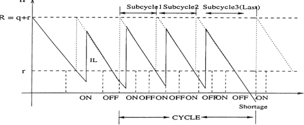
In this chapter, we consider a continuous-review stochastic inventory problem with constant demand and random lead times where the supply is subject to random disruptions. It is assumed that the disruptions of the supplier follow an O N /O FF sequence. When the supplier is ON, the (g,r) policy of Hadley and Whitin [10] is used, i.e., when IP hits the reorder point r, q units are ordered and the target value R = q + r is reached. Here IP is the amount on hand plus on order minus back orders. When the supplier becomes unavailable (OFF), the policy changes so that one orders enough to bring IP to the target level R as soon as the supplier becomes available again. As a consequence, the order c^uantity becomes a random variable in the model.

The supplier O N /O FF status is modeled as a semi-Markov process and the regenerative cycles are defined in the following way: Every tim e the IP reaches

R = r + q right after the completion of an OFF period, the regenerative cycle

starts. We split the regenerative cycles to a random number of sub-cycles which start when the IP is raised to R during the ON period of the supplier. Let N(q) be the number of such sub-cycles which are identical except the last one.

This model is similar to that of Parlar [19] where he assumes that ON periods follow Erlang distribution and OFF periods are general. As an extension of his work, we assume in this study that the ON period is distributed

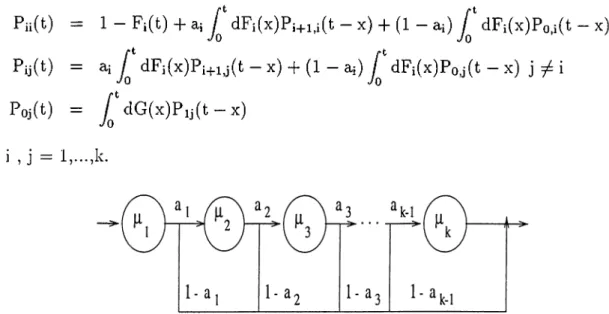
Figure 3.1: Regenerative Cycles of the Inventory Position

with k-stage phase-type distribution (Figure 3.2). This extension is motivated by the approximating properties of Phase-type distributions as reviewed in Chapter 2. The situation can be interpreted as follows; When the period is ON and inventory drops to r, it can be at any stage j , j = Time to stay in stage j is exponentially distributed with rate /ij. Here co,j is the probability th at stage will be the initial stage of an ON period after an OFF period. Upon departure from stage j, either the ON period continues with stage i with probability cj,i or the ON period finishes and an OFF period starts with probability Cj,o· The branching probabilities satisfy,

co,i + ··· + Co,к = 1 3,nd Cj,i + ... -f Cj,k -b Cj,o = 1

The OFF period which is assumed to follow a general distribution is denoted by 0 .

C H A P T E R 3. T H E M ODEL AND NOTATIONS ₃₀

Figure 3.2: Phase-type distribution with k phases.

3.1

The Semi-Markov Processes and The

Objective Function

Let {C(t)> t > 0} be the semi-Markov process representing ON /O FF status of the supplier such that ^(t) = 0 corresponds to the OFF period and C(t) = j indicates that the supplier is at the stage of the ON period. Note that the duration of stay in any state j , j = is exponential. We define Pij(t) = P{(^(t) = j I C(0) = i }, i,j = l,2,...,k,0 as the transition functions of the SMP. Our aim now is to find the {q, r) values which minimize the long run average cost function. The representation in terms of a semi-Markov process allows us to use the renewal reward theorem (Ross, [25]) which states that the long run average cost function is the ratio of the expected cycle cost to expected cycle length. We first consider below the cycle length.

3.1.1

Cycle Length

The Theorem of Parlar [19] below is useful in our case to find the expected value of the cycle length therefore we present it together with its proof for the sake of completeness. Let T, be the time required to complete the cycle if the process is at state i, i = l,...,k , and Ti denote the expectation of Ti and To be the ’waiting tim e’ for the supplier to return to the ON state. For any vector

V, let denote its transpose. We denote the constant demand rate with D.

T h e o re m 1 . (P a rla r, [19]) The Tj, i = I v 'k ? values are obtained from the solution of the linear system,

( I - P ) T = b

where I is the identity matrix, and

P = [Pij(q/D)j, i,j = l,...,k ,

= [Ti,...,Tk],

b ^ = [ q / D + T o P i o ( q / D ) , . . . , q / D + T o P k o ( q / D ) j .

(1)

P ro o f. Conditioning on the state found when the inventory reaches r after

q / D time units and using the renewal argument, we obtain, for i = l,...,k i q / D + T i i f C ( q / D ) = i

t i = |q/D + Tj ifC(q/D) =j , j = j i (2) [ q/D + to if C(q/D) = 0

Taking expectations in 2, we have

T i = ¿ [ q / D + T j ] P i i ( q / D ) + [ q / D + T o ] P i o ( q / D ) , i = 1 ... k ( 3 )

j=l

Collecting terms containing the unknowns on the left-hand side gives for i= l,...,k ,

T i ( l - P i i ( q / D ) ) - ^ T j P i j ( q / D ) = q / D + T o P i o ( q / D ) , ( 4 )

Writing 4 using matrix notation, we obtain (I - P ) T = b. □

R e m a r k s . 1. The results can easily be modified for the case when the demand is random. In particular equation 4 would be replaced by,

C H A P T E R 3. T H E M ODEL AND NOTATIONS 32

and the rest of the modification would be obvious. However to keep the presentation simple we take the demand as constant.

R e m a r k s .2 . Note that in Parlar’s model, every time a regenerative cycle starts, the process is in the first stage of the ON period. But in our case the first stage the cycle starts is random. We therefore need the following proposition.

P r o p o s itio n ! . Expected cycle length T(q) is,

T(q) = [co,i,....,Co.k](I-P)-^b

P ro o f. When Figure 3.2 is examined it is seen that a cycle may start with any stage i, i = l,...,k with probability co,j. Therefore the cycle length T(q) is found by summing the products of the initial state probabilities with the corresponding expected cycle lengths. □

3.1.2

Cycle Cost

A complete cycle consists of a random number of sub-cycles of length q/D and a final one of a longer length due to the ’waiting’ time until the supplier becomes ON again.

Let K be the ordering cost per order, h be the holding cost per unit per unit time and b be the backorder cost per unit which are same for all sub-cycles. Other than the ordering cost, the expected inventory (or average inventory) carrying cost should be calculated. By definition, the net inventory is the on hand inventory minus the backorders. Then the expected on hand inventory is equal to the expected net inventory plus the expected number of backorders. The cost incurred in the shorter sub-cycles is the cost of a cycle in the standard H adley/W hitin {q,r) model, (i.e., a ’standard cycle’). While computing the inventory holding cost, we will use the assumption made by Hadley and Whitin that the expected number of backorders is negligible.

Let c(q,r) be the cost of an arbitrary sub-cycle before the last one with c(q,r)=E[c(q,r)]. Besides the ordering cost, the other components of this cost are as follows:

i)Holding Cost:

Let L be the (possibly random) lead-time with a p.d.f of gL(0 Z be the demand during L. By definition, safety stock Sz is the expected value of the inventory level (IL, which is inventory on hand minus the backorders) just before an order arrives, i.e, Sz = E[IL(Z, r)]

where IL(Z,r) = r - Z = r - LD. Then

roo

Sz = E[IL(Z, r)] = / (r - z)kz(z)dz = r — 4>

J o

where

kz(z) = ^ g U z / D ) (5)

and <j) = zkjdz = E[Z] is the expected demand during L. The expected net inventory immediately after the delivery of the ordered q units is q -|- Sz· Then at the start of these cycles, the net inventory will be q -b Sz and at the end of the cycle it will be just Sz- These will be also the expected values of the on hand inventory as we assume that the expected number of back orders can be neglected. We derive that the average inventory during a cycle is

9<1 + Sz

In order to find the total expected inventory during a cycle, we should multiply the average inventory with the cycle length q/D , which gives

1 Then, ^qVD -b Szq/D. .1 E[holding cost] = h[-q^/D -b (r — (^)q/Dj L· (6)

C H A P T E R 3. T H E M ODEL AND NOTATIONS 34

Actual number oi back orders ?7L(Z,r) during a standard cycle depends on the reorder point r and the demand Z during the lead time L. That is,

/;l(z, r) = I(z > r)(z - r) where I(z > r) is the indicator function. Then, letting ^L(r) = /,.°°(z — r)kz(z)dz be the expected number of back orders during a standard cycle, we have

E[back order cost] = b/7L(r) ₍₇₎

Combining all the individual expected costs, i.e., ordering cost K, (6) and (7) will give us the expected cost per standard cycle as,

c(q, r) = K + h [iq V D + (r - <A)q/D] + b^L(r)

We now consider the cost of the last sub-cycle. Suppose C(q,r) is the cost of the last sub-cycle in the model and let C(q,r) = E[C(q,r)j. Besides the ordering cost, the other components of this cost are as follows:

iii) Holding cost:

Let ?/^ = To -|- L be the length of the total delay, i.e., the lead time and the ’waiting’ time for the supplier to return to the ON state after an order attem pt is made. Also let W be the demand during Tq. Then U = W -f- Z be the combined demand during V*· Then the safety stock Su is the expected value of the inventory level (IL) just before the order arrives when the supplier returns to the ON state, i.e., Su = E[IL(U,r)j = r - U.

If g>(T) is the p.d.f of the total delay random variable V’, then

where

roo

Su = / (r - u)ku(u)du = r - (f,

Jo

ku(u) = ^gv-(u/D) ₍₈₎

is the marginal density of the demand during the total delay V’ and ( = uku(u)du = E[U] is the expected demand during the total delay. It must be noted that in the last sub-cycle the order quantity is a random variable since